Data reduction for the AMBER instrument

(1)

HAL Id: hal-00008536

https://hal.archives-ouvertes.fr/hal-00008536

Submitted on 7 Sep 2005

HAL is a multi-disciplinary open access

archive for the deposit and dissemination of

sci-entific research documents, whether they are

pub-lished or not. The documents may come from

teaching and research institutions in France or

abroad, or from public or private research centers.

L’archive ouverte pluridisciplinaire HAL, est

destinée au dépôt et à la diffusion de documents

scientifiques de niveau recherche, publiés ou non,

émanant des établissements d’enseignement et de

recherche français ou étrangers, des laboratoires

publics ou privés.

Data reduction for the AMBER instrument

Florentin Millour, E. Tatulli, A. Chelli, G. Duvert, G. Zins, B. Acke, F.

Malbet

To cite this version:

Florentin Millour, E. Tatulli, A. Chelli, G. Duvert, G. Zins, et al.. Data reduction for the AMBER

instrument. New Frontiers in Stellar Interferometry, 2004, France. pp.1222. �hal-00008536�

(2)

ccsd-00008536, version 1 - 7 Sep 2005

Data reduction for the AMBER instrument

F. Millour

a

, E.Tatulli

a

, A. Chelli

a

, G. Duvert

a

, G. Zins

a

, B. Acke

a

and F. Malbet

a a

LAOG, Observatoire de Grenoble, BP 53, F-38041 Grenoble CEDEX 9, FRANCE;

ABSTRACT

We present here the general formalism and data processing steps used in the data reduction pipeline of the AMBER instrument. AMBER is a three-telescope interferometric beam combiner in J, H and K bands installed at ESO’s Very Large Telescope Interferometer. The fringes obtained on the 3 pairs of telescopes are spatially coded and spectrally dispersed. These are monitored on a 512x512 infrared camera at frame rates up to 100 frames per second, and this paper presents the algorithm used to retrieve the complex coherent visibility of the science target and the subsequent squared visibility, differential phase and phase closure on the 3 bases and in the 3 spectral bands available in AMBER.

Keywords: AMBER, VLTI, Long Baseline Infrared Interferometry, Complex Visibility, P2VM Algorithm, Data Reduction Software, Spectroscopy, Spatial Coding, Phase Closure, Interspectrum

1. INTRODUCTION

AMBER1_{makes fringes on an infrared detector. Before combination, a spatial filtering}2_{is made by optics fibers}

in order to keep only the central part of the airy disk of the telescope. These fringes are spatially coded, i.e. their spatial frequency is fixed by the instrument setup, and the spatial frequency of fringes due to a pair of telescopes is different from the spatial frequency of another pair. In the following we will treat the case of only one pair of telescopes. The case of 3 telescopes can easily be deduced from the equations given in this article.

The equations are given for one wavelength, so every value in this article should be interpreted as wavelength dependant. The interferometric equation describes the interferometric signal pixel per pixel:

ik= N p1a1k+ N p2a2k+ 2N V√p1p2√a1ka2kcos(2πf αk+ φak+ φp+ φo) (1)

In this equation k is the pixel index, ik is the number of photo-events in pixel k of the interferometric channel,

N is the unknown object’s flux, p1and p2are transmission coefficients for the two combined beams, and a1kand

a2k are related to specific features of each pixel. V is the amplitude of the complex visibility.

Furthermore, 4 phases are to be taken into account: f corresponds to the combining baseline b (f = b/λ), αk

is an angle that indicates the position of each pixel, φak is a phase factor that accounts for optical aberrations

in the instrument (which are expected to be negligable) and φois the object’s phase. When measuring a source

through the turbulent atmosphere, another phase factor enters the equation: the differential piston φp. While

measuring this interferogram, the photometric variability in both input beams is recorded simultaneously in the

photometric channels. Let’s call P1 and P2 the measured flux in photometric channels 1 and 2 respectively.

Hence one can define the coefficients v1k and v2k as

P1v1k = N p1a1k (2)

P2v2k = N p2a2k (3)

If one can determine the vk values, one can compute the continuum corrected interferogram mk defined by

mk = ik− P1v1k− P2v2k = 2N V√p1p2√a1ka2kcos(2πf αk+ φak+ φp+ φo) (4)

Notice that there are 3 sets of vk when one works with 3 input beams.

Further author information: (Send correspondence to F.M.)

(3)

In the case of AMBER data reduction, we decided not to use the “traditional” Fourier transform algorithm3

because of the precision required in the specifications of the instrument (1% for the fringe contrast). For that purpose we developped an algorithm that generalizes to more than 4 pixels the well known ABCD algorithm

and which is called “P2VM”4 _{as for Pixel-To-Visibility-Matrix algorithm.}5 _{It takes into account the shape of}

the output beam of the instrument6in order to accurately calibrate the intrumental factor in the visibilities and

can be interpreted in the Fourier space as a Fourier transform where the shape of the fringe peak is fitted.

2. THE DATA REDUCTION SOFTWARE

2.1. Overview

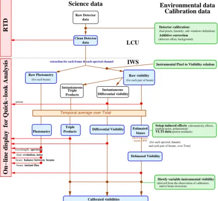
For the implementation in the Data Reduction Software, we wrote a c library called amdlib (stands for AMber Dcs LIBrary) that handles the raw data, the calibration data and computes the P2VM and the subsequent

visibilities7 _{(figure 1). We decided to use the same library for quickLook on the AMBER workstation to help}

the astronomer to evaluate in real time the quality of the data, and for offline data reduction.

0 0 1 1 00 00 11 11 0 0 1 1 0 0 1 1 0 0 1 1 0 0 1 1 00 00 11 11 0 0 1 1 0 0 0 1 1 1 0 0 0 1 1 1 0 0 0 1 1 1 0 0 1 1 0 0 1 1 Triple Products Instantaneous

and each pair of beams, over Tstat) (for each spectral channel,

Raw Detector data

Instantaneous Differential visibility

Science data

and/or beam inversion) (derived from the observation of calibrators photon noise, mean OPD Environmental data Calibration data 0 0 1 1 LCU IWS RTD

(detector offset, background)

Instrumental Pixel to Visibility relation Detector calibration: Additive correction

Triple

Products Differential Visibility Estimated _biases

Setup induced effects (chromaticity effects, readout noise, polarisation)

VLTI data (piston residuals)

Slowly variable instrumental visibility

wavelength: spectrum time: evolution, noise beam: balance between

beam: instant flux

Debiassed Visibility

(bad pixels, linearity, sub−windows definition)

beams

Calibrated visibilities Clean Detector

data

Raw Photometry

(for each beam)

Raw visibility

(for each pair of beam)

Temporal average over Tstat

On−line display for Quick−look Analysis

extraction for each frame & each spectral channel

Photometry

piston

Figure 1.AMBER Data Reduction Roadmap

This library can be linked with a data reduction software like IDL, SciLab, etc. We developped at LAOGa

the complete linking with the open source IDL-like software of John Munro called Yorick

(ftp://ftp-icf.llnl.gov/pub/Yorick/doc/index.html). The following figures illustrating this paper have been

pre-pared with Yorick using amdlib on real fringes obtained on Sirius in March 2004 with VLTI-AMBER.8

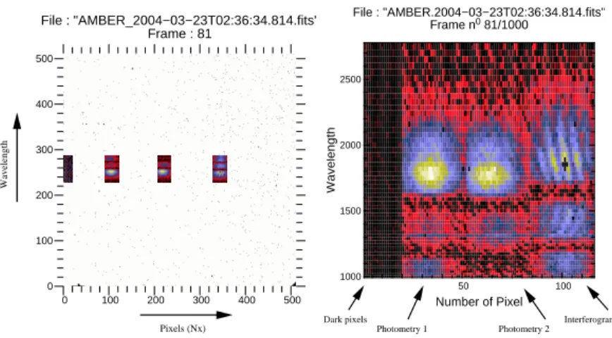
The detector of AMBER takes only a part of the total detector array for rapid frames observing needs, as shown in figure 2. This is why the AMBER images seem to have sometimes “steep edges”, when the detector windows are not well centered on the actual beam.

(4)

0 100 200 300 400 500 0 100 200 300 400 500 File : "AMBER_2004−03−23T02:36:34.814.fits" Frame : 81 Wavelength Pixels (Nx) 50 100 1000 1500 2000 2500 File : "AMBER.2004−03−23T02:36:34.814.fits" Frame n0_81/1000 Number of Pixel Wavelength

Photometry 1 Photometry 2 Interferogram Dark pixels

Figure 2.Placement of the data window in the detector array and a corresponding displayed frame in the data reduction

software. Note that the wavelength table is not correct but it will be updated in the later steps of the data reduction.

2.2. P2VM Computation Preparation

For an accurate estimation of the complex visibilities of the scientific object, one needs to completely calibrate the behaviour of the instrument, which leads to accurately characterize the spatial frequency of the fringes and the shape of the output beams. The P2VM calibration is aimed at reaching this goal with some constraints as, for example, a very hard stability requirement of the instrument.

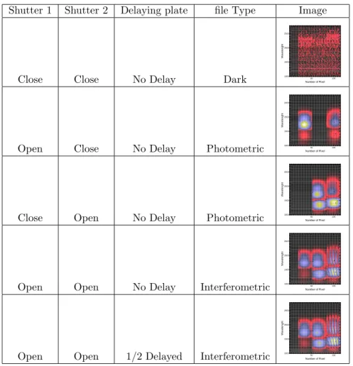
A P2VM “calibration” is performed by obtaining one frame with all shutters closed to get a ’sky-type’ frame, then by opening in turn only one shutter to get the shape of the illumination in the interferometric channel due

to one fiber (the so-called vi

k), then by opening in turn pairs of shutters to retrieve the interference fringe pattern

for each pair of telescope, with and wihout a phase shift of a known value γ0(figure 3).

The visibility of the artificial source (lamp) in the Calibration and Alignment Unit (CAU) of AMBER is

supposed to be fixed, calibrated and noted Vc.

Those calibration frames are processed with amdlib routines to produce a P2VM used for all following visibility extractions, until the Instrument Setup changes and a new P2VM is needed.

2.3. P2VM Computation

The first of the previously described calibration frames is a sky-like measurement, without input light. This is done in order to substract the uncorrelated light ’sky’ due to the thermal emission of the fibers, if any. The frames

number 2 and 3 are exposures with only one input beam (figure 4). This allows one to compute the vk coefficients

in the equations described before, by dividing the interferometric channel by the measured photometric flux, pixel per pixel and for every input beam.

The other 2 frames completely determine the calibration of the instrument. In these frames, two input beams at a time are combined. Two exposures are made per baseline. In one of this couple of frames, an additional phase shift is inserted into one of the beams. This results in an extra phase factor in the interferometric equation,

which is called γ0. Hence one has the following equations:

i0

k = N0p1a1k+ N0p2a2k+ 2N0Vc√p1p2√a1ka2kcos(2πf αk+ φak+ φc) (5)

for the frame without an additional phase shift (indicated as0_{) and}

iγ0

k = Nγ

0_p

1a1k+ Nγ0p2a2k+ 2Nγ0Vc√p1p2√a1ka2kcos(2πf αk+ φak+ φc+ γ0) (6)

for the frame with an extra phase shift (indicated as γ0_{). V}

c and φc are respectively the known visibility and

phase of the calibration source. The continuum corrected interferograms for both frames are

m0_k= 2N0Vc√p1p2√a1ka2kcos(2πf αk+ φak+ φc) (7)

mγ0

k = 2N γ0

(5)

Shutter 1 Shutter 2 Delaying plate file Type Image

Close Close No Delay Dark 1000 50 100

1500 2000 2500

Number of Pixel

Wavelenght

Open Close No Delay Photometric 1000 50 100

1500 2000 2500

Number of Pixel

Wavelenght

Close Open No Delay Photometric 1000 50 100

1500 2000 2500

Number of Pixel

Wavelenght

Open Open No Delay Interferometric 1000 50 100

1500 2000 2500

Number of Pixel

Wavelenght

Open Open 1/2 Delayed Interferometric 1000 50 100

1500 2000 2500

Number of Pixel

Wavelenght

Figure 3.Complete calibration sequence for 2 telescopes taken with the internal calibration source (CAU)

2.0 2.5 0.0 0.5 1.0 1.5 10+6 2.0 2.5 0.0 0.5 1.0 1.5 10+6 Photometry I1 Wavelenght (µm) I2

(6)

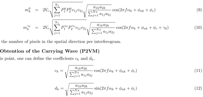
Knowing of P0

1v1k, P20v2k, P1γ0v1k and P2γ0v2kand the relations 2 and 3 are used to eliminate the unknown fluxes

N0 _{and N}γ0 _{from equations 7 and 8. One obtains}

m0_k = 2Vc v u u t Nx X j=1 P0 1P20v1jv2j s a1ka2k PN x j=1a1ja2j cos(2πf αk+ φak+ φc) (9) mγ0 k = 2Vc v u u t Nx X j=1 Pγ0 1 P γ0 2 v1jv2j s a1ka2k PN x j=1a1ja2j cos(2πf αk+ φak+ φc+ γ0) (10)

Nxis the number of pixels in the spatial direction per interferogram.

2.4. Obtention of the Carrying Wave (P2VM)

At this point, one can define the coefficients ck and dk,

ck = s a1ka2k PN x j=1a1ja2j cos(2πf αk+ φak+ φc) (11) dk = s a1ka2k PN x j=1a1ja2j sin(2πf αk+ φak+ φc) (12)

called the real and imaginary part of the carrying wave of the interferometer (for this wavelength and for this baseline). Making use of this notation, one can write the continuum corrected interferograms as:

m0_k = 2Vc v u u t Nx X j=1 P0 1P20v1jv2j× ck (13) mγ0 k = 2Vc v u u t Nx X j=1 Pγ0 1 P γ0 2 v1jv2j× (ckcos γ0− dksin γ0) (14)

In these equations, ck and dk are the only unknown values, so they can be computed.

2.0 2.5 10 20 30 2.0 2.5 10 20 30 Ck Nx Dk Wavelenght (µm) Nx 10 20 30 −0.1 0.0 0.1 0.2 10 20 30 −0.2 −0.1 0.0 0.1 Ck at 2.41 µm Ck Dk at 2.41 µm N0_{of pixel} Dk 2.0 2.5 −100 −50 0 50 100 2.0 2.5 0.0 0.2 0.4 0.6 0.8 Instrumental Contrast. V MCS Phase Wavelenght (µm) φ

Figure 5.The carrying waves obtained in the P2VM in the 2 telescopes case (left & middle), the corresponding

instru-mental contrast (top right) and the phase γ0 that can be recalibrated from the P2VM data (bottom right)

The real and imaginary parts of the carrying waves for each pixel and for all wavelengths are the inputs of the

pixel-to-visibility matrix P2VM (figure 5). Thus, this matrix has dimensions (Nx× 6) in the case of 3 telescopes

(7)

provided to the second part of the data reduction. One can determine the instrumental contrast by the data contained in the P2VM (figure 5):

V_inst2 = N x X j=1 c2_k+ d2_k (15)

2.5. Visibility extraction

Once a P2VM has been recorded, visibility extraction can be performed on all following observations. Indeed, let us start with the interferometric equation for two telescopes:

ik= N p1a1k+ N p2a2k+ 2N V(12)√p1p2√a1ka2kcos(2πf(12)αk+ φ

(12) ak + φ

(12)

p + φ(12)o ) (16)

One can remark that the spatial coding of the interferogram is captured in the quantity f(12). One can use

the monitored photometric flux P1v1k, P2v2k and the calibrated vik coefficients in each beam to pass from the

interferogram given by equation 16 to the continuum corrected interferogram with the relations 2 and 3. Let us consider the continuum corrected interferogram for the two telescopes case.

mk = 2N V(12)√p1p2√a1ka2kcos(2πf(12)α (12) k + φ (12) ak + φ (12) p + φ(12)o + φ(12)c − φ(12)c ) (17) Defining Φ(12)_{= φ}(12)

p + φ(12)o − φ(12)c for baseline 12 leads to

mk = 2N V(12)√p1p2 v u u t Nx X j=1 a1ja2j(c(12)k cos Φ (12) − d(12)k sin Φ (12)₎ ₍₁₈₎

One can define the weighted complex visibility for baseline 12 as C12= R12+ iI12 where

R12= 2N V(12)√p1p2 v u u t Nx X j=1 a1ja2j× cos Φ(12) (19) and I12= 2N V(12)√p1p2 v u u t Nx X j=1 a1ja2j× sin Φ(12) (20)

are the real and imaginary parts. From equations 18, 19 and 20 the meaning of the name ’carrying waves’ is clear. They are the physical quantities that support the weighted complex visibilities.

The continuum corrected interferogram for two baselines (18) can now be written as:

mk = c(12)_k R12− d(12)_k I12 (21)

The R12and I12 are estimated from the data for every science frame and wavelength by minimising

χ2R,I = Nx X j=1 mj− c (12) j R12+ d(12)j I12 σmj !2 (22) In this formula, σ2

mj is the formal variance of mj (assuming only photon and detector noises):

σm2j = σ 2 ij + 2 X k=1 v2kjσP2k (23)

assuming Poisson statistics

σ_i2_j = i¯j+ σdet2 (24)

σ2Pk = P¯k+ σ

2

(8)

σ2

det is the detector noise (≈ 15e−). For fair enough signal-to-noise rates, σm2j can be defined instantaneously,

with ¯ij= ij and ¯Pk= Pk. The atmospheric influence on this variance is neglected at this point.

Notice that one can write equation 21 as a matrix multiplication, where [mk], P 2V M and [R, I] respectively

have dimensions (Nx× 1), (Nx× 2) and (2 × 1) for each spectral channel.

[mk] = P 2V M × [R, I] (26)

Finding the linear least square fit values for [R, I] is equivalent to ’invert’ P2VM, taking into account the pixel-to-pixel covariance matrix COV .

[R, I] = (tP 2V M × COV−1_{× P 2V M)}−1_× t_{P 2V M × COV}−1_[m

k]

= invP 2V M [mk] (27)

Notice that (t_{P 2V M × COV}−1_{× P 2V M) is a square symmetrical matrix with non-zero diagonal entries, so}

inverting is possible. The covariance matrix is a (Nx× Nx) diagonal matrix with

COV (j, j) = σm2j (28)

for j = 1 . . . Nx. The cross-correlation of two different pixels is neglected here. It is also possible to define

the covariance matrix as an average over a certain number of frames, using equation 23 with averaged values ¯

ij =< ij >f rames and ¯Pk =< Pk >f rames. This avoids numerous inversions (for each frame) during the

calculations of the R and I quantities.

The figure 6 shows the phases (arcTangent of I/R) of the complex visibilities computed in amdlib. The wavelength table was not up to date at the time of the observation but the phases are well aligned in the K band (where there is enough flux).

2.6. From weighted complex visibilities to visibilities

The weighted complex visibilities are the bricks to build the required observables (squared visibility, differential phase, closure phase, etc.). We will present here only the squared visibility estimation.

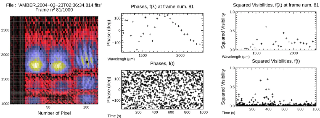
50 100 1000 1500 2000 2500 File : "AMBER.2004−03−23T02:36:34.814.fits" Frame n0_81/1000 Number of Pixel Wavelenght 200 400 600 800 1000 −100 0 100 1500 2000 −100 0 100 Phase (deg) Wavelengh (µm)

Phases, f(λ) at frame num. 81

Phases, f(t) Phase (deg) Time (s) 200 400 600 800 1000 0.0 0.5 1.0 1500 2000 0.0 0.5 1.0 Squared Visibility Wavelength (µm)

Squared Visibilities, f(λ) at frame num. 81

Squared Visibilities, f(t)

Squared Visibility

Time (s)

Figure 6.Example of an observation taken on Sirius during Assembly, Integration and Verification of AMBER9

in March 2004 (fringe pattern at the left). Top middle is the instantaneous visibilities phase on a frame where there was flux in both telescopes. The H band did not have much flux, that is why the phases seems erratic while in the K band there was flux and the phases are well aligned. This was not all the time the case and is why the phase in one spectral channel is uniformely spanned (bottom middle). In the same frame, the instantaneous squared visibilities are quite high (top right) as in one spectral channel they are almost always null as the photometry is low (bottom right) due to the bad injection in the fibers with the testing siderostat of the VLTI.

(9)

The visibility is estimated starting from the squared norm of C12, averaged over a number of frames. Again

we use formulas 2 and 3 to estimate the unknown prand ark values. Inserting these expressions into equations

19 and 20, one obtains with |C12|2− bias(t) = R212+ I122 − bias(t)

V122 =

< R2

12+ I122 − bias(t) >t

4 < P1P2>tPNj=1x v1jv2j

(29)

The unbiasing of the squared weighted visibilities is necessary, as for the Fourier transform algorithm.10 _This

leads to a change on the error on C12 with an expected value of 0 into a squared error with a non-zero mean.

The debiasing is done instantaneously by estimating the photon bias and the detector bias.

The figure 6 shows an instantaneous measurement of the squared visibility on the star Sirius taken during April 2004 at Paranal. The measured precision on the sky is about 1% so the goal of getting accurate visibilities with the P2VM has been achieved in the case of AMBER.

2.7. The differential phase estimator

The unbiased differential phase between λ1 and λ2 is given directly from the averaged interspectrum of the

complex visibility C12by

∆Φλ1λ2= atan < C_12,λ1C

∗

12,λ2 > (30)

2.8. The closure phase estimator

As for the differential phase, the closure phase is given directly from the averaged triple product of the complex

visibilities C12C23and C13, only in the 3 telescopes case by

Φobject123 = atan < C12C23C13∗ > +Φinstrument123 (31)

where Φinstrument

123 has to be calibrated on a point source.

3. CONCLUSION

In this paper we present the AMBER data reduction software based on a generalization of the ABCD method to get visibilities called “Pixel To Visibilities Matrix” algorithm. With this formalism, one can accurately calibrate the instrument configuration and get accurate measurements of the source visibilities, closure phases and differential phases.

One can then use these observables, corrected from the atmosphere transfert function11_{to extract the useful}

(10)

REFERENCES

1. R. G. Petrov, F. Malbet, G. Weigelt, F. Lisi, P. Puget, P. Antonelli, U. Beckmann, S. Lagarde, E. Lecoarer, S. Robbe-Dubois, G. Duvert, S. Gennari, A. Chelli, M. Dugue, K. Rousselet-Perraut, M. Vannier, and D. Mourard, “Using the near infrared VLTI instrument AMBER,” in Interferometry for Optical Astronomy II. Edited by Wesley A. Traub . Proceedings of the SPIE, Volume 4838, pp. 924–933, Feb. 2003.

2. P. Mege, F. Malbet, and A. Chelli, “Spatial filtering in AMBER,” in Proc. SPIE Vol. 4006, p. 299-307, Interferometry in Optical Astronomy, Pierre J. Lena; Andreas Quirrenbach; Eds., pp. 299–307, July 2000. 3. V. Coud´e Du Foresto, S. Ridgway, and J.-M. Mariotti, “Deriving object visibilities from interferograms

obtained with a fiber stellar interferometer,” A&AS 121, pp. 379–392, Feb. 1997. 4. K. H. Hofmann, MEMO AMBER-IGR-013 : Calibrating the visibilities, Dec. 1999.

5. A. Chelli, MEMO AMBER-IGR-018 : Visibility, Differential Phase and Closure Phase Estimators in the Image Space, July 2000.

6. K. H. Hofmann and F. Malbet, MEMO AMBER-OSM-006 : A proposition for the AMBER visibility esti-mator, May 1998.

7. G. Duvert, R. G. Petrov, and P. Antonelli, VLT-PLA-AMB-15830-6004 : AMBER Data Reduction Plan, Oct. 2003.

8. ESO Press Release, “Adding New Colours to Interferometry,” Apr. 2004.

9. S. Robbe-Dubois, R. G. Petrov, U. Beckmann, S. Lagarde, F. Lisi, F. Malbet, P. Antonelli, Y. Bresson, A. Roussel, D. Mourard, A. Delboulbe, G. Duvert, P. Kern, E. LeCoarer, F. Millour, K. Rousselet-Perraut, G. Zins, M. Heininger, G. Weigelt, P. Stefanini, M. Accardo, C. Gil, N. Haddad, N. Housen, M. Kieke-busch, P. Mardones, F. Puech, F. Rantakyro, A. Richichi, M. Schoeller, and M. Vannier, “The VLTI focal instrument Amber : results of the first phase of the Alignment, Integration and Verification in Paranal,” in Astronomical Telescopes and Instrumentation, New frontiers in Stellar Interferometry, Proceedings of the SPIE, Volume 5491: these proceedings, July 2004.

10. G. Perrin, “Subtracting the photon noise bias from single-mode optical interferometer visibilities,” A&A 398, pp. 385–390, Jan. 2003.

11. G. Perrin, “The calibration of interferometric visibilities obtained with single-mode optical interferometers. Computation of error bars and correlations,” A&A 400, pp. 1173–1181, Mar. 2003.