Simulations of preindustrial, present-day, and 2100 conditions in the NASA GISS composition and climate model G-PUCCINI

(1)

HAL Id: hal-00301540

https://hal.archives-ouvertes.fr/hal-00301540

Submitted on 15 Jun 2006

HAL is a multi-disciplinary open access

archive for the deposit and dissemination of sci-entific research documents, whether they are pub-lished or not. The documents may come from teaching and research institutions in France or abroad, or from public or private research centers.

L’archive ouverte pluridisciplinaire HAL, est destinée au dépôt et à la diffusion de documents scientifiques de niveau recherche, publiés ou non, émanant des établissements d’enseignement et de recherche français ou étrangers, des laboratoires publics ou privés.

Simulations of preindustrial, present-day, and 2100

conditions in the NASA GISS composition and climate

model G-PUCCINI

D. T. Shindell, G. Faluvegi, N. Unger, E. Aguilar, G. A. Schmidt, D. M.

Koch, S. E. Bauer, R. L. Miller

To cite this version:

D. T. Shindell, G. Faluvegi, N. Unger, E. Aguilar, G. A. Schmidt, et al.. Simulations of preindustrial, present-day, and 2100 conditions in the NASA GISS composition and climate model G-PUCCINI. Atmospheric Chemistry and Physics Discussions, European Geosciences Union, 2006, 6 (3), pp.4795-4878. �hal-00301540�

(2)

ACPD

6, 4795–4878, 2006 Composition and climate modeling with G-PUCCINI D. T. Shindell et al. Title Page Abstract Introduction Conclusions References Tables Figures J I J I Back Close

Full Screen / Esc

Printer-friendly Version

Interactive Discussion

EGU

Atmos. Chem. Phys. Discuss., 6, 4795–4878, 2006 www.atmos-chem-phys-discuss.net/6/4795/2006/ © Author(s) 2006. This work is licensed

under a Creative Commons License.

Atmospheric Chemistry and Physics Discussions

Simulations of preindustrial, present-day,

and 2100 conditions in the NASA GISS

composition and climate model

G-PUCCINI

D. T. Shindell1,2, G. Faluvegi1,2, N. Unger1,2, E. Aguilar1,2, G. A. Schmidt1,2, D. M. Koch1,3, S. E. Bauer1,2, and R. L. Miller1,4

1

NASA Goddard Institute for Space Studies, New York, NY, USA 2

Center for Climate Systems Research, Columbia University, NY, USA 3

Dept. of Geophysics, Yale University, New Haven, USA 4

Dept. of Applied Physics and Applied Math, Columbia University, NY, USA

Received: 3 February 2006 – Accepted: 13 March 2006 – Published: 15 June 2006 Correspondence to: D. T. Shindell ([email protected])

(3)

ACPD

Full Screen / Esc

EGU

Abstract

A model of atmospheric composition and climate has been developed at the NASA Goddard Institute for Space Studies (GISS) that includes composition seamlessly from the surface to the lower mesosphere. The model is able to capture many features of the observed magnitude, distribution, and seasonal cycle of trace species. The simulation

5

is especially realistic in the troposphere. In the stratosphere, high latitude regions show substantial biases during period when transport governs the distribution as meridional mixing is too rapid in this model version. In other regions, including the extrapolar tropopause region that dominates radiative forcing (RF) by ozone, stratospheric gases are generally well-simulated. The model’s stratosphere-troposphere exchange (STE)

10

agrees well with values inferred from observations for both the global mean flux and the ratio of Northern to Southern Hemisphere downward fluxes.

Simulations of preindustrial (PI) to present-day (PD) changes show tropospheric ozone burden increases of 11% while the stratospheric burden decreases by 18%. The resulting tropopause RF values are −0.06 W/m2 from stratospheric ozone and

15

0.40 W/m2 from tropospheric ozone. Global mean mass-weighted OH decreases by 16% from the PI to the PD. STE of ozone also decreased substantially during this time, by 14%. Comparison of the PD with a simulation using 1979 pre-ozone hole conditions for the stratosphere shows a much larger downward flux of ozone into the troposphere in 1979, resulting in a substantially greater tropospheric ozone burden than that seen in

20

the PD run. This implies that reduced STE due to Antarctic ozone depletion may have offset as much as 2/3 of the tropospheric ozone burden increase from PI to PD. How-ever, the model overestimates the downward flux of ozone at high Southern latitudes, so this estimate is likely an upper limit.

In the future, the tropospheric ozone burden increases sharply in 2100 for the A1B

25

and A2 scenarios, by 41% and 101%, respectively. The primary reason is enhanced STE, which increases by 71% and 124% in the two scenarios. Chemistry and dry de-position both change so as to reduce ozone, partially in compensation for the enhanced

(4)

ACPD

Full Screen / Esc

EGU

STE. Thus even in the high-pollution A2 scenario, and certainly in A1B, the increased ozone influx dominates the burden changes. However, STE has the greatest influence on middle and high latitudes and towards the upper troposphere, so RF and surface air quality are dominated by emissions. Net RF values due to projected ozone changes depend strongly on the scenario, with 0.1 W/m2for A1B and 0.8 W/m2for A2. Changes

5

in oxidation capacity are also scenario dependent, with values of plus and minus seven percent in the A2 and A1B scenarios, respectively.

1 Introduction

There are many ways in which changes in atmospheric composition and climate are coupled. The interactions are especially pronounced in the case of chemically reactive

10

gases and aerosols. For example, atmospheric humidity increases as climate warms, altering reactions involving water vapor and aqueous phase chemistry in general, which in turn affects the abundance of radiative active species such as ozone and sulfate. Ad-ditional couplings exist via climate-sensitive natural emissions, such as methane from wetlands and isoprene from forests, aerosol-chemistry-cloud interactions in a

chang-15

ing climate, and large-scale circulation shifts in response to climate change, such as stratosphere-troposphere exchange (STE). This paper presents the latest version of the NASA Goddard Institute for Space Studies (GISS) composition and climate model as part of our continuing efforts to more realistically simulate the range of physical interactions important to past, present and future climates.

20

The trace gas photochemistry has been expanded from the earlier troposphere-only scheme described in Shindell et al. (2003) to include gases and reactions important in the stratosphere. At the same time, the sulfate aerosol and trace gas chemistry have been fully coupled (Bell et al., 2005) and interactions between chemistry and mineral dust have been added to the model. Climate-sensitive emissions have been included

25

for methane from wetlands, NO_x from lightning, dust from soils, and DMS from the ocean. Water isotopes and a passive linearly increasing tracer have been included,

(5)

ACPD

Full Screen / Esc

EGU

allowing better transport diagnostics. All components have been developed within the new GISS ModelE climate model (Schmidt et al., 2006). Since the climate model de-veloped under the ModelE project has been named GISS model III, and the chemistry is also the third major version of its development following Shindell et al. (2001, 2003), it is appropriate to call this model the GISS composition and climate model III. We

pre-5

fer, however, a more descriptive name: the GISS model for Physical Understanding of Composition-Climate INteractions and Impacts (G-PUCCINI).

We present a detailed description of the model in Sect. 2, followed by an evaluation against available observations in Sect. 3. Section 4 presents the response to preindus-trial and 2100 composition and climate changes as an initial application of this model.

10

We conclude with a discussion of the model’s successes and limitations with an eye towards determination of the suitability of the current model for various potential future studies.

2 Model description

2.1 Trace gas and aerosol chemistry

15

The trace gas photochemistry has been expanded from the tropospheric scheme de-veloped previously (Shindell et al., 2003) to include species and reactions important in the stratosphere. Table 1 lists the molecules included in the gas photochemistry. Table 2 presents the additional 78 new reactions incorporated within the chemistry scheme. Together with the reactions included previously, the photochemistry now

in-20

cludes 155 reactions. Rate coefficients are taken from the NASA JPL 2000 handbook (Sander et al., 2000). Photolysis rates are calculated using the Fast-J2 scheme (Bian and Prather, 2002), except for the photolysis of water and nitric oxide (NO) in the Schumann-Runge bands, which are parameterized according to Nicolet (1984), Nico-let and Cieslik (1980).

25

(6)

ACPD

Full Screen / Esc

EGU

Aerosol surface areas are set to match those used in the GCM’s calculation of radia-tive transfer based upon an updated version of the volcanic plus background aerosol timeseries of Sato et al. (1993). For all the simulations described here, we use the stratospheric aerosol distribution for 1984, a mid-range year in terms of volcanic load-ing. Surface areas for polar stratospheric clouds (PSCs) are set using simple

tem-5

perature thresholds for type I and II particles, with a parameterization of sedimenta-tion also included. A more sophisticated model of particle growth based on Hanson and Mauersberger (1988) is being incorporated into the chemistry code, but is not yet functional. Thus the simulations do not include all potential pathways for interactions between polar ozone chemistry and climate or emissions changes as PSC formation is

10

not sensitive to water or nitric acid abundance variations. Given that the model’s trans-port biases limit the realism of its polar ozone simulations in any case, it was deemed a better use of resources to address this in future higher resolution runs than to repeat these simulations with a more advanced PSC scheme.

Chemistry can be included in the full model domain, or it can be restricted to levels

15

below the meteorological tropopause. In the latter case, climatological ozone is used in the stratosphere and NO_x is prescribed as a fixed fraction of the ozone abundance as in our previous models. While we focus on the full chemistry model, both configurations are evaluated here so that future studies can select the most appropriate version. For the tropospheric chemistry-only version, the ozone climatology is set to 1990s levels.

20

To better understand the model’s simulation of stratospheric transport, we have in-corporated a passive, linearly increasing tracer as a standard feature along with the chemical tracers. This tracer is initialized in the lowest model layer with a value that increases by one unit each year, with a linear interpolation used to set monthly values. The difference between the tracer value at a given point and the surface level value

25

then gives the mean time in years since the air left the surface. By comparing values throughout the stratosphere with those at the tropical tropopause, we can evaluate the age of air in the stratosphere and compare with observations of CO₂and SF₆.

(7)

eval-ACPD

Full Screen / Esc

EGU

uated in Koch et al. (2006). It includes prognostic simulations of DMS, MSA, SO₂and sulfate mass distributions. The mineral dust aerosol model transports four different sizes classes of dust particles with radii between 0.1–1, 1–2, 2–4, and 4–8 microns. Particle sources are identified using the topographic prescription of (Ginoux, 2001). Di-rect dust emission increases with the third power of the wind speed above a threshold

5

that increases with soil moisture. Emission is calculated by integrating over a probabil-ity distribution of surface wind speed that depends upon the speed explicitly calculated by the GCM at each grid box, along with the magnitude of fluctuations resulting from subgrid circulations created by boundary layer turbulence, along with dry and moist convection. As a result, emission can occur even if the GCM grid box wind speed is

10

below the threshold, so long as there are subgrid fluctuations. Dust particles are re-moved from the atmosphere by a combination of gravitational settling, turbulent mixing, and wet scavenging. Dust also affects the radiation field, and can thus influence pho-tolysis rates. A more detailed description of the dust model, along with a comparison to regional observations, is given by Miller et al. (2006) and Cakmur et al. (2006).

15

The model includes heterogeneous chemistry for the uptake of nitric acid on mineral dust aerosol surfaces. This is described by a pseudo first-order rate coefficient which gives the net irreversible removal rate of gas-phase species to an aerosol surface. We use the uptake coefficient of 0.1 recommended from laboratory measurements (Hanisch and Crowley, 2001), though this value is fairly uncertain.

20

The model also includes the stable water isotopes HDO and H18₂ O, which are fully coupled to the GCM’s hydrologic cycle. Comparison between the modeled and ob-served values of these isotopes, and especially of their vertical profiles, can be a use-ful way to evaluate (and improve) the stratosphere-troposphere exchange in the model and the parameterization of cloud physics (Schmidt et al., 2005).

25

For the simulations described here, the tropospheric chemistry-only simulations were run including interactive aerosols, which are coupled to the chemistry (Bell et al., 2005). Heterogeneous chemistry on dust was included in a separate sensitivity study to iso-late its influence. In the full chemistry simulations, we revert to using offline prescribed

(8)

ACPD

Full Screen / Esc

EGU

aerosol fields for computational efficiency as the chemistry-aerosol coupling has a sub-stantial effect on the aerosol simulation, but only a minor effect on the trace gases, which are our primary concern here.

The model has the capability to have changes in composition affect radiative transfer for radiatively active species including ozone, methane, aerosols and dust. The full

5

chemistry simulations were performed including such interactions. However, the simu-lations we report on here for model evaluation used prescribed present-day sea surface temperatures (SSTs) and sea ice conditions, so that changes in the radiatively active gases could not affect climate substantially, though they could influence atmospheric temperatures. In the climate simulations described in Sect. 4, however, this interaction

10

becomes important. 2.2 Sources and sinks

Emissions of trace gases and aerosols are largely the same as those used in previous versions (Shindell et al., 2003). They include the standard suite of emissions from fos-sil fuel and biomass burning, soils, industry, livestock, forests, wetlands, etc. These are

15

based largely on GEIA inventories (Benkovitz et al., 1996). Sulfur emissions are from the EDGAR inventory as described in Bell et al. (2005). For the new long-lived species included here, N₂O and CFCs (and CO₂), we prescribe values at observed amounts (Table 3) in the lowest model layer. This technique is also available for methane, though in the present-day simulations described here we use the full set of methane emissions.

20

CFCs are modeled using the characteristics of CFC-11 but with a magnitude designed to capture the total chlorine source from all CFC species (i.e. each CFC yields one chlorine atom when broken down, so the amount of CFCs is set to match total anthro-pogenic chlorine). We also assume there is a background chlorine value of 0.5 ppbv from natural sources.

(9)

ACPD

Full Screen / Esc

EGU

2.3 Climate model

During the past several years, primary GISS modeling efforts have been directed into an entirely rewritten and upgraded climate model under the modelE project (Schmidt et al., 2006). This resulting GISS model, called either modelE or model III, incorporates previously developed physical processes within a single standardized structure quite

5

different from the older model. This structure is much more complicated to create, but makes the interaction between GISS model components easier and more physically realistic. The standardization across components has also allowed many improve-ments to be included relatively easily. An example is that the previous schemes all calculated momentum in somewhat different ways. With modelE’s uniform treatment of

10

momentum, it was quickly apparent that momentum was not conserved in the interac-tion between the gravity-wave drag scheme and the rest of the circulainterac-tion, which has now been corrected.

ModelE also includes several advances compared to previous versions, including more realistic physics and improved convection and boundary layer schemes. The

15

horizontal resolution can be easily altered, unlike previous versions. Standard diagnos-tics include statistical comparisons with satellite data products such as ISCCP cloud cover, cloud height, and radiation products, MSU temperatures, TRMM precipitation, and ERBE radiation products. Over a full suite of evaluation comparisons, including the satellite data and standard reference climatologies for parameters such as

circula-20

tion, precipitation, snow cover, and water vapor, modelE now substantially outperforms all other GISS model versions (of course not on every individual quantity), producing rms errors approximately 11% less than those for Model II’. The new modelE GCM was used for the GISS simulations performed for the forthcoming Intergovernmental Panel on Climate Change (IPCC) Fourth Assessment Report (AR4). Hence this model

25

has been scrutinized in great detail, so that the behavior of physical processes have been compared with a wide range of observations and the model’s response to a large number of forcings has been well-characterized.

(10)

ACPD

Full Screen / Esc

EGU

An important new feature of modelE for the trace gas and aerosol species is a care-fully constructed cloud tracer budget. Most, if not all, chemical and aerosol models (including all pre-modelE GISS models) do not save dissolved species in a cloud bud-get but instead return the dissolved (unscavenged) species to the model grid box at the end of each model time-step. In our model, we have created a cloud liquid

bud-5

get and this has important implications for tracer distributions. Inclusion of the cloud tracer budget decreases sulfate production in the clouds (since most of the sulfate is ultimately rained out instead of released back to the grid box) (Koch et al., 2006) and reduces the abundance of soluble O₃ precursors, such as nitric acid (HNO₃), which were systematically overestimated in previous models. We have also developed a new

10

dry deposition module within modelE that is physically consistent with the other surface fluxes (e.g. water, heat) in the planetary boundary layer scheme of the GCM, which was not the case in earlier models (or indeed in most chemistry-climate models).

Yet another important feature of modelE is the capability to run the GCM with linear relaxation, or “nudging”, to reanalysis data for winds. This allows the model’s

mete-15

orology to be forced to match fairly closely that which existed during particular times, making for a much cleaner comparison with observational datasets.

GISS model development has benefited particularly from the close interaction of the composition modelers with the basic climate model developers at all stages, which has enabled development of many consistent physical linkages such as the surface fluxes

20

and liquid tracer budgets. Here we use a version with 23 vertical layers (model top in the mesosphere at 0.01 hPa) and 4×5 degree horizontal resolution. Present-day simulations use seasonally varying climatological sea surface temperatures and sea ice coverage representative of the 1990s (Table 3).

(11)

ACPD

Full Screen / Esc

EGU

3 Evaluation of present-day simulation

3.1 Long-lived gases in the stratosphere

Several long-lived species have been included as transported gases. These include nitrous oxide (N₂O), a source of NO_x radicals in the stratosphere, methane (CH₄) and water vapor (H₂O), sources of stratospheric HO_x, and chlorofluorocarbons (CFCs), a

5

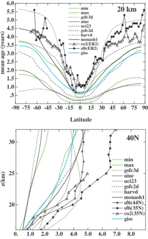
source of halogens. A linearly increasing tracer to diagnose transport was also in-cluded. This is presented in Fig. 1, which shows the age of air in the stratosphere calculated using the linearly increasing tracer in comparison with values derived from SF₆ and CO₂ observations (Andrews et al., 1999; Boering et al., 1996; Elkins et al., 1996; Harnisch et al., 1996) and values from other models (Hall et al., 1999). Clearly

10

the model’s air in the high latitude lower stratosphere is too young, a feature seen in most GCMs and even in CTMs driven by assimilated meteorological data (Scheele et al., 2005; Schoeberl et al., 2003). The annual mean residual vertical velocity in the model underestimates the maximum values seen in the UKMO analyses (Swinbank and O’Neill, 1994), and the region of upwelling extends too far poleward in the

South-15

ern Hemisphere, and to a much lesser extent in the Northern Hemisphere (Fig. 2). The model’s mean upwelling velocity is 35% slower than in the observations. However, the seasonal cycle shows the maximum upwelling occurring in the summer subtrop-ics in both hemispheres, in accord with Rosenlof (1995) and Plumb and Eluszkiewicz (1999). This simulation of the seasonality of tropical upwelling is a marked

improve-20

ment over that seen in the older GISS model II, which failed to reproduce the austral summer maximum entirely (Butchart et al., 20061). The model also simulates a local minimum in upwelling near the equator, a feature seen in most GCMs but not in pre-vious GISS models (Butchart et al., 20061). The underestimate of upwelling velocities indicates that air reaches the high latitude lower stratosphere too easily via

merid-25

1

Butchart, N., Scaife, A. A., Bourqui, M., et al.: A multi-model study of climate change in the Brewer-Dobson circulation, Clim. Dyn., submitted, 2006.

(12)

ACPD

Full Screen / Esc

EGU

ional transport across the semi-permeable barriers in the stratosphere rather than via a Brewer-Dobson circulation that is too rapid.

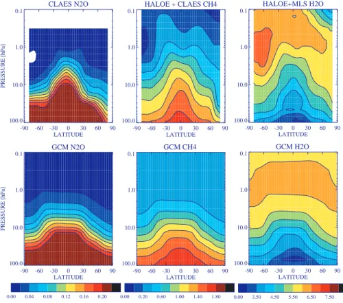
Consistent with these circulation biases, the model’s N₂O and CH₄ distributions are too broad compared with satellite climatologies from the Halogen Occultation Experi-ment (HALOE) and the Cryogenic Limb Array Etalon Spectrometer (CLAES) (Randel

5

et al., 1998) (Fig. 3). Also, the high mixing ratio values entering the stratosphere in the tropics do not penetrate to high enough altitudes before being chemically transformed. The distribution of CFCs in the model exhibits a similar shape. The weak meridional gradients in the distributions of these long-lived gases implies that transport across the subtropical and polar barriers is too rapid. Additionally, there may not be enough

10

downward transport within the polar vortex, as seen near the North Pole in Fig. 3. This appears to result from the underestimate of polar isolation which keeps the polar re-gion from cooling as much as it should, rather than biases in the overturning circulation given that the age of air is too short in the polar regions. In the interest of space, we concentrate on results for April, a month showing a “typical” ozone distribution neither

15

too close to the solstices nor drastically affected by polar heterogeneous chemistry. The distributions are similarly too broad in other months.

The model’s water vapor distribution in the stratosphere closely resembles the op-posite of the methane distribution up through ∼1 hPa. However, the water vapor near the tropical tropopause entry point is too low, leading to a negative bias throughout the

20

stratosphere. Given the extremely high sensitivity of water vapor to temperature and convective mixing in this region, the bias in water reflects only a small underestimate of temperature or overestimate of convective drying. As in observations, values increase by roughly 3 ppmv from the tropical tropopause to the upper stratosphere at 2 hPa. However, the model’s meridional gradients in stratospheric water are again too weak

25

and the stratopause region water values are too low, both features being consistent with the circulation-induced biases in the methane distribution. Water vapor mixing ra-tios decrease below 5.5 ppmv at about 0.2–0.3 hPa, as in observations, however this mesospheric loss takes place at all latitudes in the model but only near the springtime

(13)

ACPD

Full Screen / Esc

EGU

pole in observations. This may indicate that chemistry above the model top influences those layers, or that the current parameterization of mesospheric photolysis needs to be improved. Future work will explore this region further. The seasonality of water vapors entry into the stratosphere is simulated reasonably well, with a clear “tropical tape recorder” signal seen in the water vapor distribution (Schmidt et al., 2005).

5

3.2 Ozone

The model’s annual cycle of column ozone and the difference with respect to observa-tions is shown in Fig. 4. The simulated distribution shows a broad minimum and little seasonality in the tropics, with greater ozone values and a larger seasonal cycle at high latitudes, in good agreement with observations. However, the model underestimates

10

the magnitude of the seasonal cycle at high northern latitudes, with too little ozone during the winter and too much ozone during the summer, and has a general positive bias over the Antarctic. The model’s column ozone is within 10% of the observed value throughout the tropics and subtropics and over most mid-latitude areas. High latitude differences are larger, in excess of 20% in some locations during some seasons.

15

There are two primary reasons for the high latitude biases apparent in Fig. 4. During the summer, high latitude temperatures in the ModelE GCM without chemistry exhibit a cold bias of ∼10◦C in the lowermost stratosphere (Schmidt et al., 2006). By slowing down the rates of ozone destroying reactions, this contributes to an increasing positive ozone biases during summer and fall seen in both hemispheres. The second reason

20

is that the model’s transport of gases into high latitudes is in general too rapid in the lower stratosphere, with the subtropical and polar barriers being too permeable, as dis-cussed in Sect. 3.1. This transport bias contributes to the underaccumulation of ozone in the Arctic during winter, and to the failure of the model to simulate lower ozone values over the Antarctic than at Southern Hemisphere mid-latitudes during fall and

25

winter, in both cases as air is not confined closely enough within the polar region. The model does produce a fairly reasonable Antarctic ozone hole. The timing is consistent with observations, as is the depletion relative to the wintertime values, though the

(14)

min-ACPD

Full Screen / Esc

EGU

imum values are too large as those winter starting values are too large (as discussed previously).

Figure 5 presents the April zonal mean ozone distribution in the model and from the Microwave Limb Sounder (MLS) and HALOE instruments. Clearly the Arctic distribu-tion is too closely centered around 10 hPa, similar to middle latitudes, consistent with

5

an underestimate of downward transport within the polar vortex and too much mixing across the vortex boundary. The Southern Hemisphere polar vortex similarly shows too much ozone from about 10–5 hPa and contours of large ozone mixing ratios that extend too far poleward from the mid-latitude maximum. Ozone in the tropics is well-simulated, though the maximum ozone mixing ratio in the model is slightly less than

10

in observations. In fact, the simulation is generally of high quality in regions where ozone’s photochemical lifetime is short, suggesting that the model’s chemistry scheme works well and that biases are indeed largely related to transport.

In addition to examining the present-day stratospheric ozone climatology, sufficient data exists to allow evaluation of the sensitivity of stratospheric ozone to perturbations.

15

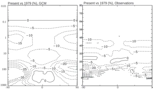
Observations from the Stratospheric Aerosol and Gas Experiment (SAGE) series of satellites have been used to calculate ozone trends over the period 1979 to 2004 (up-dated from Randel and Wu, 1999). We have performed a simulation using 1979 cli-mate and long-lived trace gas conditions (Table 3), and can then compare the modeled change from 1979 to the present with these observations, as shown in Fig. 6. Note that

20

our simulation did not include changes in emissions of short-lived tropospheric ozone precursors, as it was designed to isolate the impact of stratospheric ozone changes on the atmosphere. Qualitatively, the model captures the pattern of local maxima in ozone loss in both polar regions in the lowermost stratosphere and in the upper stratosphere and also simulates the local minimum in the tropical stratosphere around 25–30 km

25

altitude. Quantitatively, the model’s ozone trends are typically a few percent larger than those seen in the satellite record. This is especially true in the Arctic lower strato-sphere, though the uncertainty in the observed trends is very large as variability is high in this region. In the Antarctic lower stratosphere, the model’s trend is in fairly good

(15)

ACPD

Full Screen / Esc

EGU

agreement with the magnitude calculated from observations, though the largest deple-tion extends over a larger area, especially down into the troposphere. However, the values in the troposphere and near the tropopause in general are all more negative in the model since these simulations did not include increases in tropospheric ozone precursors. As seen in the runs that did include such increases, the troposphere

be-5

came more and more polluted during the twentieth century, which would account for the positive trends send in the lowermost portion of the SAGE data at mid-latitudes and in the tropics and also the smaller negative values seen at high latitudes.

To evaluate the lowermost stratosphere and troposphere, where satellite climatolo-gies do not yet exist, we have extensively compared modeled annual cycles of ozone

10

with a long-term balloon sonde climatology from remote sites (Logan, 1999). Annual cycles at several pressure levels are shown for selected sites in Fig. 7, while statistical comparisons with all sites are presented in Table 4. Results are included for simu-lations incorporating chemistry throughout the model domain and for simusimu-lations with tropospheric chemistry only. Values from the previous model II’ version are also shown

15

in the table for comparison.

The ozone values and annual cycles over a wide range of latitudes are reasonably well simulated (Fig. 7). The high latitude biases evident in the previous analysis of the total column are immediately apparent at the uppermost sonde levels, however. The full chemistry version underpredicts wintertime ozone at 125 hPa at both Resolute and

20

Hohenpeissenberg, and overpredicts at Lauder and especially at Syowa. Interestingly, the depth of the springtime ozone hole over Syowa is reproduced fairly reasonably. The biases have only a minor effect on lower altitudes at most locations, with the ex-ception of Syowa where they persist clearly through at least 500 hPa. The shape of the seasonal cycle is generally well reproduced in the model, with maximum and minimum

25

values typically falling at the correct time of year. There is clearly an underestimate of ozone in the tropical upper troposphere at Natal, but this is not the case at other locations.

(16)

ACPD

Full Screen / Esc

EGU

that the new composition and climate model gives a substantially improved simulation in comparison with the older model II’ tropospheric chemistry model. Running the new model in tropospheric chemistry-only mode leads to a better match with observations at all levels, though especially those away from the surface. Using the full chemistry cal-culation, inherently a more difficult endeavor compared with prescribing stratospheric

5

ozone to exactly match observations, coincidentally leads to differences with respect to observations that are quite similar to those seen in the tropospheric chemistry-only model II’. However, this implies that at a level such as 125 hPa, in the stratosphere for many of the sites, the full chemistry model does a much better job for the low latitude sites for which this level is in the troposphere (consistent with the modelE tropospheric

10

chemistry-only performance). Transport from the stratosphere to the troposphere is substantially improved in the new modelE, as evidenced by the improvement in the tro-pospheric chemistry modelE versus II’. Thus the large positive bias in the full chemistry model at 300 hPa does not result solely from excessive downward transport, a major problem in previous GISS GCMs. It is at least partially attributable to the overestimate

15

of high latitude lower stratospheric ozone, especially in the Southern Hemisphere. A similar statistical comparison of the full chemistry run with sonde data leaving out the two high latitude sites Resolute and Syowa shows average differences in ppbv reduced from 34.7 to 23.7 at 300 hPa, from 45.7 to 37.0 at 200 hPa, and from 83.2 to 75.8 ppbv at 125 hPa, while at lower levels, there is little effect. This demonstrates that, as

ex-20

pected, a fair amount of the discrepancy with observations arises from the model’s high latitude biases. However, some excessive downward transport may still be occurring, which is partially masked in the tropospheric chemistry-only run by the negative bias at 200 hPa. The large 300 hPa positive bias is thus not present in the modelE tropo-spheric chemistry-only run. Aside from this large positive bias (31%), biases at other

25

levels are generally quite small, with values of 12% or less (and often 3% or less) at all other levels for both the full chemistry and tropospheric chemistry-only simulations. The GISS tropospheric-only chemistry model participated in the ACCENT/IPCC AR4 assessment of chemistry models, which included an evaluation of present-day

(17)

simula-ACPD

Full Screen / Esc

EGU

tions against this same ozonesonde climatology. In comparison with the other models, the GISS model performed quite well, with a root-mean-square (rms) error value of 6.3 ppbv compared with a range of rms error values of 4.6 to 17.8 ppbv (Stevenson et al., 2006).

An additional simulation identical to the tropospheric chemistry-only run except

in-5

cluding heterogeneous reactions on dust surfaces was also performed. The same statistical comparison of ozone fields with sonde data for that run shows reductions in the mean ozone concentration at those sites of 1.3% at 300 hPa, of 9.8% at 500 hPa, and of 1.0% at 950 hPa. Changes are 0.5% or less at 125 and 200 hPa. The reduction occurs primarily via removal of nitric acid on dust surfaces (see Sect. 3.3), which

re-10

duces the reactive nitrogen available for ozone production. The overall effect on ozone is mixed, with minor improvements in the model-data comparison at some levels and minor reductions in quality at others. The effect of the model’s liquid tracer budget has also been assessed. The inclusion of liquid tracers leads to an overall reduction in ozone due to enhanced removal of soluble species such as HNO₃(see Sect. 3.2). The

15

tropospheric ozone burden is reduced by 10 Tg (3%). The changes are not uniform, however, with ozone generally decreasing in the upper troposphere but sometimes increasing at lower levels. For example, in the same statistical comparison with son-des discussed above, the ozone concentration at those sites is reduced by 0.6 ppbv at 300 hPa, but increased by 1.6 ppbv at 500 hPa. This results from enhanced downward

20

transport of aqueous-phase HNO₃via advection and precipitation followed by evapora-tion. Overall the comparison with sondes generally changes by only about 1%, though at the 900 hPa level the difference between sondes and the model is reduced by ∼3% with the inclusion of the liquid tracer.

Surface ozone data is more widely available, and we compare modeled values with

25

measurements from 40 sites using the climatology of Logan (1999), based on data from many sources (Cros et al., 1988; Kirchhoff and Rasmussen, 1990; Oltmans and Levy, 1994; Sanhueza et al., 1985; Sunwoo and Carmichael, 1994). The model does a reasonably good job of matching the observed annual cycle at most sites, a sample

(18)

ACPD

Full Screen / Esc

EGU

of which is shown in Fig. 8. The results for the tropospheric chemistry-only simulation are fairly similar to those of our previous model (Shindell et al., 2003), consistent with the 900 hPa results shown in Table 4. There is some improvement at Reykjavik owing to the improved downward transport at high latitudes. At Northern middle latitudes, the simulation at Rockport is substantially improved, while that in the Northeastern US

5

is marginally better though the Hohenpeissenberg results are marginally worse. The surface ozone values in the full chemistry simulation are very similar to those in the tropospheric chemistry-only version, unsurprisingly. Interestingly, South Pole shows a substantial difference, with more wintertime ozone in the full chemistry run. While this improves the agreement with observations, it results from the overestimate of ozone in

10

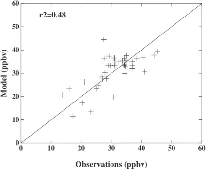
the Antarctic lower stratosphere. This does indicate that the model correctly transports stratospheric ozone anomalies all the way to the surface at South Pole. Comparing all 40 sites with the model’s values shows that the mean bias has decreased from +3.8 ppbv in model II’ to −1.4 ppbv in the tropospheric chemistry-only run and 0.6 ppbv in the full chemistry run. A correlation plot of the annual average surface ozone (Fig. 9),

15

however, shows that there is still substantial scatter despite the small mean bias. It is important to remember that the observations are primarily from remote sites, and that the model’s 4 by 5 degree grid boxes tend to include a mix of remote and urban locations over most continental regions, making the comparison somewhat imperfect.

It thus appears that the model generally does a reasonable job of reproducing

ob-20

servations throughout much of the atmosphere. The primary exception is the polar stratosphere, as discussed above, where values show biases up to about 25%. This is an important limitation, affecting the model’s usefulness in performing studies of polar ozone depletion, though the Antarctic ozone hole is fairly well represented. However, the model reproduced observations in the extrapolar regions quite well, and shows

25

especially good agreement near the surface and in the vicinity of the tropopause (Ta-ble 4). The latter is a key region for radiative forcing, and thus the results indicate that the model is useful for studies of how composition-climate interactions may affect climate and air quality.

(19)

ACPD

Full Screen / Esc

EGU

One area that has proved difficult to study in the past has been the response of STE to climate change. Without the inclusion of stratospheric chemistry, our previous stud-ies, and those of many other groups using tropospheric chemistry-only setups, were strongly influenced by the definition of the upper boundary for chemistry. For example, if chemistry was calculated below a fixed level, part of the upper troposphere and

low-5

ermost stratosphere, a region where data is sparse, had to be prescribed, and odd gra-dients could be created across this arbitrary chemical boundary. If instead chemistry followed the tropopause, changes in the location of the tropopause could dramatically affect the results as ozone amounts changed from climatology to calculated values. This latter effect could create sources and sinks as a box was categorized alternately

10

in one region then the other. The new full chemistry model avoids these problems, and so we explore the issue of STE in some depth in Sect. 4.4. In preparation for this, we give the tropospheric ozone budget for the models discussed here initially calcu-lating the terms for the atmosphere below 150 hPa and using fluxes across this level (Table 5).

15

The tropospheric ozone burden of 379 Tg in the tropospheric chemistry-only model is quite similar to the 349 Tg burden in the previous model II’ tropospheric chemistry-only version. These burdens are very close despite a large change in dry deposition between the two models that resulted from the switch between the earlier surface flux calculation to one consistent with other climate variables in the new modelE. This

re-20

inforces the point we’ve made previously that only the STE value is reasonably well constrained from observations. These give a best estimate of 450 Tg/yr with a range of 200 to 870 Tg/yr for the cross-tropopause flux based on O₃-NO_ycorrelations (Mur-phy and Fahey, 1994), a range of 450–590 Tg/yr at 100 hPa from satellite observations (Gettelman et al., 1997), and a constraint from potential vorticity and ozone fluxes for

25

the downward extrapolar flux (∼80–100% of total downward flux) of 470 Tg/yr for the year 2000 (Olsen et al., 2003). Some analyses also provide estimates of the ratio of NH to SH downward flux, with the NH contributing 55% of the total in Olsen et al. (2003) and 57% in (Gettelman et al., 1997). The present-day model results are in good

(20)

agree-ACPD

Full Screen / Esc

EGU

ment with this value, with 57% of the downward flux in the NH (Table 6). The total STE values in the tropospheric chemistry-only model are consistent with the observational constraints. The full chemistry simulation has a larger value that is on the high side of the range from observations, owing to the excessive downward ozone fluxes at high Southern latitudes where ozone amounts are overestimated (the full chemistry STE

5

value at 115 hPa, our closest level to 100 hPa, is 578 Tg/yr). The other budget terms simply respond to balance the tropospheric abundance as chemistry is typically very rapid, making the system highly buffered and the other budget terms of limited value for model evaluation.

3.3 Nitrogen species

10

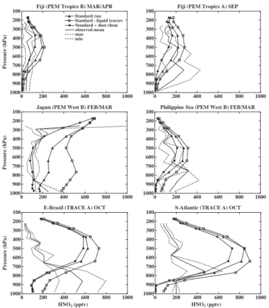
The model’s distribution of HNO₃ matches the location of maxima in the satellite ob-servations in both extratropical regions fairly well (Fig. 5). The area within the 9 ppbv contour is too large in the SH, however. Nitric acid can be formed by heterogeneous chemistry, and is therefore dependent upon aerosol and PSC surface areas and a pa-rameterization of particle growth and sedimentation. Since these are quite simple in

15

this model, it is not surprising that the abundance of HNO₃ does not match perfectly with observations. In the tropics, the level with maximum HNO₃occurs too low, consis-tent with the tropical upward transport being too slow and mixing across the subtropics being too rapid.

In the troposphere, the nitric acid simulation is in good qualitative agreement with

20

the limited available data, and is quantitatively much improved over previous results despite still being too large. Figure 10 shows nitric acid profiles from tropospheric chemistry-only simulations performed with and without the inclusion of heterogeneous chemistry on dust, and for a run without the use of the liquid tracer budget. These are compared with a variety of aircraft measurements (Emmons et al., 2000). In the

25

new simulations with or without heterogeneous chemistry on dust, the overestimate of HNO₃ typically seen in our earlier model II’ results has been reduced substantially in the new modelE, primarily as a result of the inclusion of a liquid tracer budget. The

(21)

ACPD

Full Screen / Esc

EGU

presence of a liquid tracer, allowing dissolved species to remain in the condensed phase for multiple timesteps, leads to global reductions in the abundance of soluble gases, with an overall reduction in the global HNO₃ burden of 5% and a reduction in the tropospheric ozone burden of 3%, as noted previously. The effect of the liquid budget is much larger for sulfur-containing species, some of whose burdens decreased

5

by 25–30% (Koch et al., 2006). In some locations where liquid water is abundant and long-lasting, quite large reductions occur (e.g. Japan in Fig. 10). Additionally, it is clear from the figure that heterogeneous chemistry on dust further improves the results in many locations (though not all). The overall model improvement is especially striking for Japan, where the liquid tracer and the removal of nitric acid on dust particles blowing

10

out from the Asian interior brings the modeled values down to observed levels. In contrast, profiles from model II’ or modelE without the liquid tracers or dust chemistry were roughly a factor of 5 too large in this area, while those from the modelE run without dust chemistry are a factor of 2 to 3 too large.

Similar comparisons of the vertical profiles of NO_x and PANs in the troposphere

15

show good agreement between the model and observations in most locations (not shown), similar to that seen in our previous model (Shindell et al., 2003). Analysis of the modeled NO_xsimulation in the stratosphere is complicated by the fact that the available climatologies from HALOE record sunrise and sunset NO and NO₂, but these species change rapidly during these times. The model’s monthly mean April NO_xshows a peak

20

of ∼12–13 ppbv in the tropics at ∼5 hPa, in reasonable agreement with the sum of NO and NO₂ in the HALOE sunrise measurements but somewhat lower than the sunset sum which is peaks at ∼18 ppbv. Given that the model values are a diurnal average, it seems reasonable that they should lie below some of the sunlit observations. Since nitrogen oxide abundances change so rapidly during sunrise and sunset, even a more

25

detailed comparison with the model results is likely to be inconclusive owing to the model’s half hour chemistry timestep.

The global annual average source of NO_x from lightning is 5.2 Tg N/yr in both the tropospheric chemistry-only and the full chemistry models. This source is calculated

(22)

ACPD

Full Screen / Esc

EGU

internally based on the GCM’s convection using parameterizations for total and cloud-to-ground lightning modified from (Price et al., 1997). The spatial distribution of light-ning agrees fairly well with observations (Boccippio et al., 1998), especially over land areas (Fig. 11). The model tends to overestimate lightning over SE Asia and Indone-sia, however. This leads to overestimates of the total flash rate of 5% during boreal

5

summer (JJA), and 17% during boreal winter (DJF) when lightning over South America is also overestimated.

The deposition of nitrogen in the model has been extensively compared with ob-servations as part of a wider model intercomparison (Lamarque et al., 2005). In that study the GISS model was run with several different sets of sea surface temperature

10

and sea ice boundary conditions. Comparisons were made with deposition measure-ments from acid rain monitoring networks in the NH. We summarize the results of those studies briefly here. In comparison against the North American network of deposition measurements (Holland et al., 2005), the GISS models showed correlations of 0.82 to 0.85 (regression over all points in the network against the equivalent model grid box),

15

comparable to the average of the 0.83 for the 6 different models in the intercomparison. The mean value was also in fairly good agreement at 0.20–0.25 gN/m2/year compared with an observed value of 0.19. For Asia, the GISS models’ correlations with the sin-gle year of available observations (see http://www.eanet.cc/) were 0.54–0.62, again consistent with the model average of 0.58. As in the other models, the GISS model

20

underestimated the mean flux by ∼50% however, perhaps reflecting the difficulties in-herent in comparison between large model grid boxes and point measurements in a densely populated area. It is also possible that the bias reflects and underestimate of nitrogen emissions from Asia. Inverse modeling using satellite observations sug-gests that Asian emissions are indeed underreported (Arellano et al., 2004; P ´etron et

25

al., 2004). Over Europe, the correlation coefficients in all the models, including GISS, dropped to much lower values (∼0.3), which may reflect the reduced sampling fre-quency or other biases in that network as discussed in Lamarque et al. (2005), but the mean values matched well with observations (0.27–0.38 GISS, 0.32 observed). Thus

(23)

ACPD

Full Screen / Esc

EGU

overall it seems that the GISS model does a good job in reproducing observed rates and distributions of nitrogen deposition fluxes in the NH regions where observations are considered reliable.

3.4 Halogens

The ClO maximum in the upper stratosphere is located at approximately the correct

al-5

titude and has the right magnitude at high latitudes in comparison with the MLS satellite climatology (Waters et al., 1996) (Fig. 5). The model underpredicts ClO in the tropi-cal upper stratosphere, however, while HCl (not shown) is overpredicted in this region. These features appears to result from the underprediction of water vapor in this region, which leads to a commensurate underprediction of OH and hence a positive bias in

10

the HCl/ClO ratio. ClO is reasonably well simulated in the polar regions, except for the underestimate of downwelling within the polar vorticies noted previously. During polar winter and spring, heterogeneous activation of reservoir chlorine to reactive species (ClO in the spring) is well captured.

The model’s chlorine nitrate distribution shows peaks at middle to high latitudes

15

around 15–30 hPa. In the winter hemisphere, the peak values just exceed 1 ppbv and are located at around 60–80 degrees, while in the summer hemisphere the peak values are below 1 ppbv and are located at mid-latitudes, in accord with CLAES observations. Distributions of most bromine species are similar to their chlorine analogues, with BrO_x most prevalent at higher altitudes and BrONO₂showing peaks in the lower stratosphere

20

towards the poles with a substantial seasonal cycle. In contrast to HCl, however, HBr makes up only a small fraction of reactive bromine throughout the stratosphere. 3.5 Reduced carbon species in the troposphere

Tropospheric hydrocarbons and carbon monoxide play similar roles in tropospheric chemistry. The model’s simulation of these species is generally similar to that of the

25

(24)

ACPD

Full Screen / Esc

EGU

methane, comparisons with the surface measurements of the NOAA GMD (formerly CMDL) cooperative air sampling network (Dlugokencky et al., 1994) (updated to 2000– 2004) show that the model overestimates the interhemispheric gradient slightly, and tends to put its maximum values more poleward in the NH than observed (Fig. 12). The very large uncertainties in methane’s sources, however, easily encompass the

5

model/measurement differences. Comparison of the model’s surface CO with the GMD surface observations shows good agreement in both magnitude and seasonality, as shown in Shindell et al. (2005), suggesting that the model’s OH fields are reasonably realistic. For CO, several years of near-global satellite data have also recently become available, allowing for a much more thorough evaluation of tropospheric chemistry

sim-10

ulations. We have evaluated our model against the MOPITT CO observations in de-tail, comparing global and regional simulations throughout the year at various altitudes within the troposphere (Shindell et al., 2005). The evaluation showed that the model was able to capture the geographic, vertical and seasonal variations of CO quite well. Monthly mean correlations against observations were typically in the range of 0.8–0.9,

15

with highest values (up to 0.95) during the boreal winter and spring and lowest val-ues (0.7–0.8, depending strongly on the emissions inventory used) during the boreal autumn biomass burning season (Shindell et al., 2005).

The simulation of methyl hydroperoxide is similar to that obtained in the previous model, which was in good agreement with observations (Shindell et al., 2003). The

20

model captures the observed distribution and seasonality of this important radical in-termediate over both remote and polluted locations. Though the available dataset is quite sparse, the good agreement between the model and the observations gives us confidence in the model’s hydrocarbon oxidation scheme.

Methane’s lifetime is primarily determined by the rate of its chemical oxidation by OH,

25

with smaller contributions from loss to soils and the stratosphere. For comparison with other tropospheric models, we compute the methane lifetime in the GISS tropospheric chemistry model using a prescribed loss to soils of 30 Tg/yr and a loss to the strato-sphere of 40 Tg/yr. The result is a lifetime of 8.48 years, in excellent agreement with

(25)

ACPD

Full Screen / Esc

EGU

the value of 8.4±1.3 years recommended by the IPCC TAR based on observations and modeling studies (Prather et al., 2001). Participating models in the IPCC AR4 chem-istry simulations produced methane lifetimes ranging from 6.3 to 12.5 years (Stevenson et al., 2006), so it is by no means a given that a model will match observations. Thus we believe the model’s simulation of OH is likely to be quite realistic, especially in the

5

tropics where the bulk of methane oxidation takes place. Further supporting this con-clusion, comparison of the model’s simulation of hydrogen peroxide, produced by the chemical combination of two HO₂ molecules, is in good agreement with observations as in our previous simulations (Shindell et al., 2003).

3.6 Aerosols

10

The simulation of sulfate aerosols has largely been discussed elsewhere (Koch et al., 2006), though in those simulations the aerosols were not coupled with chemistry. The influence of interactive chemistry and aerosols in this model has been investigated ex-tensively, however (Bell et al., 2005). The effects of coupling chemistry and aerosols, as opposed to running with off-line fields of oxidants prescribed for the aerosol simulation,

15

were fairly small. The overall correlation between the model’s sulfate simulations and surface observations decreasing slightly, from an r2 of 0.56 to 0.54 (Fig. 13), though correlations over some regions, including the US, improved. Note that the network of surface stations has very inhomogeneous coverage, with 174 locations in the NH but only 17 in the SH, and a paucity of data over Asia and over ocean regions. The new

20

composition and climate model also includes the effects of chemistry on the surface of mineral dust aerosols, as discussed in Sect. 3.3. The effects of mineral dust on sulfate has been described elsewhere (Bauer and Koch, 2005). The model includes simulations of carbonaceous, sea-salt and nitrate aerosols as well, though these do not directly influence the simulations of other trace species in the model and are described

25

(26)

ACPD

Full Screen / Esc

EGU

4 Climate change simulations

4.1 Experimental setup

As noted previously, one issue that we were not able to adequately address in our earlier studies of the interactions between composition and climate change was the response of stratosphere-troposphere exchange to altered climate states. The new

5

full chemistry version of the model can now be used to explore this issue, as well as changes within the stratosphere, NO_x from lightning that’s transported into the strato-sphere, etc. We have therefore run additional simulations using conditions appropriate for both the preindustrial era and estimates of possible future conditions (Table 3).

For the preindustrial, we have removed all anthropogenic emissions into the

tropo-10

sphere, and set long-lived greenhouse gases to 1850 conditions. For the future, simula-tions were performed setting long-lived gases to their IPCC SRES scenario A1B 2080 concentrations. Emissions of short-lived species were unchanged from the present-day for these runs. The year 2080 was chosen to give an idea of the potential 2100 response, as our simulations are for equilibrium while the transient case typically lags

15

the forcing by ∼20 years. Additional simulations used the IPCC SRES A2 scenario for 2100. These included changes to emissions of short-lived gases, primarily ozone precursors. They used 2100 values rather than 2080 for consistency with the short-lived emissions estimates and to allow for comparisons with other 2100 model studies. We refer to both simulations as 2100 runs for convenience hereafter. Companion

fu-20

ture simulations were performed to separate the effects of climate and chemistry in the future. For an A2 climate-only run, the future concentration of CO₂was prescribed, thus altering temperatures throughout the atmosphere, and future SSTs from an earlier run were specified. Compositions and emissions for reactive gases were unchanged from the PD. For the A1B case, the future composition used in the full A1B run was

25

provided to the chemistry, but not to the radiation. We refer to this as the A1B compo-sition run, and to the A1B run with climate change as the A1B compocompo-sition and climate run (as distinct from an emissions and climate run such as for A2, since emissions of

(27)

ACPD

Full Screen / Esc

EGU

short-lived gases were not changed).

All these simulations for past and future time periods were run using a mixed–layer (Q-flux) ocean to allow the climate to adjust to the imposed greenhouse gas forcing (ex-cept the A1B composition and A2 climate-only runs). In this setup, ocean circulation is prescribed for computational efficiency and therefore does not respond to climate

5

changes (i.e. heat convergence is prescribed while allowing SST to adjust). In order to have an appropriate comparison, a present-day simulation with a mixed-layer ocean was also performed. Initial conditions for the ocean were taken from earlier runs for the appropriate time periods, and then all simulations were run for several years to estab-lish climate (and the faster chemical) equilibrium, at least three and up to 10 depending

10

on how close the initial conditions were to the balanced state. Simulations were run from 20–40 years, providing at least 15 and often 30–35 years of post-spinup results for analysis. All simulations use solar minimum conditions (1986) to allow for comparison with companion solar maximum experiments to be performed later. As the influence of the solar cycle is small, about 1–2% in column ozone with a maximum impact of

15

∼3–4% in the upper stratosphere (McCormack and Hood, 1996), this introduces only a very minor bias into the model’s climatology.

4.2 Response to climate and emissions changes: preindustrial conditions

We first examine the changes between the preindustrial and present day simulations including both climate and emissions changes. The annual average zonal mean

tem-20

perature changes in the troposphere display a modest increase during this period, consistent with surface observations, while in the middle and upper stratosphere tem-peratures decrease substantially (Fig. 14). Ozone changes are clearly dominated by the increase in emissions. As in the tropospheric chemistry-only models, the bulk of the troposphere shows increased ozone amounts with maximum values in the NH

subtrop-25

ics. Unlike the tropospheric chemistry-only models, however, the SH poleward of about 45 degrees shows a reduction in ozone in the full chemistry simulations, reflective of the reduced influx from the stratosphere owing to Antarctic ozone depletion (Table 6).

(28)

ACPD

Full Screen / Esc

EGU

Though the model’s downward transport at high Southern latitudes is clearly too large based on the comparison with sonde data shown previously, the influence of strato-spheric ozone depletion extending down to the surface is seen in both the model and in observations (Oltmans et al., 1997). This leads to small (<5 ppbv) decreases in sur-face ozone in the SH poleward of about 45 degrees, which contrast markedly with the

5

large increases seen in the NH, especially over mid-latitude continental areas where they exceed 20 ppbv in some areas (Fig. 15). Tropical and NH extratropical fluxes of ozone across the tropopause show relatively small changes between the preindustrial and the present-day (Table 6), indicating that the change in SH extratropical STE is in-deed driven by composition changes rather than climate-induced circulation changes.

10

Changes in stratospheric ozone have a similar pattern to those calculated for 1979– 2000, but enhanced in magnitude. The spatial pattern of the stratospheric ozone losses corresponds closely to that of increased chlorine monoxide from the PI to the PD (Fig. 16). This is not surprising as it is well-known that increased chlorine has been the main driver of past stratospheric ozone losses (World Meteorological Organization,

15

1999). Stratospheric ozone has also been influenced by changes in the abundance of other radicals, with losses from increased NO_x and HO_x in some regions. In general there is more NO_xin the stratosphere, consistent with the increase in its primary source gas N₂O, however there is less NO_x in the uppermost tropical troposphere and in the lower to middle stratosphere over Southern mid-latitudes. Both regions also show an

20

enhancement of OH concentrations over this period, consistent with an overall increase in water vapor driven by increased surface temperatures and methane. The increased OH speeds the removal of NO_x into nitrogen reservoir species, accounting for the re-duced NO_xin these areas. The changes in both OH and NO_xare quite small, however, and little clear direct effect is seen on ozone. The cooler stratospheric temperatures

25

(Fig. 14) partially compensated for some of the enhanced catalytic losses by slowing down many temperature-sensitive chemical reactions.

The RF from ozone (tropospheric and stratospheric) is 0.34 W/m2from the PI to the PD. In the tropospheric chemistry-only model it is 0.37 W/m2(Shindell et al., 2005) (all

(29)

ACPD

Full Screen / Esc

EGU

RFs are instantaneous tropopause values). This implies a very small contribution to RF from stratospheric ozone change. This conclusion is consistent with results from the 1979 simulations as well. To show the effects of stratospheric ozone depletion on both the stratosphere and troposphere in the absence of other changes, we performed the 1979 run including PD emissions of short-lived gases that primarily affect the

tropo-5

sphere, as noted previously. Thus it is not intended to show the actual time evolution of the atmosphere. It shows decreases in most of the troposphere as well as the strato-sphere (Fig. 6). These are created by reductions in the flux of stratospheric ozone into the troposphere (Table 5), and thus maximize at middle to high latitudes. The simula-tion yields a decrease in the tropospheric ozone burden between 1979 and the present

10

that is roughly 80 Tg. This is considerably larger than the total PI to PD increase in the tropospheric ozone burden of 40 Tg, suggesting that stratospheric ozone losses have indirectly offset roughly 2/3 of the increase in the tropospheric ozone burden Such a result implies a substantial future increase in tropospheric ozone as the stratospheric ozone layer recovers, though, as noted previously, the downward flux of ozone at high

15

latitudes is too large in this model. Since the tropospheric ozone decreases that result from transport of stratospheric air are primarily at high latitudes they contribute com-paratively little to the RF, however. In comparison with the total PI to PD changes, those from 1979 to the PD contain 61% of the stratospheric ozone decline (Table 5). The to-tal RF due to the effects of stratospheric ozone changes from 1979 to 2000 on both

20

the troposphere and stratosphere is quite small, only −0.04 W/m2. This small value is consistent with other recent results with our model (Hansen et al., 2005), which found a value of −0.06 W/m2using the observed trends which are slightly larger than those cal-culated by the model in the crucial region near the tropical tropopause (Fig. 6). Over the full PI to PD period, the stratospheric ozone depletion was about 1.5 times as large as

25

during 1979–2000, a result in good agreement with earlier analyses based on historical data (Shindell and Faluvegi, 2002). Ozone losses prior to 1979 result from increases in methane and nitrous oxide as well as the initial input of CFCs. This then implies an overall negative forcing from stratospheric ozone depletion of about −0.06 W/m2 from