HAL Id: hal-01165529
https://hal.inria.fr/hal-01165529
Submitted on 17 Jan 2020
HAL is a multi-disciplinary open access
archive for the deposit and dissemination of
sci-entific research documents, whether they are
pub-lished or not. The documents may come from
teaching and research institutions in France or
abroad, or from public or private research centers.
L’archive ouverte pluridisciplinaire HAL, est
destinée au dépôt et à la diffusion de documents
scientifiques de niveau recherche, publiés ou non,
émanant des établissements d’enseignement et de
recherche français ou étrangers, des laboratoires
publics ou privés.
Deembedding of filters in multiplexers via rational
approximation and interpolation
Fabien Seyfert, Matteo Oldoni, Martine Olivi, Sanda Lefteriu, D. Pacaud
To cite this version:
Fabien Seyfert, Matteo Oldoni, Martine Olivi, Sanda Lefteriu, D. Pacaud. Deembedding of filters in
multiplexers via rational approximation and interpolation. International Journal of RF and Microwave
Computer-Aided Engineering, Wiley, 2015, pp.7. �hal-01165529�
Deembedding of filters in multiplexers
via rational approximation and interpolation
Fabien Seyfert
1, Matteo Oldoni
2, Martine Olivi
1, Sanda Lefteriu
1, Damien Pacaud
31
INRIA, Route des Lucioles - BP 93 - 06902 Sophia Antipolis Cedex, France 2
SIAE Microelettronica S.p.A., via M. Buonarroti, 21, 20093 Cologno Monzese (MI), Italy 3
Thales Alenia Space, 26 Av. J. F. Champollion, 31037 Toulouse, France
Received 20 September 2014;
ABSTRACT: In this paper we present a method to recover electrical parameters of filters embedded in a multiplexer for which scattering measurements are given. Unlike other approaches proposed for this problem, this method does not require a priori knowledge of the scattering parameters of the junction. This feature renders the procedure well suited for tuning purposes or for fault diagnosis. Technically the algorithm starts with a rational approximation step, in order to derive a rational representation of certain scattering parameters of the multiplexer. This representation is then used in a second step to identify the electrical model of each filter. This second step relies on a rational interpolation technique used to extract the filter’s responses. ©2014 Wiley Periodicals, Inc. Int J RF and Microwave CAE.
KEYWORDS: Diplexer, Filter tuning, Fault diagnosis, Deembedding, Rational
approximation, Padé interpolation
I. Introduction
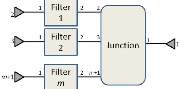
MICROWAVE multiplexers are present in nearly every transmission or reception unit of communication systems. The complex reciprocal loading effects of the filters connected via the junction (see Fig. 1) make their synthesis a difficult task: the latter commonly relies on computer-driven simulation, in the circuital and full wave domain, that are coupled to optimization methods [1]. The practical realization of such devices remains however a delicate matter, because of the inevitable dimension mismatch between the synthesized multiplexer and the realized one. The filters are therefore equipped with tuning elements (e.g. screws, irises) that need to be adjusted in the final manufacturing phase. When filters can be accessed and measured at their two ports, methods based on rational approximation have been developed ([2], [3], [4]) to extract the electrical parameters of the measured filter, and have led to efficient tuning procedures. By contrast, when tuning a multiplexer, detaching filters from the common junction is however hardly a possible or suitable option. Note also that in the early stages of a fault diagnosis procedure on a damaged device, the ability to identify precisely the malfunctioning filter(s), without disassembling the entire
Correspondence to: F. Seyfert; email: [email protected] DOI:
Published online: 00 Month Year in Wiley Online Library (wileyonlinelibrary.com)
multiplexer, might also be of great value. Concerning instead the design phase, moreover, a method to obtain the electrical parameters of the filters from a whole simulated multiplexer or manufactured prototype can be of great value to recognize mismatches with respect to the ideal model and thus improve the design.
For all these reasons, important efforts have been spent mostly on tuning techniques for multiplexers which rely only on external scattering measurements. Most of them are based on neural networks or on the minimization of a tuning criterion ([5], [6]), which however might suffer from the presence of local minima and usually give no real insight about the internal state of the hardware. Other approaches ([7]) have therefore been proposed in order to derive the filter’s electrical parameters: these however necessitate the additional knowledge of the junction’s scattering parameters, that might not be at hand in practice.
We describe here a method requiring the sole knowledge of the multiplexer’s external scattering measurements, the filter’s order and the coupling geometries (in-line, box section, triplets etc...) they implement. The procedure outputs are most of the electrical parameters of the filters up to the resonating frequency offsets of the resonators closest to the junction and their associated output couplings. It is also analytically proven that this is the best that can be done when starting from external measurements. From the latter our algorithm derives polynomial models of certain of the device’s scattering parameters, from which the rational scattering matrices of the filters can be extracted. Eventually the filter’s scattering matrices extracted in this way are synthesized in terms of electrical circuits of coupled resonators with the specified topologies, yielding the coupling matrix of each filter.
The core concepts of our method are described in the conference paper [8] whereas the present paper is enriched with a technical appendix which is essential for who wants to implement in practice the proposed procedure or understand in some details its functioning. Practical examples are expanded and one has also been added dealing with filters with finite transmission zeros embedded in a triplexer in order to demonstrate the versatility of the proposed approach.
II. Filter's Response Extraction
We consider the situation depicted in Figure 2:
a reciprocal filter is loaded on its second port by an unknown load
we have access to the reflection parameter S1,1 of this
system (filter+load) at port one of the filter
we know the filter's order N, its coupling topology and the location of its transmission zeros.
This section will try to answer the following natural question: under these circumstances, what can we say about the filter’s response itself? We call F1,1; F1,2; F2,2 the filter’s
scattering parameters, and L1,1 the reflection parameter of
the load. With these notations, the reflection parameter of the overall system expresses as:
2 , 2 1 , 1 1 , 1 2 2 , 1 1 , 1 1 , 1
1
)
(
F
L
L
F
F
S
(1)Evaluating the preceding expression at a transmission zero ωc of the filter is of interest in our situation, as it readily
yields:
)
(
)
(
)
(
)
(
1 , 1 1 , 1 1 , 1 1 , 1 c c c cS
F
S
F
(2)where the dot notation is used to indicate first derivatives with respect to ω, and the second equality can be easily proven by observing that F1,2appears squared in (1) and
vanishes at ωc thus nulling any further contribution to
) (
1 , 1 c
S
other than from Ḟ1,1(ωc). Eq. (2) further indicatesthat the values and the derivatives of the reflection
coefficient of the filter at one of its finite or infinite transmission zeros can be both inferred from those of the system’s reflection at the same point. Note that if ωc is a
zero of multiplicity m then the list of equalities (2) can be continued up to a derivative order 2m-1. This remark will be useful for transmission zeros at infinity: for example a filter of order N with an in-line coupling topology has a zero of order N at infinity. The rationality of F1,1= p/q leads us to
consider the following interpolation problem: supposing (ω1,... ωl) are all the filter’s transmission zeros of respective
order (m1,... ml) (Σmk = N), find all the polynomial pairs
(p, q) satisfying: ) ( ) ( } 1 2 ... 0 { }, ... 1 { () 1 , 1 ) ( k i k i k S q p m i l k
(3)The system (3) defines a rational interpolation problem, of Padé multipoint type [9], and can be solved classically using elementary methods from linear algebra. The system of equations (3) contains 2N equations compared to the 2N +2 unknowns corresponding to the coefficients of polynomials p and q. It is therefore no surprise that the following holds:
Proposition 2.1: All the polynomial pairs (p, q) of degree at most N that solve (3) form a two-dimensional space2. In particular there exist (p1, q1) and (p2, q2), such that, for all
complex numbers (α, β), the pair (p, q) defined as:
2 1 2 1 q q q p p p
(4)is a solution to (3). Moreover, any two pairs of distinct solutions satisfy 2 2 2 1 2 1
q
q
p
r
p
(5)with γ a complex number (depending on the special choice of the solution pair) r the transmission polynomial
k k m ks
r
)
(
.The lack of uniqueness of the identified filter's reflection coefficient is coherent with the following remark: one can always intercalate between the filter and the load (see Fig. 2) an arbitrary constant (independent on the frequency) chain matrix followed by its inverse, and this without changing the reflection parameter S1,1 of the system. The
filter's response is therefore at most recoverable up to the chaining of a constant chain matrix at its port two. The following proposition shows that this is the sole uncertainty on the filter's response:
Proposition 2.2: In the notations of proposition (2.1), and for any two pairs a=(p1, q1) and b=(p2, q2) solutions of (3),
the scattering matrix:
2 1 1 ,1
q
r
r
p
q
F
ab
(6)is a possible solution to our de-embedding problem, in the sense that:
Fa,b has ωk as transmission zeros
Fa,b is of McMillan degree at most N (its determinant is
a rational function of degree at most N)
It satisfies equation (2) at every transmission zero ωk.
2Strictly speaking, the assertion is true only generically (for almost
all), with respect to interpolation data Si
1,1(ωk)
Moreover, every solution in this sense to the de-embedding problem can be obtained like that. Eventually, for any two choices of solutions (a, b) and (c, d), Fa,b and Fc,d differ only
by a constant chain matrix connected on their second port. In order to access the electrical parameters of the filter we need now to consider circuital realizations of the derived rational scattering matrices. The considered circuital realization consists in the classical low-pass prototype [10], made of coupled resonators with a specified coupling topology. The following proposition indicates that most of the electrical parameters of the filter are recovered.
Proposition 2.3: Suppose that the filter has at most N-2 transmission zeros at finite frequencies, in order to admit a circuital realization with no source-load coupling [10]. Suppose that F is a possible solution of the de-embedding problem (in the sense of proposition 2.2) and admits a circuital representation characterized by a (N+2)×(N+2) coupling matrix M. Then any other solution F', also solution of the deembedding problem,admits a circuit representation with coupling matrix M' differing from M only for:
the frequency offset of the last cavity of the filter (nearest to the load), that is the value MN,N of the
coupling matrix;
the value of the output coupling represented by MN,L in
the coupling matrix (see [10]).
The preceding proposition, for which a proof is sketched in Sect. VI-D, indicates that the uncertainty on the scattering matrix of the filter has a very localized impact on its circuital representation. This is coherent with the fact that this uncertainty weighs on the value of a constant chain matrix plugged at its output port.
III. De-embedding Filters from a Multiplexer
The problem of de-embedding filters from a multiplexer, when starting from external measurements, is in many aspects similar to the simplified situation considered in Sect. II. If we call G the scattering matrix of the multiplexer:
Each filter appears to be loaded at its second port by a component regrouping the remaining filters connected via the junctions
For all these sub-systems, composed of a filter loaded by an unknown component, the reflection at port 1 is known. For the first filter, it is for example given by the scattering parameter G2,2, for the second by G3,3 etc... The transmission zeros, for example of filter 1, are also
present in the transmission parameters G2,1, G2,3, G2,4...
As we will see, this property can be used to locate the transmission zeros.
The core idea of the de-embedding algorithm is to perform a line-wise rational approximation of the scattering measurement of G: we will detail it from the perspective of the de-embedding problem of filter 1.
We start with a rational approximation of the row [G2,1, G2,2, G2,3...]. The order of the rational approximation
is chosen so as to get a proper fitting of the measurements and is in general higher than the filter's order: an additional increase in degree is introduced to approximate the effects of the loading. If the filter is expected to have finite transmission zeros, they can be identified using the following remark: the finite transmission zeros of filter 1 are the common zeros of the transmission parameters G2,1, G2,3, ... (apart from unlikely situations where all the
filters have the same transmission zeros, or the junction itself has a transmission zero). Their locations can therefore be obtained by analyzing the common zeros of the numerators of the rational approximations of G2,1, G2,3,....
Eventually, the values and derivatives of the right-hand term of (3) will be provided by evaluating the rational approximation of G2,2. Extraction of coupling parameters is
then obtained following the procedure outlined in section II.
IV. Practical Examples
A. Simulated Triplexer
The first example is rather academical, as measurements are obtained from simulations. The considered triplexer is built from a 4-port manifold junction on which we connected 3 filters of degree 4, each implementing 2 transmission zeros thanks to a "quartet" coupling geometry. The triplexer is evaluated on a frequency band from 11.4 GHz to 11.6 GHz by means of full-wave simulations. All the scattering parameters of the filters too are therefore available for this test and they can be processed by a classical de-embedding technique [3] to provide a reference coupling matrix that we will confront with results obtained only from external simulated scattering parameters.
A rational approximation of the scattering parameters [G2,1, G2,2, G2,3, G2,4] is performed to de-embed filter 1: a
degree 5 is needed in order to obtain a relative error less than 1%. Note here that, for all considered scattering parameters, the rest of the system (junction+remaining filters) is filtered out, away from the filter's passband: this explains the very moderate order needed for the rational approximation here. Then two finite transmission zeros are identified from the common zeros of rational representations of G2,1, G2,3, G2,4. These and two additional
zeros at infinity are retained as the filter's transmission zeros. The procedure in Sect. II can then be applied using the rational approximation of G2,2 in order to obtain possible
characteristic polynomials of the filter and hence its scattering matrix. The latter is then realized as a circuit with the following coupling matrix in arrow form [10]:
0 835 . 0 0 0 0 0 835 . 0 240 . 0 619 . 0 0 167 . 0 0 0 619 . 0 027 . 0 620 . 0 001 . 0 0 0 0 620 . 0 100 . 0 716 . 0 0 0 167 . 0 001 . 0 716 . 0 086 . 0 979 . 0 0 0 0 0 979 . 0 0
that is to be compared to the one extracted directly from the scattering parameters of the filter:
0 071 . 1 0 0 0 0 071 . 1 070 . 0 624 . 0 0 174 . 0 0 0 624 . 0 002 . 0 622 . 0 001 . 0 0 0 0 622 . 0 094 . 0 718 . 0 0 0 174 . 0 001 . 0 718 . 0 086 . 0 974 . 0 0 0 0 0 974 . 0 0
As expected, our procedure recovers all filter's electrical parameters up to the frequency offset of the last cavity and the output coupling. Similar results were obtained for the two other filters.
B. Measured Diplexer
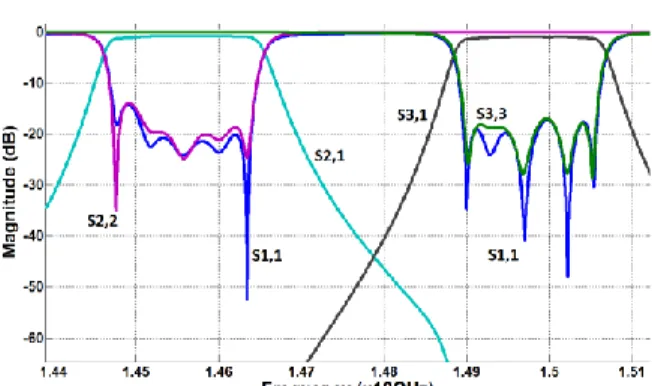
We now consider a real-world example, made of a manifold diplexer manufactured in one piece shown in Figure 3. The ports are WR62 rectangular waveguides. The lower-band filer was initially tuned to provide |S1,1|<-20 dB
from 14.478 GHz to 14.640 GHz, whereas the upper-band filter for |S1,1|<-17 dB from 14.896 GHz to 15.058 GHz (see
Fig. 4). The minimum loss on S2,1 and S3,1 is about 0.8 dB.
Both filters are of order 5 and implement an in-line coupling topology: all transmission zeros are therefore at infinity. To test our approach we ran several measurements of all the device's scattering parameters, while screwing in and out some tuning screws. Tuning screws entering laterally into the coupling windows between two cavities act like small capacitors: when screwed in, the corresponding coupling tend to augment. One can also expect the resonating frequencies of the adjacent cavities to be slightly affected by the coupling screws. In order to get a reference, we therefore ran a first identification of filter 1 and found the following coupling matrix:
0 091 . 1 0 0 0 0 0 091 . 1 136 . 0 860 . 0 0 0 0 0 0 860 . 0 145 . 0 617 . 0 0 0 0 0 0 617 . 0 032 . 0 631 . 0 0 0 0 0 0 631 . 0 012 . 0 839 . 0 0 0 0 0 0 839 . 0 006 . 0 015 . 1 0 0 0 0 0 015 . 1 0
We then screwed in the coupling screw between the 3rd and the 4th cavity, measured the diplexer (see Fig. 5) and identified the coupling matrix of the first filter as:
0 960 . 0 0 0 0 0 0 960 . 0 151 . 0 864 . 0 0 0 0 0 0 864 . 0 080 . 0 692 . 0 0 0 0 0 0 692 . 0 023 . 0 628 . 0 0 0 0 0 0 628 . 0 012 . 0 839 . 0 0 0 0 0 0 839 . 0 006 . 0 014 . 1 0 0 0 0 0 014 . 1 0
The predicted increase of the coupling M3,4 is confirmed by
the identification as well as a variation of the resonating frequency of the 3rd and 4th cavities. As explained in section
II, the identified elements M5,5 and MN,L should not be given
attention to. We ran other similar experiments, also altering screws located at cavities centre, and always found the identified matrices to be coherent with the performed action.
V. Conclusions
In this paper we presented a method to extract the electrical parameters of a multiplexer's filters through the sole knowledge of external scattering measurements. The method can be seen as an analogue, in the context of system identification, of Darlington's extraction procedure [11] used in the context of filter synthesis. The method was validated on practical examples and is suited for applications in the context of computer-assisted tuning and fault diagnosis or in the design and early prototyping. Although it has not been tested yet, application of the methodology to other complex devices combining filters accessible by only one of their ports seems promising.
VI. Appendix
A. Padé interpolation
The purpose here is to detail how the interpolation system (3) translates into a linear system of equations, and can therefore be tackled efficiently in practice. We consider one of the l interpolation series of the equation (3), w.l.o.g. the one occurring at ω1:
) ( ) ( } 1 2 ... 0 { () 1 1 , 1 1 ) ( 1
i i S q p m i (7)The latter specifies the value of the rational function p/q and of 2m1‒1 of its derivatives at the point ω1. Using the Taylor
expansion of S1,1 at ω1, this can be rephrased as:
Fig. 5:Response of the diplexer in Fig. 3 when the screw on the coupling between 3rd and 4th resonator of the lower filter was inserted by half a turn from the original (tuned) position. The lower edge of the lower band is clearly modified from Fig. 4 Fig. 4:Response of the diplexer in Fig. 3 when correctly tuned, used to extract the reference model
Fig. 3: Manufactured diplexer. Tuning screws are used to adjust coupling and resonating frequency of the cavities
2 1 0 1 2 1 1 1 ) ( 1 , 1 1 1 ) ( ) ( ! ) ( ) ( m i m i i O i S q p
(8)which, after multiplication by the denominator q implies,
2 1 0 1 2 1 1 1 ) ( 1 , 1 1 1 ) ( ) ( ) ( ! ) ( ) ( m i m i i O q i S p
. (9)By eq. (7), the left-hand term of (9) therefore vanishes at ω1
as well as its first 2m1‒1 derivatives. Differentiating the
latter j times (j<2m1) and evaluating it at ω= ω1 leads to,
} 1 2 ... 0 { 1 j m
j i i j i j q S i j p 0 ) ( 1 1 ) ( 1 , 1 ) ( 1) ( ) ( ) 0 (
(10) where )! ( ! ! i j i j i j is the binomial coefficient. If we set
N k k p p 0 and
N k k q q 0 , equations (10) express as 2m1homogeneous linear equations in the unknowns (pk), (qk).
The interpolation problem (3) amounts therefore to find the kernel of an homogeneous system of 2N linear equations in the 2N+2 unknowns (pk, qk).
In practice this can be tackled, for example, by a numerical procedure computing the singular value decomposition of a matrix (ex. svd() from Matlab). One can in fact define a column vector composed by the coefficients of p and q (both in decreasing order of power) as unknown quantity. Then, each eq. (10) can be written as a row of numerical coefficients multiplying the unknown vector to give 0. Thus the first transmission zero ω1 will result in 2m1 rows and,
similarly, 2mk rows will correspond to all the other zeros
ωk.The resulting matrix (M, 2N rows by 2(N+1) columns)
can be expressed by its SVD decomposition as USVT=M. The matrix S will include two null singular values in its diagonal, whose associated right vectors (corresponding columns of V) represent one set of coefficients of p and q each. Any linear combination of these solutions is also a valid solution of the interpolation problem.
We have presented here the elementary notions for Padé interpolation, showing how rational interpolation amounts to solve a linear problem and how it develops. For a survey about this well studied topic, see for example [12].
B. Sketched proof of Proposition 2.1
The first part of proposition 2.1 is a consequence of the preceding section, that transforms rational interpolation into solving a linear homogeneous system. The dimension of the solution space (here 2) is derived from the presence of 2N+2 unknowns when compared to 2N linear equations (which can be shown to be generically of full rank 2N). Now if p1/q1 and p2/q2 are two solutions to problem (3) we have:
which leads to
2 1
1 2 2 1 ( ) } ... 1 { mk k O q p q p l k
(12)This indicates that the polynomial p1q2-p2q1 has zeros of
orders 2mk in each of the ωk's. This polynomial is however
of order at most 2N (and Σmk=N) and it is therefore
proportional to the polynomial r2 of equation (5).
C. Sketched proof of Proposition 2.2
The assertion about the MacMillan degree of rational matrix Fa,b is a consequence of the divisibility of the
determinant of its numerator matrix by the common denominator q [13]. This holds by construction of the matrix Fa,b as defined by eq. (5). Eventually, if Ta,band Ta',b' are the
chain matrices associated to Fa,b andFa',b', straightforward
algebraic computations show that Ta,b· Ta',b' is a constant
chain matrix, proving the last assertion of the proposition. D. Sketched proof of Proposition 2.3
The retained filter model is here the classical low-pass model made of coupled resonators shown in Figure 6. The electrical equations governing this model are given in state-space form as follows:
2 1 2 1 2 1 a a D Cx b b a a B Ax x (13)
where a1, a2, b1, b2 are the I/O power waves and x is a
vector containing resonators voltages. The matrices A, B, C, D are defined in terms of the circuital parameters as follows:
0 0 0 0 0 0 , 1 , I D B C jM A C B jM jM C t L N S (14)
where M is the coupling matrix of the low-pass network and I is the 2×2 identity matrix. The scattering matrix of the network is given as:
D
B
A
I
s
C
S
(
)
1
(15)From what precedes, we know that we are able to recover the filter's scattering matrix S up to a constant chain matrix T connected at its second port (see Figure 7). We therefore derive a circuital representation of the system composed by the filter followed by the chain matrix T. To do this, we seek a state-space representation of the dynamical system having (a1, a3) as inputs and (b1, b3) as outputs. We first express
(a2, b2) in terms of (a3, b3) by means of the chain matrix T:
3 2 , 2 3 1 , 2 2 3 2 , 1 3 1 , 1 2 b T a T b b T a T a (16)
2 1
2 2 1 1 ( ) } ... 1 { mk k O q p q p l k
(11)Fig. 7:Filter with a constant chain matrix on port 2 Fig. 6:Low-pass prototype
and replace the latter in the state space form (13). Simple algebraic manipulation yields a state-space realization (A', B', C', D') of our overall system that expresses as:
D T T T T D C B C T T C T T T C B A A t 2 , 1 2 , 2 1 , 2 1 , 1 2 , 1 2 , 2 2 , 1 2 , 2 2 , 1 0 0 1 ' ' ' 1 0 0 1 ' :) , 2 ( ) 2 (:, ' (17)
The sparse form of matrices B and C implies that the perturbation B(:,2)·C(2,:) only impacts the term AN,N of the
dynamic matrix: it represents the frequency offset of the last resonator. For B' and C' the perturbed terms are also those related to the output coupling. The modification in D only affects the value at infinity of the reflection at port 2, and can be seen as a change of reference plan at this access. We have therefore derived a circuital realization of the perturbed filter (by means of T) which coincides with the original one up to the coupling MN,L and the offset MN,N. All
other electrical parameters of the filter can therefore be read out of a circuital realization of any matrix of Prop. 2.2.
An alternative circuital interpretation can be used to reach the same conclusions. In fact, any constant 2-port network can be represented as a Π network of admittances; the central series admittance is in turn equivalent to a shunt one between two equal and opposite admittance inverters. These two and their respective outer admittances can be converted into phase shifters just by adding residual shunt admittances in the center. The resulting model of a general frequency-independent network is therefore made by two phase shifters with an equivalent single shunt admittance in between. When such a general component is connected as in Fig. 7 to port 2 of a filter modeled as in Fig. 6, simple circuital transformations (Fig. 8) involving scaling and equivalencies allow to collapse the MN,L coupling with the
closest phase shifter; the effect of the shunt admittance can then be included into the obtained phase shifter to give an equivalent phase shifter cascaded with the outer one. The resulting phase shifter can be finally decomposed as an external phase shifter and an inverter with a shunt admittance in parallel with the last resonator. The external phase shifter represents the reference plane change, whereas the modified inverter accounts for the varied external coupling coefficient and the shunt admittance for the last resonator's shifted frequency. The rest of the filter, after this complete transformation, remains unaffected.
REFERENCES
1. M. Yu and Y. Wang, Synthesis and beyond, IEEE Microwave Magazine, vol. 12, no. 6, pp. 62-76, 2011
2. D. Traina, G. Macchiarella and J. Bertelli, Computer-aided tuning of GSM base-station filters - Experimental results, in Proc. IEEE Radio and Wireless Symposium, pp. 587-590, 2006 3. F. Seyfert, L. Baratchart, J.-P. Marmorat, S. Bila and J.
Sombrin, Extraction of coupling parameters for microwave filters: determination of a stable rational model from scattering data, IEEE MTT-S Int. Microwave Symp. Digest, vol. 1, 2003 4. V. Miraftab and R. R. Mansour, Fully automated RF/Microwave
filter tuning by extracting human experience using fuzzy controllers, IEEE Transactions on Circuit and Systems, vol. 55, no. 5, pp. 1357-1367, 2008
5. J. J. Michalski, Artificial neural network algorithm for automated filter tuning with improved efficiency by usage of many golden filters, Proc. 18th Int. Microwave Radar and Wireless Communications (MIKON) Conference, pp. 1-3, 2010 6. M. Yu and W. C. Tang, A fully automated filter tuning robots
for wireless base station diplexers, in Workshop on Computer-Aided Filter Tuning, IEEE International Microwave Symposium, Philadephia, Jun. 8-13, 2003
7. M. Oldoni, F. Seyfert, G. Macchiarella and D. Pacaud, Deembedding of filters' responses from diplexer measurements, Microwave Symp. Digest, IEEE MTT-S International, 2011 8. F. Seyfert, M. Oldoni, M. Olivi, S. Lefteriu and D. Pacaud,
deembedding of filters in multiplexers via rational approximation and interpolation, Microwave Symposium Digest (MTT), 2014 IEEE MTT-S International, pp. 1-3, June 2014 9. E. W. Cheney, Introduction to Approximation Theory, AMS
Chelsea, 1987
10. R. J. Cameron, R. Mansour and C. M. Kudsia, Microwave Filters for Communication Systems: Fundamentals, Design and Applications, Wiley, 2007
11. H. Carlin and P. Civalleri, Wideband Circuit Design, CRC Press, 1997
12. O. Salazar-Celis, Practical rational interpolation of exact and inexact data, Ph.D. dissertation, University of Antwerpen, 2008 13. T. Kailath, Linear Systems, Prentice Hall, 1979
Fig. 8: Circuital transformation to embed a constant chain matrix into a filter's output coupling; MN,L is implemented by the J-inverter whereas phase shifters by -ϕ blocks.
Fabien Seyfert Fabien Seyfert received the Engineering degree from the Ecole Superieure des Mines de St. Etienne, St. Etienne, France, in 1993, and the Ph.D. degree in mathematics from the Ecole Superierure des Mines de Paris, Paris, France, in 1998. From 1998 to 2001, he was with Siemens, Munich, Germany, as a Researcher specializing in discrete and continuous optimization methods. Since 2002, he has been a Researcher with the Institut National de Recherche en Informatique et en Automatique (INRIA), Sophia-Antipolis, France. His research interests are focused on the development of efficient mathematical procedures and associated software for signal processing including computer-aided techniques for the design and tuning of microwave devices.
Martine Olivi Martine Olivi was
born in France, in 1958. She got the engineer's degree from Ecole des Mines de St-Etienne, France, and the PhD degree in Mathematics from Université de Provence, Marseille, France, in 1983 and 1987 respectively. Since 1988, she is with the Institut National de Recherche en Informatique et Automatique (INRIA), Sophia Antipolis, France. Her research interests include: rational approximation, parametrization of linear multivariable systems, Schur analysis, identification and design of resonant systems. Detailed information and publications are available at http://www-sop.inria.fr/members/Martine.Olivi/
Damien Pacaud was born in France,
in December 1971. In 2001, he received the Ph.D. degree in Applied Mathematics and Scientific Computing from the University of Bordeaux 1, France. In 1996, he joined the CEG Center to develop powerful electromagnetic numerical techniques. In 2000, he joined IEEA (Paris) to develop RF software. Since 2001, he is in charge of Filters and Multiplexers studies and developments for spatial applications at Thales Alenia Space, Toulouse, France. His main area of interest concerns optimization and computer-aided design (CAD) processes for novel passive microwave products.
Matteo Oldoni was born in Milan,
Italy, in 1984 and obtained his B.Sc. degree in Telecommunications Engineering in 2006 from the Politecnico di Milano, Milan, Italy and his M. Sc. Degree in 2009 from the same Polytechnic with a thesis on the synthesis of microwave lossy filters. That was also the topic of a paper with which he received the Young Engineers Prize at the European Microwave Conference the same year. He received his PhD in Information Technology with a thesis on the design of microwave filters in 2012. He is currently a researcher at SIAE Microelettronica S.p.A, Milan, Italy and his activities deal mainly with filter synthesis and tuning algorithms and also to modeling applied to antennas and electromagnetics.
Sanda Lefteriu is currently an
Assistant Professor in the department of Computer Science and Automatic Control at Ecole des Mines de Douai in France. She received the B.Sc. degree from Jacobs University Bremen (formerly International University Bremen), Bremen, Germany, in 2006 and the M.Sc. and Ph.D. degrees in electrical and computer engineering from Rice University, Houston, TX, USA, in 2008 and 2011, respectively. She was an experienced Researcher within the framework of the Marie Curie project “CAE Methodologies for MidFrequency Analysis in Vibration and Acoustics.” She also held a Post-Doctoral position with the APICS Team of the INRIA Institute in Sophia Antipolis, France. Her research interests are in the areas of system identification, model-order reduction of systems arising in different engineering applications, and numerical linear algebra.