HAL Id: hal-01815326
https://hal.archives-ouvertes.fr/hal-01815326
Submitted on 13 Nov 2020
HAL is a multi-disciplinary open access
archive for the deposit and dissemination of
sci-entific research documents, whether they are
pub-lished or not. The documents may come from
teaching and research institutions in France or
abroad, or from public or private research centers.
L’archive ouverte pluridisciplinaire HAL, est
destinée au dépôt et à la diffusion de documents
scientifiques de niveau recherche, publiés ou non,
émanant des établissements d’enseignement et de
recherche français ou étrangers, des laboratoires
publics ou privés.
Super-luminous Type II supernovae powered by
magnetars
Luc Dessart, Edouard Audit
To cite this version:
Luc Dessart, Edouard Audit.
Super-luminous Type II supernovae powered by magnetars.
As-tron.Astrophys., 2018, 613, pp.A5. �10.1051/0004-6361/201732229�. �hal-01815326�
Astronomy
&
Astrophysics
https://doi.org/10.1051/0004-6361/201732229
© ESO 2018
Super-luminous Type II supernovae powered by magnetars
Luc Dessart
1and Edouard Audit
21 Unidad Mixta Internacional Franco-Chilena de Astronomía (CNRS UMI 3386), Departamento de Astronomía, Universidad de
Chile, Camino El Observatorio, 1515 Las Condes, Santiago, Chile e-mail: luc.dessart@oca.eu
2 Maison de la Simulation, CEA, CNRS, Université Paris-Sud, UVSQ, Université Paris-Saclay, 91191 Gif-sur-Yvette, France
Received 2 November 2017 / Accepted 18 January 2018
ABSTRACT
Magnetar power is believed to be at the origin of numerous super-luminous supernovae (SNe) of Type Ic, arising from compact, hydrogen-deficient, Wolf-Rayet type stars. Here, we investigate the properties that magnetar power would have on standard-energy SNe associated with 15–20 M supergiant stars, either red (RSG; extended) or blue (BSG; more compact). We have used a combination
of Eulerian gray radiation-hydrodynamics and non-LTE steady-state radiative transfer to study their dynamical, photometric, and spectroscopic properties. Adopting magnetar fields of 1, 3.5, 7 × 10¹⁴G and rotational energies of 0.4, 1, and 3 × 1051erg, we produce
bolometric light curves with a broad maximum covering 50–150 d and a magnitude of 1043–1044erg s−1. The spectra at maximum light
are analogous to those of standard SNe II-P but bluer. Although the magnetar energy is channelled in equal proportion between SN kinetic energy and SN luminosity, the latter may be boosted by a factor of 10–100 compared to a standard SN II. This influence breaks the observed relation between brightness and ejecta expansion rate of standard Type II SNe. Magnetar energy injection also delays recombination and may even cause re-ionization, with a reversal in photospheric temperature and velocity. Depositing the magnetar energy in a narrow mass shell at the ejecta base leads to the formation of a dense shell at a few 1000 km s−1, which causes a light-curve
bump at the end of the photospheric phase. Depositing this energy over a broad range of mass in the inner ejecta, to mimic the effect of multi-dimensional fluid instabilities, prevents the formation of a dense shell and produces an earlier-rising and smoother light curve. The magnetar influence on the SN radiation is generally not visible prior to 20–30 d, during which one may discern a BSG from a RSG progenitor. We propose a magnetar model for the super-luminous Type II SN OGLE-SN14-073.
Key words. radiation: dynamics – radiative transfer – supernovae: general – supernova: individual: OGLE-SN2014-073
1. Introduction
A large number of super-luminous supernovae (SLSNe) of Type II show unambiguous evidence for interaction with circum-stellar material (CSM;Ofek et al. 2007;Smith et al. 2007;Stoll et al. 2011). Because of the large kinetic energy in standard SN ejecta, the observed time-integrated bolometric luminosity can be explained by invoking ejecta deceleration by a massive and dense CSM. The absence of broad, SN-like, lines at early times and the presence of narrow lines over an extended period of time is unambiguous evidence that such an interaction takes place. Some Type II SNe, however, show no obvious signature of interaction despite having a luminosity a factor of 10–100 larger than standard SNe II at maximum, for example, SN 2008es or OGLE–SN14-073 (Gezari et al. 2009; Miller et al. 2009; Terreran et al. 2017). What is striking in these events is the presence of HI lines well beyond the time of maximum, with a spectral morphology that is analogous to Type II-SNe during the photospheric phase (Gutiérrez et al. 2017). This property excludes a large amount of56Ni as the power source of the light
curve because in that case, the emitting layers at and beyond bolometric maximum are necessarily rich in intermediate mass elements (IMEs) and iron-group elements (IGEs), as obtained in Type II SN models produced by the pair-production instability in super-massive H-rich stars (Dessart et al. 2013b).
An alternative power source to the interaction between ejecta and CSM is the injection of energy from a magnetized fast-spinning compact remnant (i.e. a magnetar). Magnetars may be
associated with a wide range of astrophysical events, including γ-ray bursts (Duncan & Thompson 1992;Usov 1992;Thompson et al. 2004;Bucciantini et al. 2008,2009;Metzger et al. 2011, 2015), super or even extremely luminous SNe (Kasen & Bildsten 2010;Woosley 2010;Bersten et al. 2016;Sukhbold & Woosley 2016), or SNe presenting anomalies in their light curves such as a double bump (Maeda et al. 2007;Taddia et al. 2018). In the context of super-luminous SNe, a fundamental feature of mag-netars is their ability to supply power with a large range of magnitudes and time scales without stringent requirements on the ejecta mass or composition. The envelope and core properties of the progenitor might take diverse combinations, in contrast to pair-instability SNe whose large production of56Ni can only
occur in a progenitor of huge mass (Barkat et al. 1967).
Magnetar power has been invoked to explain the double-peak light curve of SN 2005bf (Maeda et al. 2007; see also Taddia et al. 2018).Kasen & Bildsten(2010) demonstrated that some combination of magnetar field strength and initial spin period (as well as ejecta mass and kinetic energy) could explain the observations of the Type II SN 2008es (Gezari et al. 2009; Miller et al. 2009) and the type Ic SN 2007bi (Gal-Yam et al. 2009). More recently, a large number of Type Ic SLSNe have been discovered and followed photometrically and spectroscop-ically from early to late times. Their radiative properties favor a magnetar origin in a massive Wolf-Rayet progenitor (Inserra et al. 2013; Nicholl et al. 2013, 2014; Jerkstrand et al. 2017). In most of these SLSNe Ic, distinguishing between56Ni power and magnetar power can in fact be done from a single spectrum
taken around bolometric maximum (Dessart et al. 2012). While most simulations have assumed spherical symmetry, a few radiation-hydrodynamics simulations performed in two dimen-sions suggest the occurrence of strong Rayleigh-Taylor driven mixing in the inner ejecta, affecting the thermal and density structures of a large fraction of the ejecta, which may affect the emergent radiation (Chen et al. 2016;Suzuki & Maeda 2017).
In this paper, we present results from numerical simulations of magnetar powered SNe resulting from the explosion of a red-supergiant (RSG) or a blue-supergiant (BSG) star. In the next section, we present the numerical setup for the radiation hydrodynamics and for the radiative transfer calculations. We then present our results. In Sect. 3, we first discuss the influ-ence of the adopted energy-deposition profile. We then describe the impact of the chemical stratification on the bolometric light curve (Sect.4). In Sect.5, we present the light curve differences obtained for the explosion of a BSG and a RSG progenitor influ-enced by the same magnetar. Using a given explosion model from a RSG progenitor, we explore the diversity of light curves and ejecta properties resulting from a grid of magnetar fields and spin periods (Sect.6). In Sect.7, we discuss our model results in the context of observations. We present our conclusions in Sect.8.
2. Numerical setup
We used the Eulerian radiation hydrodynamics code
HERACLES (González et al. 2007; Vaytet et al. 2011) to simulate the influence of magnetar power on a small set of SN ejecta models. We first describe the code assumptions and set up, then the treatment of magnetar power, followed by the progenitor models employed, and finally the post-processing for spectral calculations. A summary of properties from our simulations (initial conditions and results) is given in Table1. 2.1. Numerical approach withHERACLES
For the radiation-hydrodynamics simulations with HERACLES, we assume spherical symmetry. This choice is most likely inad-equate to describe the complex geometry of this system, both on large scales (see, e.g.,Burrows et al. 2007;Bucciantini et al. 2009; Mösta et al. 2015) and small scales (Chen et al. 2016; Suzuki & Maeda 2017). Spherical symmetry has been assumed so far in all simulations of magnetar-powered SN light curves and we make the same simplification for convenience for the time being. We also employ a gray approximation for the radia-tive transfer (one energy/frequency group). In the 1D simulations of interacting SNe presented inDessart et al. (2015,2016), we used a multi-group approach because the radiation and the gas could be strongly out of equilibrium, which does not apply as much here. We adopt a simple equation of state that treats the gas as ideal with γ = 5/3 and a mean atomic weight ¯Aof 1.35. The thermal energy of the gas is a tiny fraction of the radiative energy so the neglect, for example, of changes in the level of excitation and ionization of the gas has little impact on either the radiative or dynamical properties. The changes in ioniza-tion are accounted for in the computaioniza-tion of the Rossland mean opacity so the electron scattering opacity, which is the main con-tribution to the total opacity, is accurately accounted for. The code distinguishes absorptive from scattering opacity. At each grid point, the absorptive opacity is obtained by subtracting the electron scattering contribution to the Rosseland mean opacity (see Dessart et al. 2015 for details on how we compute these opacities). We have opacity tables for up to five different compo-sitions, characteristic of a massive star envelope at core collapse.
Namely, we adopt the composition of the H-rich envelope, the He-rich shell, the O-rich shell, the Si-rich shell, and a shell dom-inated by IGEs. For simplicity, most of the simulations presented here adopt a composition with XH= 0.65, XHe= 0.33, and a solar
composition for heavy elements (again, this composition is only relevant for the computation of the opacities).
To better resolve the ejecta at smaller radii, we use a grid with a constant spacing from the minimum radius at ∼1013cm up to
Rt= 5 × 1014cm, and then switch to a grid with a constant
spac-ing in the log up to 1016cm. The grid is designed to have no sharp
jump in spacing at Rt. For the boundary conditions, we adopt for
both the gas and the radiation a reflecting inner boundary and a free-flow outer boundary. The bolometric light curves that we extract from theHERACLESsimulations are computed using the total radiative flux at the outer boundary. The light travel time to the outer boundary at 1016cm introduces a delay for the record of the emergent radiation, by at most 3–4 d.
Radioactive decay is ignored in the present work. 2.2. Treatment of magnetar energy deposition
We use the formulation of Kasen & Bildsten (2010) for the magnetar power as a function of time since magnetar birth: ˙epm= (Epm/tpm) /(1+ (t + δtpm)/tpm)2 (1) with tpm= 6Ipmc3 B2pmR6pmω2pm , (2)
and where Epm, Bpm, Rpm, Ipm and ωpm are the initial rotational
energy, magnetic field, radius, moment of inertia, and angular velocity of the magnetar; δtpmis the elapsed time since magnetar
birth at the start of theHERACLESsimulation; and c is the speed of light. We adopt Ipm= 1045g cm2 and Rpm= 106cm. We use
here the special case of a magnetic dipole spin down. At late times, the magnetar power scales as 1/(B2t2).
The term δtpm is about 105s in our HERACLES simulations
because we do not start at the time of explosion. Instead, we start from an already existing ejecta at about 1 d after magnetar birth. This corresponds to a time shortly before shock breakout in our RSG progenitor, and well after shock breakout in out BSG model (see next section).
In our simulations, we ignore the magnetar energy deposited during the first 105s that follow core bounce and the magnetar
birth. This energy corresponds to
Eneglected= Epm(1 − 1/(1+ δtpm/tpm)) . (3)
Eneglected increases with Epm and Bpm. For example, it
can be as much as 1.8 × 1051erg for Epm= 3 × 1051erg and
Bpm= 7 × 10¹⁴G (so about 60% of Epm), while it is merely
1.7 × 1048erg for Epm= 0.4 × 1051erg and Bpm= 1014G (so less
than a per cent of Epm). This neglect impacts moderately the
emergent radiation because the energy deposited prior to one day is mostly used to boost the ejecta kinetic energy while it is strongly degraded by ejecta expansion.
The energy-deposition scheme is presented in detail in Sect.3.
2.3. Progenitor models and initial conditions for the
HERACLESsimulations
We use two different models for the initial conditions in
Table 1. Summary of model properties for the progenitor, the ejecta, the magnetar, and some results at bolometric maximum obtained with the
HERACLESsimulations.
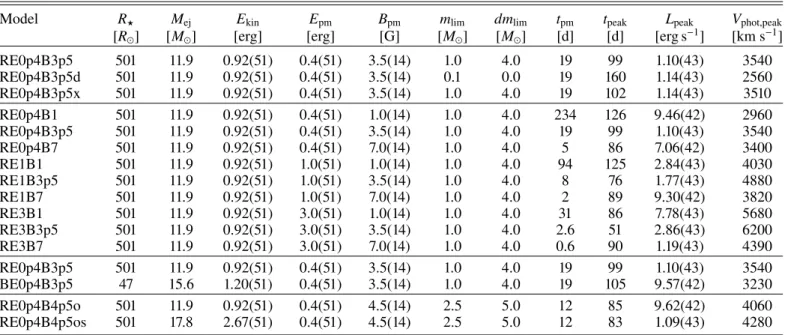
Model R? Mej Ekin Epm Bpm mlim dmlim tpm tpeak Lpeak Vphot,peak
[R ] [M ] [erg] [erg] [G] [M ] [M ] [d] [d] [erg s−1] [km s−1]
RE0p4B3p5 501 11.9 0.92(51) 0.4(51) 3.5(14) 1.0 4.0 19 99 1.10(43) 3540 RE0p4B3p5d 501 11.9 0.92(51) 0.4(51) 3.5(14) 0.1 0.0 19 160 1.14(43) 2560 RE0p4B3p5x 501 11.9 0.92(51) 0.4(51) 3.5(14) 1.0 4.0 19 102 1.14(43) 3510 RE0p4B1 501 11.9 0.92(51) 0.4(51) 1.0(14) 1.0 4.0 234 126 9.46(42) 2960 RE0p4B3p5 501 11.9 0.92(51) 0.4(51) 3.5(14) 1.0 4.0 19 99 1.10(43) 3540 RE0p4B7 501 11.9 0.92(51) 0.4(51) 7.0(14) 1.0 4.0 5 86 7.06(42) 3400 RE1B1 501 11.9 0.92(51) 1.0(51) 1.0(14) 1.0 4.0 94 125 2.84(43) 4030 RE1B3p5 501 11.9 0.92(51) 1.0(51) 3.5(14) 1.0 4.0 8 76 1.77(43) 4880 RE1B7 501 11.9 0.92(51) 1.0(51) 7.0(14) 1.0 4.0 2 89 9.30(42) 3820 RE3B1 501 11.9 0.92(51) 3.0(51) 1.0(14) 1.0 4.0 31 86 7.78(43) 5680 RE3B3p5 501 11.9 0.92(51) 3.0(51) 3.5(14) 1.0 4.0 2.6 51 2.86(43) 6200 RE3B7 501 11.9 0.92(51) 3.0(51) 7.0(14) 1.0 4.0 0.6 90 1.19(43) 4390 RE0p4B3p5 501 11.9 0.92(51) 0.4(51) 3.5(14) 1.0 4.0 19 99 1.10(43) 3540 BE0p4B3p5 47 15.6 1.20(51) 0.4(51) 3.5(14) 1.0 4.0 19 105 9.57(42) 3230 RE0p4B4p5o 501 11.9 0.92(51) 0.4(51) 4.5(14) 2.5 5.0 12 85 9.62(42) 4060 RE0p4B4p5os 501 17.8 2.67(51) 0.4(51) 4.5(14) 2.5 5.0 12 83 1.09(43) 4280
derives from a red-supergiant (RSG) model of a 15 M star
on the main sequence. At core collapse, it corresponds to a star with a total mass of 14.1 M , a surface radius of 500 R ,
a luminosity of 64 200 L . For the corresponding explosion,
the total ejecta mass is 11.9 M and the explosion energy is
0.92 × 1051erg (slightly different from the value inDessart et al.
2013abecause of remapping on a lower resolution Eulerian grid initially and trimming of the inner regions at small radii). The
56Ni yield is irrelevant since radioactive decay is ignored in this
study. The second model (lm18a7Ad ofDessart & Hillier 2010) derives from a BSG model of a 18 M star on the main sequence
(evolved at a metallicity of 0.008 rather than solar). At the onset of collapse, it corresponds to a star with a total mass of 17 M ,
a surface radius of 47 R , and a luminosity of 210 000 L . For
the corresponding explosion, the total ejecta mass is 15.6 M
and the explosion energy is 1.20 × 1051erg. Without magnetar power, these models reproduce closely the observed properties of the standard Type II-P SN 1999em and the Type II-peculiar SN 1987A (seeDessart et al. 2013a;Dessart & Hillier 2010for discussion and results).
These two models are used to cover the range of radii for Type II supernova progenitors, since the envelope extent is the fundamental characteristic that distinguishes the progenitors of Type II-Plateau and Type II-Peculiar SNe. Different progeni-tor main sequence masses and/or adopted wind mass loss rates would also impact the resulting observables of our magnetar-powered Type II SNe. This second aspect is left to a future study.
Because theHERACLES code is Eulerian, we start from an already existing ejecta rather than one at core bounce. For the RSG progenitor, we take the model at 105s after the explosion
trigger, which corresponds to about one hour before shock break-out. For the BSG progenitor we take the same starting time, but because of the reduced progenitor radius (i.e., 50 R ), this time is
well after shock breakout. Since we focus on relatively massive ejecta for which the rise time to bolometric maximum (excluding the initial shock breakout burst) is weeks to months, this ini-tial offset has little impact (see also discussion in the previous section).
We also need to specify the conditions between the outer edge of the progenitor/ejecta at 105s and the outer grid radius at 1016cm. For simplicity, we fill this volume with a
low-density low-temperature (set to 2000 K) material, reflecting a stellar wind mass loss rate of 10−6M
yr−1. A constant wind
velocity of 50 km s−1 is used for the RSG progenitor model,
and 500 km s−1 for the BSG progenitor model.1 These wind
velocities are approximate but have little impact on the results discussed here. Indeed, the ejecta/wind interaction contributes a few percent of the total bolometric luminosity. This contribution persists until the ejecta/wind interaction crosses the outer bound-ary of the Eulerian grid, at 125 d (50 d) in the simulations based on the RSG (BSG) progenitor.
Our model nomenclature is to use prefix “R” (“B”) to refer to simulations based on the RSG (BSG) models. We then append this prefix by values for the magnetar initial rotational energy and magnetic field. For example, simulation RE1B3p5 employs the RSG progenitor model, a magnetar initial rotational energy of 1051erg and a magnetic field strength of 3.5 × 10¹⁴G. In Sects.3
and4, we explore special cases for which we stitch an additional suffix (for example “x” or “d”).
2.4. Spectral simulations
We post-process the HERACLES simulations at the time when the SN reaches bolometric maximum, which is around 100 d after the start of the simulation for our sample. We use CMF
-GENin a steady-state mode and adopt the ejecta properties from
HERACLES (i.e., radius, velocity, density, temperature). Homol-ogous expansion is not assumed, which is why we read both the radius and the velocity. In most simulations, we adopt a uniform composition of a RSG star at death. We use mass fractions of 0.66 for H, 0.32 for He, 0.0019 for C, 0.004 for N, 0.008 for O, and use the solar metallicity value for heavier elements. The
CMFGENsimulations treat H, He, C, N, O, Na, Si, Ca, Ti, Sc, and Fe. The model atom includes HI, HeI-II, CI–III, NI–III,
1 Our BSG progenitor/explosion model is suitable for SN 1987A but
the adopted wind mass loss rate is too large and thus not strictly appropriate (see e.g.Chevalier & Dwarkadas 1995).
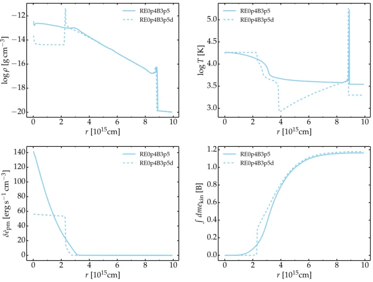
Fig. 1.Comparison of models RE0p4B3p5 and RE0p4B3p5d to test the influence of the radial profile used for the deposition of magnetar power. Ordered clockwise from top left, we show the radial variation of the mass density, temperature, local emissivity from magnetar power, and the cumulative kinetic energy integrated outward from the inner boundary, all at 116 d after the start of theHERACLESsimulation. Model RE0p4B3p5 spreads the magnetar energy over a large range of masses, while model RE0p4B3p5d deposits all the magnetar energy over the inner 0.1 M .
OI–III, NaI, SiII–III, CaII, TiII, ScII, and FeI–IV. For the starting level populations inCMFGEN, we adopt local thermody-namic equilibrium (LTE) and then evolve the non-LTE solution with the temperature fixed to what it was inHERACLES.
Evolving CMFGEN at a fixed temperature is not consis-tent but it provides a useful estimate of the emergent spec-tral energy distribution as well as the ionization, color, and line profile width/strength. During the photospheric phase, the ejecta is optically thick and lines do not dominate the luminosity. At late times, when the ejecta is optically thin, lines become the main coolant so that the LTE conditions assumed for the gas state inHERACLES are no longer suitable for a post-processing with CMFGEN. The CMFGEN simula-tions presented here are therefore limited to the photospheric phase. We use the (unambiguous) time of maximum for our comparisons.
3. Influence of energy deposition profile
We first start with the problematic issue of the treatment of mag-netar energy deposition. The newly-born hot magmag-netar probably emits high energy photons in the X-ray and γ-ray range as well as leptons (electrons and positrons). The lepton energy should be efficiently thermalized but high energy photons have a much
larger mean free path and may eventually deposit their energy far from their production site (they may even escape).
Secondly, as expected and demonstrated in recent 2D simu-lations (Chen et al. 2016;Suzuki & Maeda 2017), even if one assumes that the energy is deposited and thermalized at the ejecta base, this magnetar energy injection gives rise to strong Rayleigh-Taylor mixing in the inner ejecta. Rather than slowly diffusing out through the ejecta as it expands, the magnetar energy is more rapidly advected out by turbulent motions. In multiple dimensions, this turbulence prevents the formation of a fast moving dense shell in the inner ejecta, whose occurrence is an artifact of assuming spherical symmetry (Kasen & Bildsten 2010;Woosley 2010).
In this work, to mimic the effects of multi-dimensional insta-bilities seen in the simulations ofChen et al.(2016) andSuzuki & Maeda(2017), as well as the non-local nature of energy depo-sition of the magnetar, we deposit the magnetar energy over a range of mass shells rather than at the base of the ejecta. We use an energy deposition that has the same profile as the density, with an additional weight set to unity below a cer-tain mass limit mlim. In ejecta mass shells m beyond mlim, the
weight is either set to zero or to exp(−x2), where x = (m −
mlim)/dmlim(m is taken as zero at the ejecta base). The adopted
simulation. This is clearly very simplistic but it will allow us to gauge the impact on observables. In the future, it will be desirable to improve on this by performing multi-group radia-tive transfer (to solve for the transport of both high energy and low-energy photons), coupled with multi-dimensional hydrodynamics to describe adequately the contributions of energy transport by advection, diffusion, and non-local energy deposition (from high energy particles and photons with a large mean free path).
To test the influence of the magnetar energy deposition profile, we have run two simulations based on the RSG pro-genitor model and influenced by a magnetar with an initial rotational energy of 0.4 × 1051erg and a magnetar field strength of 3.5 × 10¹⁴G. In model RE0p4B3p5d, the weight is set to unity
below mlim= 0.1 M , and to zero above, that is the energy is
deposited over a narrow mass range of 0.1 M above the ejecta
base. In model RE0p4B3p5, the weight is set to unity below mlim= 1.0 M , and to exp(−x2) above, with dmlim= 4.0 M . The
corresponding volume integrated emissivity is then normalized to the magnetar power at the time.
We show a set of results for this test comparison in Fig.1, including the density, the temperature, the energy-deposition profile, and the cumulative kinetic energy versus radius (the time is 116 d, or 107s, for each simulation). In the case where
the magnetar energy is deposited in the inner 0.1 M of the
ejecta, the density profile exhibits a dense shell at ∼2.2 × 1015cm
and 2200 km s−1(the velocity profile, not shown, is essentially homologous for each simulation), with little mass below it. The temperature profile shows much more structure, with sharp variations in the cool regions above the photosphere. The temper-ature spike at large radii in both simulations corresponds to the shock with the surrounding low-density wind – the interaction power is small in comparison to the magnetar power.
The impact on the light curve is significant (Fig. 2). The time-integrated luminosity is greater by 1.5 × 1049erg in the
model RE0p4B3p5 characterized by a smooth/extended mag-netar energy deposition. This excess radiative energy in model RE0p4B3p5 yields instead an excess kinetic energy in the model RE0p4B3p5d. This is a one per cent difference since the total ejecta kinetic energy is ∼<1.2 × 1051erg (bottom right
panel in Fig. 1). The morphology of the light curve is also affected by the adopted treatment of magnetar energy deposi-tion. Model RE0p4B3p5d, in which the deposition is confined to the innermost ejecta layers and causes the formation of a dense shell, the light curve shows a pronounced bump at 150 d, which corresponds to the epoch when the photosphere recedes to those deep ejecta layers. Model RE0p4B3p5, in which the deposition is spread in mass space shows a smooth bolo-metric light curve. In this case, the onset of brightening also occurs ∼20 d sooner because of the energy deposition further out in the ejecta, at smaller optical depths. The simulations of Kasen & Bildsten(2010) do not show any jump in the light curve despite the formation of a dense shell at the base of their ejecta. This is probably because they adopt a fixed opacity, indepen-dent of ionization. Our models are H rich and the opacity varies steeply when H recombines, as occurs at 150 d in the dense shell formed in model RE0p4B3p5d.
While the energy deposition implemented in both models is artificial, the smooth and extended deposition profile adopted for model RE0p4B3p5 yields ejecta properties in better agreement with the 2-D simulations of Chen et al. (2016) and Suzuki & Maeda(2017), in particular with the lack of a dense shell in the inner ejecta. A similar effect on the density structure and on the resulting SN light curve is seen in radiation-hydrodynamics
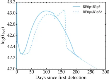
Fig. 2. Comparison of the bolometric light curve for simulations RE0p4B3p5 and RE0p4B3p5d, in which only the magnetar energy deposition profile differs (see Fig.1, and Sect.3for discussion). The glitch at 125 d occurs when the outer shock with the progenitor wind leaves the Eulerian grid at 1016cm. The broad bump at 150–170 d for
model RE0p4B3p5d occurs when the photosphere reaches the dense shell in the inner ejecta; the sharp drop at 170 d is when this dense shell becomes optically thin.
simulations based on 3D simulations of core-collapse SNe (Utrobin et al. 2017).
In the remaining of this work, we employ the same parametrized energy deposition profile as for RE0p4B3p5. Our magnetar-powered simulations will therefore tend to produce material distributed smoothly in velocity space down to very small values.
4. Influence of chemical stratification
We also tested the influence of chemical stratification on our results withHERACLES. InHERACLES, one can follow the evolu-tion of “scalars” from their initial distribuevolu-tion. In our Type II SN explosions, we approximate the ejecta composition using only the five most important species. We focus on the distribution of H, He, O, Si, and the initial56Ni (here,56Ni is just a tracer for
IGEs since we ignore radioactive decay). We renormalize the mass fraction to unity to correct for the missing species. The only impact of this chemical stratification on the numerical setup is through the opacity tables. Rather than using one table for an H-rich composition, we now use five tables to track the evolu-tion in mean atomic weight ¯Afrom the outer layers rich in H and He ( ¯A ≈1.35) down to the O-Si rich layers ( ¯A ≈17.0; this value depends on the progenitor/ejecta composition and the adopted mixing). We use the Rosseland mean opacity in our calculations so we account for the continuum opacity from bound-free and free-free processes, and from electron scattering opacity, as well as line opacity.
We have tested the impact of chemical stratification using model RE0p4B3p5x – model RE0p4B3p5 has a uniform com-position representative of the progenitor surface. We find no difference in dynamical properties between model RE0p4B3p5x and model RE0p4B3p5. The gas density matters but not the pre-cise distribution of this mass between different species/isotopes. Since we use the same equation of state for both models, we neglect the change in energy release from recombination and de-excitation of atoms/ions. However, the thermal pressure is
always a tiny fraction of the total pressure in SNe, and even more so in magnetar-powered SNe.
Figure 3 shows the bolometric light curves for models RE0p4B3p5x and RE0p4B3p5. The difference is negligible at early times, which is expected since more than half the ejecta is made of the progenitor H-rich envelope. At and after maximum, a small difference is seen, RE0p4B3p5x being first brighter and then fainter than model RE0p4B3p5. We interpret this results as arising from the earlier release of trapped radiation energy in model RE0p4B3p5x. The greater abundance of heavy ele-ments in model RE0p4B3p5x leads to a (modest) reduction in opacity, which makes the trapping of radiation less efficient. We use the Rosseland mean in our calculations so the reduction in opacity is driven by the reduction in electron-scattering opac-ity, and is not compensated by the greater metal line opacity at large ¯A.
5. Influence of the initial structure and radius: BSG versus RSG progenitors
Kasen & Bildsten (2010) considered a variety of magnetar properties (magnetic field and initial rotational energy), ejecta masses, and ejecta kinetic energies. However, they neglect the initial internal energy left by the shock passage (and that does not end up as kinetic energy for the ejecta), since this energy is typically much less than the energy released by a magnetar in a SLSN. One consequence in their simulation is a low predicted luminosity at times shorter than about the magnetar spin down time scale. In reality, during this early phase, an important source of energy is the shock deposited energy – it is even the dominant source of energy in the explosion of supergiant stars. Indeed, in supergiant stars, this energy is large, not strongly degraded by expansion, and allows even a standard SN II-P to radiate at 109L
for many days after the shock emergence. Accounting for
the large size of supergiant progenitors is therefore necessary to produce a consistent light curve prior to maximum (although the magnetar energy deposition may extend far out in the ejecta and affect the SN brightness very soon after explosion).
Here, we compare the predictions for the influence of a mag-netar (Epm= 0.4 × 1051erg, Bpm= 3.5 × 10¹⁴G) acting on a SN
ejecta that resulted from the explosion of a BSG and a RSG progenitor star. As discussed in Sect. 2.3, these models yield properties similar to SN 1987A and SN 1999em when evolved with no magnetar influence (Dessart & Hillier 2010; Dessart et al. 2013a).
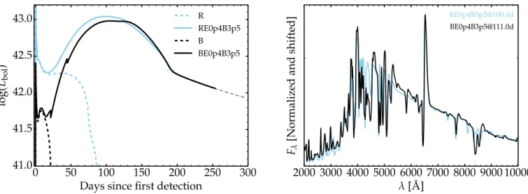
The left panel in Fig.4presents the bolometric light curve of models BE0p4B3p5 and RE0p4B3p5. The thick dashed lines correspond to the resultingHERACLESlight curve with no mag-netar and no56Ni (we ignore radioactive decay in this study).
For up to 20–30 d, the model luminosity is not influenced by the magnetar in our setup, but beyond that, the light curves of models BE0p4B3p5 and RE0p4B3p5 slowly converge and even-tually overlap soon after maximum. The resulting light curves have a bell shape morphology. As expected, the original star size matters only at early times, while at late times, the power sup-ply is so large that it overwhelms the slight differences that the two models may have had at explosion or at collapse. But the sizable differences at early times may allow to constrain the pro-genitor size, in the same fashion as for distinguishing SNe II-pec from SNe II-P (e.g., SN 1987A from SN 1999em, for which the differences at early times are well documented).
The right panel in Fig.4 shows the optical spectra for each model around the time of bolometric maximum. The differences
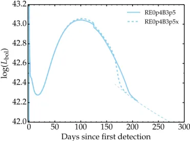
Fig. 3. Bolometric light curves computed with HERACLES for
models RE0p4B3p5 (homogenous composition with ¯A= 1.35) and
RE0p4B3p5x (chemically stratified and spanning ¯A= 1.35 up to 17). Allowing for a depth dependent abundance only affects the light curve after maximum, when the former (metal-rich) He-core material is pro-gressively revealed. The impact on the light curve is however minor here. The glitch at 125 d occurs when the outer shock with the pro-genitor wind leaves the Eulerian grid at 1016cm. The spectra for these
two models at maximum light are identical (hence not shown). This is because the spectrum then forms within the H-rich layers, and thus at the same composition in both models.
are marginal. It is important to notice that in such magnetar-powered SNe from H-rich stars, the spectra at maximum light show a typical Type II spectrum. In a model whose bolometric maximum is powered by the decay from a large mass of56Ni,
the optical spectra at bolometric maximum tend to show lines from IMEs, although HIlines may still be seen if the progenitor radius is huge (Dessart et al. 2013b).
6. Results for a grid of RSG-star explosions influenced by magnetar power
In this section, we present results for a grid of simulations in which the magnetar properties are varied. Using the RSG pro-genitor model, we cover magnetar initial rotational energies of 0.4, 1, and 3.5 × 1051erg (corresponding for our adopted neutron star to initial spin periods of 7.0, 4.4, and 2.6 ms) and mag-netic field strength of 1, 3.5, and 7 × 10¹⁴G. The magnetar spin down timescale covers from a day to several months (Table1; tpmscales as the inverse of B2pmEpm).
6.1. Bolometric light curves
We show the bolometric light curves for this set of models in Fig.5. The light curves all start at the same level, when the mag-netar influence has not yet been felt in the outer ejecta. This influence occurs sooner for a shorter spin down timescale tpm.
This depends also on the magnetar energy Epm in our
simula-tions but quantitatively, we need to be cautious since the energy released prior to 1 d is not accounted for in our simulations (this impacts our results for small values of tpm). The earlier the
bolometric light curve rises again, the faster is the rise to the bolometric maximum, which occurs in our set of simulations between 50 and 125 d after explosion. The bolometric maxi-mum spans the range 0.7–7.8 × 1043erg s−1. These values for
Fig. 4. Left: bolometric light curve computed withHERACLESfor models RE0p4B3p5 (RSG progenitor) and BE0p4B3p5 (BSG progenitor) under the influence of a magnetar (thick line) or not (thick dashed line). The thin dashed line corresponds to the magnetar power at >250 d. Prior to the influence of magnetar power on the emergent light, the luminosity stems primarily from shock deposited energy. It is at such early times that one may distinguish a BSG from a RSG star as the progenitor of a super-luminous SN. Right: maximum light spectra (around 100 d after explosion) for the two models shown at left.
Fig. 5.Bolometric light curves for the grid of magnetar-powered SN models based on the RSG progenitor. The glitch at 125 d occurs when the outer shock with the progenitor wind leaves the Eulerian grid at 1016cm. In AppendixA, we present light curves for model sets sharing
the same Epmor the same Bpm(see Sect.6for discussion).
tpeak and Lpeakare broadly consistent2 with the values obtained
from the analytic expressions (15) and (16) inKasen & Bildsten (2010). Beyond maximum, the bolometric luminosity falls onto the instantaneous magnetar luminosity (which then scales as the inverse of B2
pm) after a time similar to tpeak.
6.2. Energetics
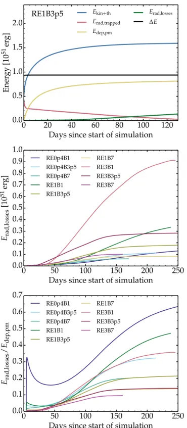
Figure6 illustrates the energetics in our simulation RE1B3p5. In the top panel, we show the evolution of the total gas energy Ekin+th (kinetic plus thermal contributions), the trapped
radia-tion energy Erad,trapped, the cumulative energy deposited by the
magnetar Edep,pm, and the cumulative radiative losses through
the outer boundary Erad,losses. We also plot the quantity ∆E ≡ 2 The broad and flat light curve maxima can complicate an accurate
estimate of the time of maximum.
Ekin+th+ Erad,trapped+ Erad,losses− Edep,pm, which should be
con-stant. This illustration shows that initially (the model is within hours of shock breakout) the trapped radiation energy is rapidly turned into kinetic energy while the supply of energy from the magnetar boosts both the trapped radiation energy and the ejecta kinetic energy. At 120 d, a little more than 1050erg has been
radi-ated to infinity, which is about ten times what this model would radiate in the absence of a magnetar (assuming that a represen-tative Type II SN, not influenced by a central source, radiates 1049erg over its entire lifetime). In this model RE1B3p5, the bulk of the magnetar energy has been channeled into ejecta kinetic energy, but yielding only a 60% increase in ejecta kinetic energy (not the factor of ten above for the radiative energy losses) over the value it would have had in the absence of a magnetar (at 120 d the magnetar in this model still has about 2 × 1050erg to radiate).
The middle and bottom panels in Fig. 6 illustrate how efficiently the magnetar energy is channelled into escaping radi-ation (referred to as Erad,losses). Nearly 1051erg is radiated away
in model RE3B1, while the rest of the models falls in the range 0.05–0.3 × 1051erg. The luminosity boost over a standard
SN II therefore goes from minor (5×) to very large (100×). When normalized to the current cumulative energy deposited by the magnetar, the most efficient “engines” are the magnetars with long spin down time scales, that is, those with a lower mag-netic field and/or a lower initial rotation energy (longer periods). These trends and quantities would not be significantly altered if we had started the magnetar energy deposition at the magnetar birth because it is only radiation emitted on a long time scale that boosts the bolometric luminosity of the SN (Kasen & Bildsten 2010).
6.3. Photospheric properties
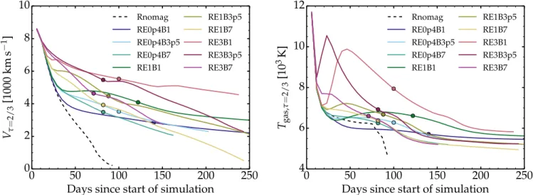
We show the evolution of the photospheric properties for our magnetar-powered SN models arising from the explosion of a RSG progenitor in Fig.7. Compared to the model without mag-netar (dashed line), the photospheric velocity is at all times larger, and by a large factor after 100 d since the no-magnetar model is by then optically thin. The effect illustrated here does not arise from a change in ejecta kinetic energy (which is essen-tially fixed after 50–100 d; see Fig.6and AppendixA) but stems
Fig. 6.Top: evolution of the various energy components in the RE1B3p5 simulation. We show Ekin+th, which sums the kinetic and thermal (i.e.,
gas) energy; Erad,trapped, which is the trapped radiation energy; Edep,pm,
which is the energy deposited by the magnetar; Erad,losses, which is the
radiative energy streaming out through the outer grid boundary; and ∆E ≡ Ekin+th+ Erad,trapped+ Erad,losses− Edep,pm, which tracks
conserva-tion of energy. The start of the simulaconserva-tion is 1.15 d in all simulaconserva-tions — any magnetar energy deposited prior to that is ignored. Middle and bottom: evolution of the radiative losses (middle) and of the fraction of the magnetar deposited energy that escapes as radiation as a function of time (bottom) for the magnetar-powered SN models based on the RSG progenitor. Additional illustrations are provided in AppendixA.
instead from the higher ionization of the ejecta. In the presence of a magnetar, the recombination is inhibited or delayed. The near plateau in the photospheric velocity after 50–100 d implies that the photosphere resides in a narrow range of ejecta mass shells (until >250 d in some models).
The photospheric temperature is larger at all times in the presence of a magnetar.3 In many models, this temperature
is close to the recombination temperature of hydrogen, which implies that the boost to the model luminosity is caused by the greater photospheric radius.
Interestingly, in the models with Epm > 1051erg, the
ini-tial decline of the photospheric temperature is halted at 10–40 d after the magnetar birth and the temperature starts rising again. In the models with the faster rotating magnetars (RE3B1 and RE3B3p5), the photospheric temperature reaches a maximum of about 10 000 K, which is sufficient to re-ionize hydrogen (in model RE3B7, the spin-down time scale is so short that most of the energy goes into work to accelerate the ejecta and the boost to Tphotis smaller than for models RE3B1 and RE3B3p5).
A non-monotonic evolution of the photospheric tempera-ture and of the location at maximum absorption in HeI5875 Å have been observed in the Type Ib SN 2005bf (Folatelli et al. 2006). This is consistent with the magnetar influence invoked to reproduce the light curve of SN 2005bf (Maeda et al. 2007). 6.4. Spectral properties at bolometric maximum
We conclude this section by discussing the optical spectra for our grid of models based on the RSG progenitor (Fig.8). This post-treatment of non-monotonic ejecta with CMFGEN is currently only possible during the photospheric phase so we choose the unambiguous time of bolometric maximum for this illustration.
The maximum light spectra shown in Fig.8 cover a range of optical colors, reflecting the range in photospheric tempera-ture (Fig.7). Bluer spectra appear like standard Type II SNe at early times, when the conditions at the photosphere are ionized or partially ionized. In model RE3B1 at 100 d, we recognize lines of HI, HeI, and NII, as in the earliest spectra for SN 1999em (Dessart & Hillier 2005,2006). Redder spectra appear like the standard Type II SNe at later times in the photospheric phase, when the conditions at the photosphere are partially neutral (and an H recombination front has formed;Dessart & Hillier 2011).
The line widths are, however, anomalously low for the SN luminosity. Indeed, the photospheric velocities at bolometric maximum are about 4000 km s−1 (Fig. 7 and Table 1), which
is standard for a Type II (Hamuy 2003), but the luminosity is up to 10–50 times larger than standard. In our choice of mag-netar properties, the energy released by the magmag-netar boosts primarily the radiation budget and affects little the kinetic energy (choosing a magnetar with a larger rotational energy and larger magnetic field would do the opposite). In doing so, it breaks the tight correlation between brightness and expansion rate inferred from the observation of Type II SNe (Hamuy 2003).
3 This holds except for model RE0p4B1, which is slightly cooler at the
photosphere. The energy released by the magnetar does not in princi-ple need to produce a higher photospheric temperature compared to the same model without a magnetar. Indeed, the influence of the magnetar may simply be to push the photosphere outward in mass/velocity space, while the photospheric temperature remains close the recombination temperature of hydrogen. In a SN II, the photosphere at the recombina-tion epoch coincides with the layer where hydrogen changes ionizarecombina-tion, from neutral to ionized. As long as there is such a recombination front, the photosphere is at roughly the same temperature, around 6000 K.
Fig. 7. Evolution of the photospheric velocity with time in theHERACLESsimulations for the RSG explosion model powered by a variety of magnetar energy and field strength. The colored dot on each curve corresponds to the time at which we compute the spectra shown in Fig.8.
Fig. 8. Model spectra computed with CMFGEN for the magnetar-powered RSG explosion models and corresponding to an epoch around bolometric maximum (see label for model name and post-explosion epoch). We stack the spectra vertically starting with the reddest at the bottom (model Re0p4B1) and progressing upward toward bluer spectra. Each flux spectrum is normalized at 10 000 Å and shifted vertically for visibility (the ordinate tick mark gives the zero-flux level).
Some observed Type II SNe, with no apparent sign of interac-tion, appear over-luminous for their expansion rate, for example, LSQ13fn (Polshaw et al. 2016) or SN 2006V (Taddia et al. 2012), and this may be a signature of a magnetar influence.
7. Comparison to observations
Few observations of super-luminous Type II SNe suggest a magnetar influence.Kasen & Bildsten(2010) propose a magne-tar with Bpm= 2 × 10¹⁴G, Epm= 5 × 1051erg (rotation period of
2 ms), and a H-rich ejecta of 5 M to explain the light curve of
SN 2008es (Gezari et al. 2009;Miller et al. 2009). Such a low mass ejecta is hard to fit within the context of an H-rich massive star progenitor so we leave this object aside for now.
Here, we choose a case that seems to be less ambiguous. We compare our simulations to the super-luminous Type II SN named OGLE-SN14-073 (Terreran et al. 2017), which exhibits a bolometric light curve similar to that of SN 1987A but brighter by a factor of ten and significantly broader (Fig.9, big black circles) – the time integrated luminosity up to >200 d is about 1050erg. The photospheric velocity inferred during the high brightness phase is about 6000 km s−1. Terreran et al. (2017) propose a RSG progenitor with an explosion model yielding a very large ejecta mass of about 60 M and kinetic energy of
12 × 1051erg. Their quoted uncertainties are however quite large.
We have compared our grid of models and found that RE0p4B3p5 and RE0p4B7 match closely the bolometric light curve. These models arise from an ejecta of 11.9 M and a kinetic
energy of about 1051erg, so 10 times less energetic and 5 times
less massive than proposed for OGLE-SN14-073 . Because their luminosity is too large at late times and too small at early times, we performed a new simulation (using the same initial ejecta model) with a higher magnetar field (Bpm= 4.5 × 10¹⁴G) and a
broader energy deposition profile (in order to hasten the magne-tar influence and produce a higher luminosity at early times – the alternative of a greater progenitor radius would also yield a greater brightness at early times).
In Fig. 9, we compare the bolometric light curve of this new model RE0p4B4p5o with the observations of OGLE-SN14-073, and include SN 1987A for reference. Model RE0p4B4p5o matches quite closely OGLE-SN14-073. How-ever, the photospheric velocity of these three models is about 4000 km s−1 at maximum, which is 50% lower than inferred
for OGLE-SN14-073. Scaling the initial density and velocity by 50%, as well as scaling the temperature by 22% (the model is pre-breakout hence half the total shock deposited energy is radiation, the other half is kinetic) we produce a new model RE0p4B4p5os (total mass of 17.8 M and a kinetic energy of
Fig. 9.Comparison of the bolometric light curves of magnetar-powered models RE0p4B4p5o (thick dashed line) and RE0p4B4p5os (thin line) with that inferred for OGLE-SN14-073 (empty circles;Terreran et al. 2017) and SN 1987A (empty squares;Hamuy et al. 1988). The origin of the x−axis is the time of the first signal detection at the outer grid boundary for the models (∼4 d after the start of the simulations), or the inferred time of explosion for the observations. We add the magnetar power of these two models (thin dashed line) and the radioactive decay power from 0.07 M
of56Ni (to match the nebular luminosity of SN 1987A; dash-dotted line). To power the nebular luminosity of OGLE-SN14-073 with radioactive
decay requires 0.47 M of56Ni (upper dash-dotted line).
2.67 × 1051erg). This choice of scaling is to increase the
veloc-ity while maintaining the same diffusion time (which scales as √
M/V). RE0p4B4p5os yields a similar light curve to OGLE-SN14-073. However, the photospheric velocity at bolometric maximum is only increased to 4280 km s−1, hence still signifi-cantly lower than the inferred value of 6000 km s−1 for
OGLE-SN14-073. Perhaps the kinetic energy is not underestimated and there is instead an error in inferring the photospheric velocity. The magnetar influence may affect line profiles such that the location of maximum line absorption occurs at a Doppler veloc-ity significantly greater than the photospheric velocveloc-ity value we report (which accounts only for electron scattering). Time dependence might also affect line profiles by preventing the formation of a steep recombination front as normally seen in standard Type II SNe (Utrobin & Chugai 2005;Dessart & Hillier 2008). Numerical explorations of magnetar-powered Type II SNe with CMFGENshow that spectral lines can remain very broad until late times, and broader than predicted using steady state (Dessart, in prep.). This aspect requires further study. But it seems likely that OGLE-SN14-073 is a unique Type II event, combining a massive and very energetic ejecta with a magnetar having Bpm= 4.5 × 10¹⁴G and Epm= 0.4 × 1051erg.
The ejecta corresponding to RE0p4B4p5os has a kinetic energy and mass greater than standard for a Type II SN but
less extreme than proposed byTerreran et al. (2017). Although not explicitly stated in their paper, the model of Terreran et al. requires 0.47 M of56Ni, while in our magnetar powered model
we assume no56Ni. The influence on the bolometric light should be similar since the power released in each process is simi-lar (see upper dash-dotted and dashed lines in Fig. 9). In the radioactive decay scenario, this56Ni mass makes sense since the
total decay energy from 1 M of 56Ni is ∼2 × 1050erg, and the
time integrated luminosity of OGLE-SN14-073 is about 1050erg.
The difference between a magnetar-powered model and a56 Ni-powered model is however non trivial when considering spectra and colors (Dessart et al. 2012). In OGLE-SN14-073, the pres-ence of a Type II spectrum at all times with little evidpres-ence for metal lines (Terreran et al. 2017) is hard to combine with the presence of a large progenitor CO core required to yield a large
56Ni mass. In explosion models powered by56Ni, the spectrum
formation region at the time of bolometric maximum is located in metal rich regions (Dessart et al. 2013b), which is in conflict with the observations of OGLE-SN14-073. If the power source is a magnetar, the ejecta composition may instead be dominated by H and He, which is compatible with the Type II spectrum observed at all times in OGLE-SN14-073.
At the time of bolometric maximum, the luminosity is a factor of 2 above the concomitant magnetar power in models
RE0p4B4p5o and RE0p4B4p5os – similar offsets are present in the set of simulations shown in Fig.5. An 80% offset is seen for SN 1987A between the bolometric maximum and the concomi-tant decay power from 0.07 M of56Ni. Arnett rule (Arnett 1982)
states that the peak bolometric luminosity should be equal to the power from which it derives (magnetar radiation, radioactive decay).
8. Conclusion
We have presented 1D gray radiation-hydrodynamics simula-tions of magnetar-powered Type II SNe performed with the code
HERACLES(González et al. 2007;Vaytet et al. 2011). Our simu-lations are based on BSG and RSG progenitors, which reproduce roughly the properties of SN 1987A (Dessart & Hillier 2010) and SN 1999em (Dessart et al. 2013a) if56Ni decay power (rather
than magnetar power) is accounted for. We adopt a power source from a magnetic dipole for convenience. In practice, the power radiated by such a compact remnant may not follow such a smooth evolution.
In our supergiant progenitors, the composition is dominated by H and He – the contribution in metals from the He core is secondary. In our magnetar-powered SN simulations, allowing for chemical stratification using five representative species (H, He, O, Si, and56Ni) makes little difference compared to
assum-ing a composition typical of a RSG H-rich envelope. Nearly all our simulations therefore assume a uniform H-rich composition. Furthermore, we mimic multi-D fluid instabilities seen in the simulations of Chen et al.(2016); Suzuki & Maeda (2017) by depositing the magnetar energy over a range of masses, rather than over a narrow mass range at the base. With this approach, the density and temperature structures remain smooth at all times, the light curves rise earlier and do not show a late time bump in the photospheric phase.
We find that early-time observations may help constrain the size of the progenitor star. Provided the magnetar influence does not start too soon, the SN luminosity arising from a BSG explo-sion is markedly lower than that from a RSG exploexplo-sion. By the time of maximum, the influence of the progenitor radius on expansion cooling is swamped by the large energy release from the magnetar. The light curves from the BSG and RSG magnetar-powered SNe overlap at and beyond maximum. Similarly, the optical spectra at maximum are similar and one would not be able to discern between the two progenitors from such a spectral information.
We then present a grid of models for RSG explo-sions influenced by a magnetar. For our set of magnetar field (1.0–7.0 × 10¹⁴G) and magnetar initial rotational energy
(0.4–3.0 × 1051erg), the resulting bolometric light curves reach a broad peak at 50–150 d after explosion with a power of 0.7–7.8 × 1043erg s−1. The fraction of the magnetar energy
chan-nelled into (UV-optical-infrared) SN radiation is higher for weaker field but in all cases the boost to the SN luminosity is sig-nificant (between a factor of 5 and 100 compared to a standard Type II SN). The magnetar influence delays the recombination of the ejecta and maintains the photosphere at a larger radius (in a mass shell located further out in the ejecta). In some cases, the magnetar energy deposition reverses the cooling and causes the photosphere to heat up after a few months. SN 2005bf exhibits a similar phenomenon (Folatelli et al. 2006), which is compatible with a magnetar origin (Maeda et al. 2007). The maximum light spectra are analogous to those of standard SNe II, with a range in colors that reflects the scatter in photospheric temperature (itself dependent on the heating efficiency of the magnetar). However,
the modest expansion rate and huge brightness of these magnetar powered SNe breaks the brightness/expansion-rate correlation observed in standard SNe II (Hamuy 2003).
Amongst super-luminous SNe II, it appears that OGLE-SN14-073 (Terreran et al. 2017) may be interpreted as a mag-netar powered SN. We find that our RSG model influenced by a magnetar with Epm= 0.4 × 1051erg and Epm= 4.5 × 10¹⁴G
yields a satisfactory match to the bolometric light curve, although our model underestimates the inferred expansion rate.
The main uncertainties in our simulations are the very approximate handling of the impact of multi-dimensional fluid instabilities (which will introduce clumping; Jerkstrand et al. 2017), the neglect of time dependence in the non-LTE solu-tion, and the neglect of non-thermal effects associated with the energy injection from the magnetar. Further modeling is there-fore needed, for example to test whether the line profile widths are broadened by the magnetar influence and time dependent effects, which could potentially lead to overestimating the ejecta kinetic energy and mass.
Acknowledgements.We thank Giacomo Terrreran for providing the estimated bolometric luminosity of OGLE-SN14-073. LD thanks ESO-Vitacura for their hospitality. This work utilized computing resources of the mesocentre SIGAMM, hosted by the Observatoire de la Côte d’Azur, Nice, France. This research was supported by the Munich Institute for Astro- and Particle Physics (MIAPP) of the DFG cluster of excellence “Origin and Structure of the Universe”.
References
Arnett, W. D. 1982,ApJ, 253, 785
Barkat, Z., Rakavy, G., & Sack, N. 1967,Phys. Rev. Lett., 18, 379
Bersten, M. C., Benvenuto, O. G., Orellana, M., & Nomoto, K. 2016,ApJ, 817, L8
Bucciantini, N., Quataert, E., Arons, J., Metzger, B. D., & Thompson, T. A. 2008,
MNRAS, 383, L25
Bucciantini, N., Quataert, E., Metzger, B. D., et al. 2009,MNRAS, 396, 2038
Burrows, A., Dessart, L., Livne, E., Ott, C. D., & Murphy, J. 2007,ApJ, 664, 416
Chen, K.-J., Woosley, S. E., & Sukhbold, T. 2016,ApJ, 832, 73
Chevalier, R. A., & Dwarkadas, V. V. 1995,ApJ, 452, L45
Dessart, L., & Hillier, D. J. 2005,A&A, 437, 667
Dessart, L., & Hillier, D. J. 2006,A&A, 447, 691
Dessart, L., & Hillier, D. J. 2008,MNRAS, 383, 57
Dessart, L., & Hillier, D. J. 2010,MNRAS, 405, 2141
Dessart, L., & Hillier, D. J. 2011,MNRAS, 410, 1739
Dessart, L., Hillier, D. J., Waldman, R., Livne, E., & Blondin, S. 2012,MNRAS, 426, L76
Dessart, L., Hillier, D. J., Waldman, R., & Livne, E. 2013a,MNRAS, 433, 1745
Dessart, L., Waldman, R., Livne, E., Hillier, D. J., & Blondin, S. 2013b,
MNRAS, 428, 3227
Dessart, L., Audit, E., & Hillier, D. J. 2015,MNRAS, 449, 4304
Dessart, L., Hillier, D. J., Audit, E., Livne, E., & Waldman, R. 2016,MNRAS, 458, 2094
Duncan, R. C., & Thompson, C. 1992,ApJ, 392, L9
Folatelli, G., Contreras, C., Phillips, M. M., et al. 2006,ApJ, 641, 1039
Gal-Yam, A., Mazzali, P., Ofek, E. O., et al. 2009,Nature, 462, 624
Gezari, S., Halpern, J. P., Grupe, D., et al. 2009,ApJ, 690, 1313
González, M., Audit, E., & Huynh, P. 2007,A&A, 464, 429
Gutiérrez, C. P., Anderson, J. P., Hamuy, M., et al. 2017,ApJ, 850, 89
Hamuy, M. 2003,ApJ, 582, 905
Hamuy, M., Suntzeff, N. B., Gonzalez, R., & Martin, G. 1988,AJ, 95, 63
Inserra, C., Smartt, S. J., Jerkstrand, A., et al. 2013,ApJ, 770, 128
Jerkstrand, A., Smartt, S. J., Inserra, C., et al. 2017,ApJ, 835, 13
Kasen, D., & Bildsten, L. 2010,ApJ, 717, 245
Maeda, K., Tanaka, M., Nomoto, K., et al. 2007,ApJ, 666, 1069
Metzger, B. D., Giannios, D., Thompson, T. A., Bucciantini, N., & Quataert, E. 2011,MNRAS, 413, 2031
Metzger, B. D., Margalit, B., Kasen, D., & Quataert, E. 2015,MNRAS, 454, 3311
Miller, A. A., Chornock, R., Perley, D. A., et al. 2009,ApJ, 690, 1303
Mösta, P., Ott, C. D., Radice, D., et al. 2015,Nature, 528, 376
Nicholl, M., Smartt, S. J., Jerkstrand, A., et al. 2013,Nature, 502, 346
Ofek, E. O., Cameron, P. B., Kasliwal, M. M., et al. 2007,ApJ, 659, L13
Polshaw, J., Kotak, R., Dessart, L., et al. 2016,A&A, 588, A1
Smith, N., Li, W., Foley, R. J., et al. 2007,ApJ, 666, 1116
Stoll, R., Prieto, J. L., Stanek, K. Z., et al. 2011,ApJ, 730, 34
Sukhbold, T., & Woosley, S. E. 2016,ApJ, 820, L38
Suzuki, A., & Maeda, K. 2017,MNRAS, 466, 2633
Taddia, F., Stritzinger, M. D., Sollerman, J., et al. 2012, A&A, 537, A140
Taddia, F., Sollerman, J., Fremling, C., et al. 2018,A&A, 609, A106
Terreran, G., Pumo, M. L., Chen, T.-W., et al. 2017,Nat. Astron., 1, 228
Thompson, T. A., Chang, P., & Quataert, E. 2004,ApJ, 611, 380
Usov, V. V. 1992,Nature, 357, 472
Utrobin, V. P., & Chugai, N. N. 2005,A&A, 441, 271
Utrobin, V. P., Wongwathanarat, A., Janka, H.-T., & Müller, E. 2017,ApJ, 846, 37
Vaytet, N. M. H., Audit, E., Dubroca, B., & Delahaye, F. 2011,J. Quant. Spectr. Rad. Transf., 112, 1323
Appendix A: Additional illustrations
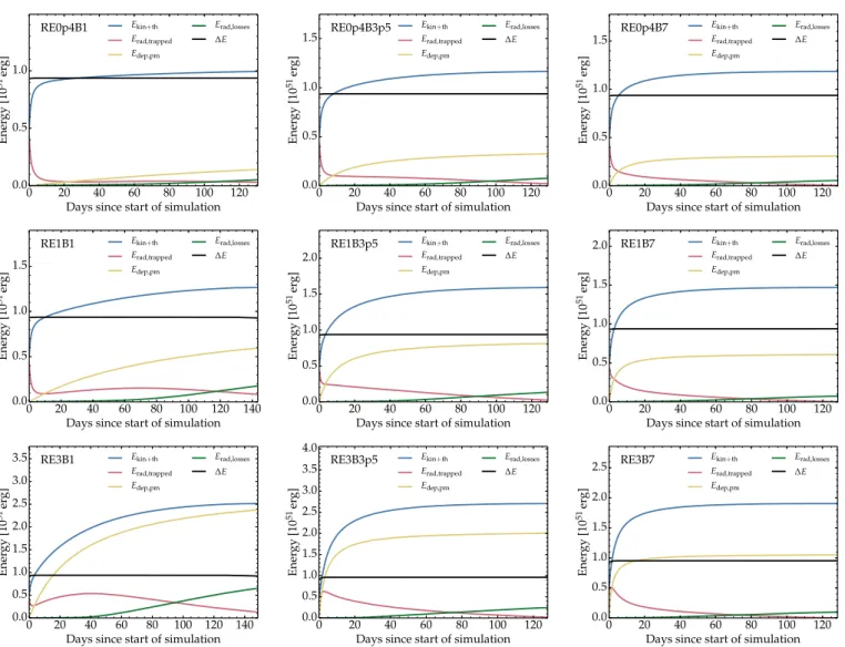
Fig. A.1.Evolution of the various energy components in theHERACLESsimulations. We show Ekin+th, which sums the kinetic and thermal (i.e., gas)
energy; Erad,trapped, which is the trapped radiation energy; Edep,pm, which is the energy deposited by the magnetar; Erad,losses, which is the radiative
energy streaming out through the outer grid boundary; and∆E, which is defined as Ekin+th+ Erad,trapped+ Erad,losses- Edep,pmand should be constant.
The start of the simulation is 1.15 d in all simulations — any magnetar energy deposited prior to that is not accounted for in the HERACLES
simulations.
In this appendix we provide additional illustrations for the models discussed in the main body of the paper. In Fig.A.1, we discuss the evolution of the various forms of energy on the grid, similarly to the top panel in Fig.6.
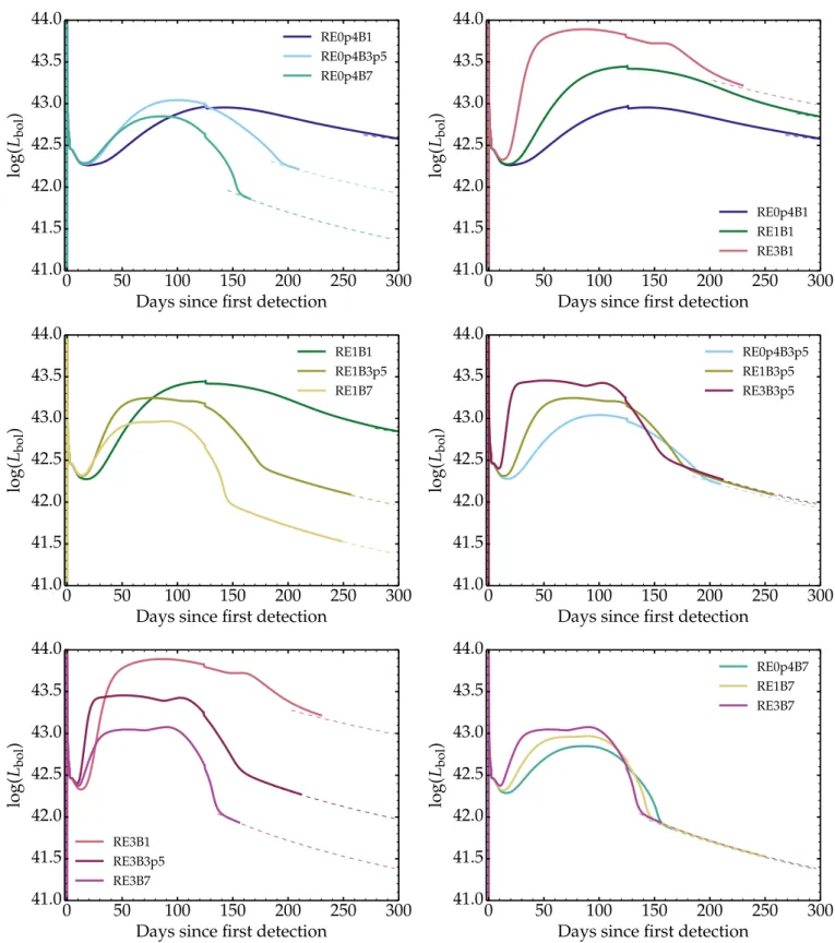
We also show in Fig.A.2the bolometric light curves for the magnetar-powered SN models discussed in Sect.6but this time
grouped by triads of the same magnetar initial rotational energy (but different magnetic field) or the same magnetic field (but different magnetar rotational energy).
Fig. A.2.Bolometric light curves fromHERACLESsimulations for the RSG progenitor. At ∼125 d, the shock between ejecta and progenitor wind leaves the grid and causes a slight glitch in the luminosity. In some models (e.g., RE3B7), the light curve shows a small bump at late times in the photospheric phase. This feature is associated with the dense shell that results from the dynamical influence of the magnetar power (even though we adopt a broad energy deposition profile; see Sect.3). Models with a higher initial magnetar energy and/or a higher magnetar field tend to produce a more massive dense shell and show this late light curve bump.