HAL Id: hal-01788222
https://hal-amu.archives-ouvertes.fr/hal-01788222
Submitted on 28 Oct 2020
HAL is a multi-disciplinary open access
archive for the deposit and dissemination of
sci-entific research documents, whether they are
pub-lished or not. The documents may come from
teaching and research institutions in France or
abroad, or from public or private research centers.
L’archive ouverte pluridisciplinaire HAL, est
destinée au dépôt et à la diffusion de documents
scientifiques de niveau recherche, publiés ou non,
émanant des établissements d’enseignement et de
recherche français ou étrangers, des laboratoires
publics ou privés.
improved terrestrial biosphere model: 2. Interannual
yields and anomalous CO 2 fluxes in 2003
P. Smith, Philippe Ciais, P. Peylin, N. de Noblet-Ducoudré, N. Viovy, Y.
Meurdesoif, Alberte Bondeau
To cite this version:
P. Smith, Philippe Ciais, P. Peylin, N. de Noblet-Ducoudré, N. Viovy, et al.. European-wide
simula-tions of croplands using an improved terrestrial biosphere model: 2. Interannual yields and anomalous
CO 2 fluxes in 2003. Journal of Geophysical Research, American Geophysical Union, 2010, 115 (G4),
�10.1029/2008JG000800�. �hal-01788222�
European
‐wide simulations of croplands using an improved
terrestrial biosphere model:
2. Interannual yields and anomalous CO
2fluxes in 2003
P. C. Smith,
1,2P. Ciais,
1P. Peylin,
3N. De Noblet
‐Ducoudré,
1N. Viovy,
1Y. Meurdesoif,
1and A. Bondeau
4Received 12 May 2009; revised 31 January 2010; accepted 21 May 2010; published 30 November 2010.
[1]
Aiming at producing improved estimates of carbon source/sink spatial and
interannual patterns across Europe (35% croplands), this work uses the ORCHIDEE
‐STICS
terrestrial biosphere model including a more realistic representation of croplands,
described in part 1 (Smith et al., 2010). Crop yield is derived from annual Net Primary
Productivity and compared with wheat and grain maize harvest data for five European
countries. Over a 34 year period, the best correlation coefficient obtained between
observed and simulated yield time series is for irrigated maize in Italy (R = 0.73). In the
data as well as in the model, 1976 and 2003 appear as climate anomalies causing a
≈40% yield drop in the most affected regions. Simulated interannual yield anomalies and
the spatial pattern of the yield drop in 2003 are found to be more realistic than the
results from ORCHIDEE with no representation of croplands. The simulated 2003
anomalous carbon source from European ecosystems to the atmosphere due to the 2003
summer heat wave is in good agreement with atmospheric inversions (0.20GtC, from
May to October). The anomaly is twice too large in the ORCHIDEE alone simulation,
owing to the unrealistically high exposure of herbaceous plants to the extreme summer
conditions. The mechanisms linking abnormally high summer temperatures, the crop
productivity drop, and significant carbon source from European ecosystems in 2003 are
discussed. Overall, this study highlights the importance of accounting for the specific
phenologies of crops sown both in winter and in spring and for irrigation applied to
summer crops in regional/global models of the terrestrial carbon cycle.
Citation: Smith, P. C., P. Ciais, P. Peylin, N. De Noblet‐Ducoudré, N. Viovy, Y. Meurdesoif, and A. Bondeau (2010), European‐wide simulations of croplands using an improved terrestrial biosphere model: 2. Interannual yields and anomalous CO2
fluxes in 2003, J. Geophys. Res., 115, G04028, doi:10.1029/2009JG001041.
1.
Introduction
[2] Crop yield is related to crop net primary productivity
(NPP), itself driven by climate and agricultural technology. Although agrotechnology has allowed a spectacular near threefold increase of NPP and yield over Europe and other regions over the past 40 years, climate fluctuations still exert a strong control on yield variability.
[3] For instance, the extended drought of 1976 in France
was accompanied by a drop of wheat yield, with values 16% lower than the 40 year trend value. More recently, the
summer drought and heat wave in 2003 caused a historical 20% reduction in maize yields in alpine regions (FAO ProdStat data, 2007, available at http://faostat.fao.org/site/ 567/default.aspx). Crop yield data inventories were long ago established to monitor food security and trade, to estimate food products prices, and more generally to provide input to agronomical research.
[4] The use of crop yield statistics to study the carbon cycle
emerged more recently. Local, regional, and national yield statistical data offer the unique advantage of long and rather homogeneous time series and provide uniform geographic coverage at large scales. Crop yield data were used in recent studies to evaluate models of NPP variability [Lobell and Asner, 2003; Bondeau et al., 2007], to assess the global dis-tribution of NPP [Goudriaan et al., 2001], to quantify the horizontal displacement of carbon by food trade circuits [Ciais et al., 2007], and to evaluate the large‐scale effect of climate extremes on plant growth [see, e.g., Ciais et al., 2005]. [5] In this study, we use country‐average crop yield
observed time series as well as surface CO2fluxes estimated
1Laboratoire des Sciences du Climat et de l’Environnement, Orme des
Merisiers, Gif‐sur‐Yvette, France.
2
Air Pollution/Climate Group, Swiss Federal Research Station Agroscope Reckenholz‐Taenikon, Zurich, Switzerland.
3
Institut National de la Recherche Agronomique, UMR BIOEMCO, Thiverval‐Grignon, France.
4
Potsdam Institute for Climate Impact Research, Potsdam, Germany. Copyright 2010 by the American Geophysical Union.
from atmospheric inversions to assess the performance of a terrestrial ecosystem model which specifically accounts for crops. The domain of the study is western Europe. Interannual yield model predictions are compared with the data given for two crop species (wheat, maize) in five countries (France, Spain, Italy, Germany and Austria) over the period 1972– 2003. The net land‐atmosphere CO2fluxes simulated by the
ecosystem model are compared over the whole domain with the surface fluxes derived from two global inversions.
[6] The coupled ecosystem‐crop model, called ORCHIDEE‐
STICS, is described in part 1 Smith et al. [2010], referred to in the following as“SMI09a”. The modeled crop phenology was tested against seasonal remote sensing greenness index observations. The mean simulated NPP was evaluated by using observed mean yield statistics, and uncertainties in allometric factors used to convert NPP into yield were shown to be crucial in the evaluation process.
[7] The research questions that are addressed in this
complementary study, roughly in sequential order, are [8] 1. To what extent can country‐level interannual yield
variations be used to evaluate the spatially explicit simulated NPP response to climate variability?
[9] 2. What mechanisms were involved in the crop
pro-ductivity changes during the 1976 drought and 2003 heat wave?
[10] 3. How do winter‐ versus spring‐type phenology and
irrigation help improve carbon balance simulation realism? [11] 4. How strongly does the overall crop productivity
drop contribute to the observed CO2source anomaly in the
atmosphere in 2003?
[12] 5. Can we use atmospheric inversions to falsify
modeled fluxes from the land surface and further improve the parameterization for instance of croplands?
[13] The discussions are provided at the end of each result
section (sections 3 and 4).
2.
Methods
2.1. ORCHIDEE‐STICS Modeling Framework [14] A comprehensive description of the modeling
strat-egy is provided in SMI09a; here, we only restate the main features. The improved model tested and applied in this study combines the terrestrial biosphere model ORCHIDEE [Krinner et al., 2005] (for vegetation productivity, water balance and soil carbon dynamics) and the generic crop model STICS [Brisson et al., 2003] (for phenology, irriga-tion, nitrogen balance and harvest). ORCHIDEE‐STICS relies on three plant functional types (PFT) for the repre-sentation of temperate agriculture: C3 winter‐type, C3 spring‐type and C4 crops. These PFT are parameterized as winter wheat, soybean and maize, respectively. Originally, ORCHIDEE alone uses only two “supergrass” C3 and C4 types covering the ground all year long, rain‐fed and growing mostly in summer. Agricultural practices needed for running STICS (sowing and harvest dates and crop variety) are fixed, in a first approximation, as being spatially homogeneous over Europe and representative of present technology. Crops are supposed to receive near‐optimum fertilizer and water (when irrigation is switched on) inputs. Several land cover data sets were combined to produce the vegetation map prescribing a fractional surface area to each
natural or agricultural PFT in each 0.5° × 0.5° grid cell. As in SMI09a, the model is forced by combined Climate Research Unit (CRU) [New et al., 2000] and National Centre for Environmental Predictions (NCEP) [Kalnay et al., 1996] climate variable fields and by the rising global atmo-spheric CO2concentration. Soil carbon pools were brought
to equilibrium for analyses of net carbon flux exchanges with the atmosphere via a spin‐up simulation of 10,000 years, repeating the 1970 year climate. The model European domain considered is the same as in SMI09a (−10° to 20° east and 35° to 55° north, 2,756,000 km2of land). The period covered by the simulations is also 1972–2003, including extensive droughts such as 1976 and 2003, which will be discussed further in this paper. The three simulations analyzed corre-spond to the use of ORCHIDEE alone (NoCROP) and both of ORCHIDEE‐STICS with irrigation (CROPi) and without (CROP). Outputs were archived at a daily time step. 2.2. Data Streams Used for Comparison With Simulations
[15] The interannual regional productivity distribution was
tested (via yield derivation) against national and subnational level crop harvest statistics. The continental‐scale seasonal CO2flux anomalies were compared with atmospheric
inver-sion estimates. These data sets are briefly described below. 2.2.1. Regional Harvest Statistics Interannual
Variations
[16] We used national statistics assembled by the FAO
(2007) data sets for crop yields and cultivated areas in Europe from 1961 to 2003. Only wheat and maize growing in France, Spain, Italy, Germany and Austria were considered. A long‐ term positive trend in grain yield can be observed for both crops in all countries. The average increase is of +0.15 t/ha/yr, equivalent to almost a tripling during the last 45 years. We are only interested here in the climate driven interannual vari-ability. Hence, the trend, which mostly reflects agricultural intensification and improved farmers’ practices [Gervois et al., 2008; Lobell and Asner, 2003; Goudriaan et al., 2001], was fitted with a linear curve and removed from the data. This means climate and CO2minor contribution to this
trend were ignored, although their effects are taken into account in the simulations.
[17] As described in the “From NPP to yield” section in
SMI09a, model yield was derived from annual NPP through four coefficients: root fraction, Harvest Index (i.e., harvested to aboveground NPP), grain humidity content and carbon content of Dry Matter.
2.2.2. Atmospheric Inversion Results
[18] No measurement of regional‐scale net carbon fluxes
exists. Available observations are site‐level measurements (e.g., flux towers), representative only of local fluxes (<1 km2). Regional net flux estimates can be derived from modeling of spatially heterogeneous biosphere gross fluxes and from source/sink pattern reconstruction via inverted atmospheric transport and CO2concentration measurements [Enting and
Mansbridge, 1989].
[19] Atmospheric inversions estimate a distribution of
surface CO2fluxes which best match a set of atmospheric
concentration measurements within their uncertainty. The spatial resolution of inversions is limited by the sparseness of the atmospheric network, and by unknown biases in
transport models [Gurney et al., 2002; Stephens et al., 2007]. The spatial resolution at which CO2 fluxes can be safely
diagnosed globally is on the order of 1000 to 5000 km, much coarser than the grid of ecosystem models. However, Europe is the most constrained region with 12 atmospheric stations within or around its domain. Carouge et al. [2010] have shown that the highest spatial resolution at which CO2fluxes
can be safely diagnosed over Europe with this set of station, assuming no transport error, is on the order of 1500 km. Such scale is still much coarser than the grid of ecosystem models. [20] We thus only compared the ORCHIDEE‐STICS
simulated CO2fluxes with inverse model results for the whole
European domain. Given the large coverage of crops over the European continent (≈40% according to Ramankutty and Foley [1999]), accounting for them in an ecosystem model should induce sufficiently large differences in NEE (i.e., phase and amplitude of the seasonal cycle or response to climatic extremes) to be distinguished by the atmospheric network. However, we will only compare the flux anomalies as these are much more robust than the long‐term mean fluxes [Baker et al., 2006; Bousquet et al., 2000].
[21] Two sets of“high‐resolution” inversions were used,
further referred to as “PEY08” and “ROE03” [Rödenbeck et al., 2003], where fluxes are solved over the 1994–2003 period on the transport model grid resolution. PEY08 follows from the initial study of Peylin et al. [2005], which was further improved and described by Piao et al. [2009]. PEY08 and ROE03 are entirely independent based on different transport models (LMDz and TM3 with horizontal resolution of 2.5° × 3.75° and 4° × 5°, respectively) and different prior information (i.e., biospheric fluxes, errors…) although they share most atmospheric stations.
3.
Results: Interannual Variability in European
Crop Yield
[22] In this section, we compare the simulated crop yield
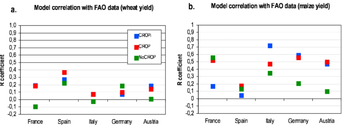
variations with those observed in the detrended FAO sta-tistical data for five European countries over the period 1972–2003. Figure 1 gives the correlation coefficients (R)
between yields resulting from all three simulation experi-ments (NoCROP, CROP, CROPi) and the FAO data for wheat and maize. The R coefficient is a useful measure of the model performance in terms of phase of simulated with observed interannual yield anomalies. SMI09a only dis-cusses the magnitude of these anomalies, relative to yield mean, using the coefficient of variation (CV, equals stan-dard deviation divided by mean) compared between model results and data.
3.1. Phasing and Correlation Between Time Series 3.1.1. Effect of Crop Parameterization and Irrigation
[23] On average, the R values are low, indicative of the
difficulty to reproduce the phase of year‐to‐year fluctuations in crop yield at large scale. This reflects uncertainties in agricultural practices, soil characteristics, climate drivers, and model structure and parameters. The model‐data cor-relation is always higher for maize (Figure 1b) than for wheat (Figure 1a) (except in Spain). This suggests that the parameterization of maize yield response to climate fluc-tuations is more realistic across Europe than the one of wheat.
[24] Despite the low R values, the CROP simulation
always outperforms NoCROP in the comparison with the FAO historical yield data (Figure 1), except for wheat in Germany. It is encouraging to see that the modified parameterization of crop types in ORCHIDEE via STICS brings an improvement in the simulation not only of phe-nology (“seasonal leaf cycle” section of SMI09a) but also of the interannual variability in productivity.
[25] This improvement in the phase of interannual yield
variations was not detectable in the CV values, representa-tive of variability amplitude [SMI09a]. For instance, for wheat in France, Spain and Italy, the CROP and NoCROP simulations give similar CV values but the phase is always more realistic in CROP. The same is true for wheat in Austria (better model‐data correlation using the CROP simulation results): even if the coupled model overestimates variability amplitude more than the standard version does, the phase is better captured in the CROP simulation. Figure 1. Correlation coefficients between yields reported in the FAO data and simulated by Standard ORCHIDEE (NoCROP: green), ORCHIDEE‐STICS nonirrigated (CROP: red) and irrigated (CROPi: blue) for (a) wheat and (b) maize for the five European countries over the 1972–2003 period.
[26] The effect of irrigation on the simulated interannual
variability of maize yield (comparison of CROPi with CROP; see Figure 1b), differs between regions. Irrigation improves the correlation between simulated and FAO yield time series in Italy, but it has the opposite effect in France. In Germany and Austria, where water availability in summertime is larger than in Italy, irrigation does not make much difference in the phasing of simulated and FAO time series. As expected, values for NoCROP are usually closer to those for CROP than to those for CROPi. Regarding the variability amplitude, accounting for non-irrigated crops decreases the value of the CV by ≈15%. Irrigation has the remarkable effect to decrease it again by ≈40% [SMI09a].
3.1.2. Simulated Versus Observed Yield Anomalies for the 1976 and 2003 Drought Years
[27] Figure 2 compares the maize yield time series between
the FAO annual statistics and our simulation results, both without irrigation (CROP) and with irrigation (CROPi). Sim-ulated and observed (detrended) yields are expressed as nor-malized anomalies, i.e., anomalies relative to their respective mean over 1972–2003, further divided by their standard deviation over the same period. These two countries, France and Italy, have been selected because they are the largest maize producers of EU‐25.
[28] ORCHIDEE coupled with STICS reproduces most of
the interannual climate‐driven maize yield fluctuations re-ported by the FAO. Especially, one can observe a large drop in yield in 1976 in France (Figure 2a) but not in Italy (Figure 2b). In contrast, the 2003 negative anomaly affects both countries. Such important geographic yield reduction
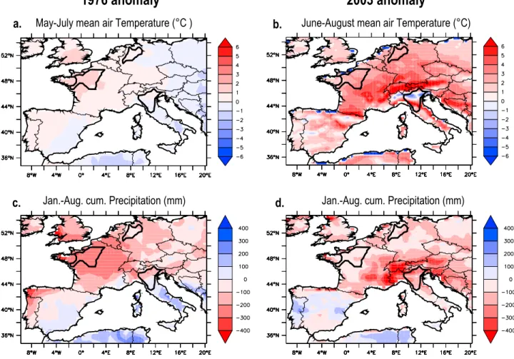
differences between 1976 and 2003 are well reproduced by the CROP and CROPi simulations. They can be explained by differences in the spatial pattern of the climate anomalies between both drought years. The center of action of the pronounced 1976 drought (Figures 3a and 3c) is located in the North and West of France (−400 mm cumulative January–August precipitation deficit), whereas the one of the 2003 drought and heat wave (locally also −400 mm cumulative January–August precipitation deficit, +6°C average June–August temperatures) is located over the alpine countries (southeastern France, northern Italy, southern Germany and Austria) (Figures 3b and 3d).
3.2. Regional Patterns of the 2003 Yield Loss Magnitude
[29] We now focus on the 2003 climate extreme and its
impact on crop yields. The choice of 2003 as a test year for the model is justified by (1) the widespread and extreme June–August heat conditions, (2) the interesting drought which started in spring and extended until the late summer, and (3) the abundance of data and modeling studies [Ciais et al., 2005; Granier et al., 2007; Reichstein et al., 2007; Vetter et al., 2007], yet without specific focus on the response of crops.
[30] Figure 4 shows how the regional pattern of the 2003
normalized anomaly (see definition in the previous section) of maize yield compares between the FAO data and the CROP or NoCROP simulation. The data (Figure 4a) indi-cate that maize yield in France, Italy, Germany and Austria was strongly affected by extreme temperatures and drought and suffered a yield loss as high as 4 times the standard deviation (−4s). In contrast, maize yield in Spain was not significantly reduced, as compared to mean values.
[31] The CROP simulation (Figure 4b) shows a similar
pattern of negative yield anomaly with maximum losses along a diagonal going from southwestern France to eastern Germany. The Po Valley in Italy experienced an average yield loss, yet with few grid cells showing a gain. The yield drop pattern is very well correlated with the 2003 summer temperature anomaly pattern (Figure 3b) with maxima around the Alps.
[32] The modeled maize yield loss in the CROP
simula-tion is in good agreement with country average values (diagnosed from FAO statistics), though slightly less dra-matic, locally reaching −3s only. In contrast, the yield anomaly shows a less realistic spatial distribution in the NoCROP simulation (Figure 4c). The C4“super grass” PFT (used by default to describe C4 crops in this reference simulation) seems to benefit from the abnormally warm temperatures in northeastern Europe in 2003. Consequently, the NoCROP simulation produces an unrealistic increase in NPP as well as in yields (positive anomaly) in Germany and Austria during the summer 2003, which is invalidated by the FAO data showing, on the contrary, a drastic drop in both countries.
3.3. Discussion
3.3.1. Evaluation of Model Performance
[33] The more realistic phase of interannual yield variations
simulated by ORCHIDEE‐STICS (nonirrigated) compared with the model version without crops (Figures 1a and 1b) Figure 2. Normalized yield ((Yield‐Mean)/Std.Dev.)
1972–2003 series simulated by ORCHIDEE‐STICS nonirri-gated (CROP: red) and irrinonirri-gated (CROPi: blue) compared with FAO data (black) for maize in (a) France and (b) Italy. The grey boxes indicate the 1976 and 2003 extreme events.
indicates that the productivity response to climate variability is improved when accounting for crop specificities (more realistic phenology). The fact that the values of the correlation coefficient (R) remain quite low for wheat (Figure 1a) can be due to a difference in the definition of wheat between model output and data: the simulated single winter wheat variety does not respond to climatic variability in the same way as the observed (FAO) wheat, which encompasses a number of winter‐ to spring‐type varieties along a gradient of needs for cold (vernalization) and warm (maturation) temperatures. Besides the heterogeneity of soils and agricultural practices mentioned in SMI09a (see the last three paragraphs before section 5), which is not accounted for in the modeling approach, the difference in the surface areas contributing to the aggregated country‐level yield (see Table 2 in SMI09a) is also a cause for the discrepancy between simulated and observed interannual variability. In the case of maize (Figure 1b), we model only grain maize and not silage maize. Irrigation can reverse the response to a climate anomaly by letting crops take advantage of warmer tem-peratures and relieving water limitation (Figures 2a and 2b). Depending on the country considered, the data are better correlated with the simulation with irrigation (Italy) or without (France). Using a realistic fraction of irrigated crops
would combine the two possibilities and improve the final correlation in both countries.
[34] Absolute yield anomalies [Smith, 2008] simulated for
maize by ORCHIDEE‐STICS in 2003 in France, Germany and Austria (CROP simulation) are equivalent in amplitude to those reported in the FAO data. On the other hand, the standard deviation is about twice as large as observed. This is because the model simulates yield accidents that do not appear in the FAO data (e.g., 1983 and 1994 in France); this suggests that the sensitivity of ORCHIDEE‐STICS forced by homogeneous agricultural practices is overestimated. Therefore the intensity (anomaly divided by Std. Dev.) of the yield response to the 2003 extreme event is under-estimated in the model (Figures 4a and 4c).
[35] The performance of ORCHIDEE‐STICS for 2003
still remains much better than that of ORCHIDEE without crops, the latter showing a too low NPP reduction and even a NPP increase over northeastern regions (Figure 4b). The intensity of the yield drop of irrigated maize in 2003 [Smith, 2008] is locally as high as reported in the FAO data, because of a lower standard deviation of irrigated versus nonirrigated maize. This response suggests that irrigation cannot prevent maize from all damages and reminds that the 2003 summer was characterized by extreme temperatures and not only by drought.
Figure 3. Mean ambient air temperature (May–July or June–August, °C) and cumulative precipitation (January–August, mm) forcing anomalies (relative to the 1972–2003 mean) in the contrasted years (a and c) 1976 and (b and d) 2003.
3.3.2. Investigating Mechanisms of the Crop Productivity Drop
[36] After evaluating its overall ability to reproduce
data, the model is used to study causes of the productivity drop. These can be, for instance, changes in the seasonal leaf cycle, transpiration, photosynthesis and/or autotrophic respiration.
3.3.2.1. Water‐Use Efficiency
[37] Irrigation was found to have more effect mitigating
maize yield drop in France in 1976 than in 2003 [Smith,
2008]. This is also visible in Figure 2a, where the 1976 yield anomaly in CROPi is close to zero. Rain‐fed maize yield drop in CROP in 1976 was mainly due to drought stress, relieved when irrigation is applied. Note that irriga-tion amount has no upper limit in the model whereas it has in reality during severe droughts, because of competing water uses beyond agriculture. This yield anomaly ampli-fying effect is not accounted for in the model. Water‐Use Efficiency (WUE, defined as annual GPP or NPP divided by annual transpiration) by rain‐fed maize was reduced in CROP in both extreme years: transpiration decreased less than GPP and NPP did relative to a mean year, so less CO2
was assimilated per unit water transpired. However, irriga-tion in 1976, increasing WUE by≈+2 gC/m2/mm, restored near‐to‐normal WUE levels, whereas it could not mitigate the part of the WUE reduction due to thermal stress in 2003.
[38] We found that WUE was much reduced in 2003, not
only for maize in France and Italy, but also for winter wheat and soybean, and in Germany (by ≈−1 to −3 gC/m2/mm). Nevertheless, winter wheat suffers less as its phenology allows it to escape part of the high summer temperatures. Escape is one of the three drought adaptation mechanisms, the others being avoidance (deeper rooting and stomatal closure) and tolerance or resistance (osmotic adjustments) [Fageria, 1992]. Based on the GPP measured on trees at several FluxNet sites in 2003, Reichstein et al. [2007] in-terpreted water stress to be the main cause of tree produc-tivity drop. They found that the WUE of forest vegetation, unlike that of agricultural vegetation, was only very slightly reduced in 2003 compared with 2002. This WUE reduction was smaller than the difference between forest sites. Com-paring ORCHIDEE‐STICS results with cropland site eddy‐ covariance measurements would allow us to identify whether the interpretation differences are due to (1) potential biases in the model and/or flux data or to (2) real differences in the response of crop versus forest ecosystems to the 2003 heat wave.
3.3.2.2. Seasonal Leaf Cycle
[39] The absolute reduction of carbon and water fluxes
simulated by ORCHIDEE‐STICS for crops in both 1976 and 2003 extreme years is primarily due to a lower maximum LAI and a shorter effective growing season duration [Smith, 2008]. An overall vegetation productivity drop linked to the growing season shortening was indirectly observed by sat-ellite in 2003. The MODIS faPAR data show a clear reduction in vegetation photosynthetic activity in western Europe from July to September (following the June to August climate anomaly) relative to the 2000–2004 mean [Reichstein et al., 2007]. As in ORCHIDEE‐STICS simulation results, ecosystems in Spain are unaffected by the 2003 climate anomaly. Reichstein et al. [2007] found that the observed faPAR negative anomaly over July–September in western Europe was 5 times larger than the standard deviation cal-culated on the MODIS (2000–2004) and AVHRR‐GIMMS (1982–2002) time series. This highlights the significance of the vegetation productivity drop due to the extreme 2003 summer.
3.3.2.3. Autotrophic Respiration
[40] In our simulations, the decoupling of CO2and H2O
fluxes at the stomata level was strong in 2003, due to higher than optimal temperatures for photosynthesis. In addition, Figure 4. Intensity (normalized yields over 1972–2003) of
2003 extreme maize yield drop reported in the (a) FAO data compared with that simulated by (b) ORCHIDEE‐STICS (CROP) and (c) Standard ORCHIDEE (NoCROP) for each European grid cell comprising more than 25% agriculture.
the simulated autotrophic (maintenance and growth) respi-ration CO2flux was found to decrease by≈30% in August
2003 in Italy relative to a mean year because of the reduced crop biomass and growth. But autotrophic respiration actu-ally increased at the ecosystem level relative to GPP which experienced a ≈50% reduction at the same time. Mainte-nance respiration is not only controlled by standing active biomass but also by temperature, extremely high in August 2003. NPP equals GPP from which autotrophic respiration has been deducted. The NPP to GPP ratio of rain‐fed and irrigated maize is of ≈35–50% and ≈50–55%, respectively, during“normal” years in the model. This ratio was reduced down to ≈25–45% and ≈45–50%, respectively, in 2003 in all studied countries in both ORCHIDEE‐STICS simula-tions [Smith, 2008].
4.
Results: 2003 Anomalous European Carbon
Source
[41] We now analyze how croplands contributed to the
large positive carbon flux anomaly observed over Europe in 2003, due to a drought coupled with extreme summer temperatures. The net carbon flux exchanged between the atmosphere and the biosphere, NEE, is expressed so that negative values indicate a biosphere sink and positive values a source to the atmosphere. On fine spatial scales, we used ORCHIDEE‐STICS to quantify NEE anomalies. On coarse spatial scales, we used independent atmospheric inversions relying upon CO2concentration gradients (see section 2.2)
and atmospheric transport models.
4.1. Enabling the Comparison Between Ecosystem Model Fluxes and Large‐Scale Atmospheric Inverse Estimates
[42] Inversion results are used in this study to cross‐
validate NEE estimates provided by ORCHIDEE‐STICS on the continental scale. In ORCHIDEE and ORCHIDEE‐ STICS, NEE is computed as the difference between NPP and soil heterotrophic respiration (HR). NPP, calculated sepa-rately for each natural or agricultural vegetation type, is averaged and weighted by the relative fractional area of each PFT in each grid cell. HR is computed in each grid cell by lumping together CO2emissions from the litter as well as soil
carbon pools of all vegetation types. For cultivated vegeta-tion, these decomposing carbon pools receive input only from nonharvested NPP (crop residues), the harvest being exported away from the ecosystem and ignored on the grid cell scale. Crop fields are not tilled in our simulations. On a European scale, we have to account for harvested agricultural products being consumed by humans and animals, releasing CO2back
to the atmosphere. To do so, we assume the crop harvest to be respired within 1 year, that is 1/365 of the harvest returns to the atmosphere each day. Adding this source (positive flux) to the simulated NEE, in order to close the continental carbon balance, makes“bottom‐up” model estimates (ORCHIDEE and ORCHIDEE‐STICS) consistently comparable with “top‐ down” land fluxes (PEY08 and ROE03 inversions). To fur-ther enable this comparison, inversion and ecosystem model estimates of NEE (computed at different spatial and temporal resolutions) were aggregated over the same European domain (−10° to 20° east and 35° to 55° north) and a 6 month period around the summer (May–October).
[43] In section 4.2, we compare the modeled seasonal
variation of European NEE between the averaged 1996–2002 period and the 2003 abnormal year. In order to interpret the results independently from model incomplete spin‐up simulations (i.e., carbon pools were initialized to values not exactly corresponding to equilibrium), the NEE values shown include a normalization. Assuming that ecosystem‐ atmosphere carbon exchanges tend toward zero on a long time period, we subtracted the 1996–2002 annual mean NEE value both from the 1996–2002 average and 2003 extreme seasonal cycles. This normalization was done independently for each simulation (CROP, CROPi and NoCROP), for each natural and agricultural vegetation and in each grid cell.
[44] In section 4.3, we show the spatial distribution of the
2003 NEE anomaly (difference between 2003 and 1996– 2002) summed over May to October. Finally, section 4.4 compares European NEE anomalies over 1996–2003 between the three bottom‐up simulations (CROP, CROPi and NoCROP) and two inverse model results (PEY08 and ROE03).
4.2. Seasonal Development of the 2003 NEE Anomaly 4.2.1. With and Without Crop Modeling
[45] The typical seasonal variation of NEE in Europe
[Vetter et al., 2007] is characterized by (1) a net CO2uptake
due to the growing plants and by (2) a net CO2release the
rest of the year while plants are dead, dormant or little productive (at the beginning and end of the growing sea-son) and soil microbial activity dominating the flux. This seasonal structure can be seen in both 1996–2002 mean and 2003 extreme years in all three ORCHIDEE‐based simulation results in Figure 5a. Note that these results were computed for combined natural and agricultural vegetation (resp. 60% and 40% of Europe’s vegetated surface area [Ramankutty and Foley, 1999]). Two main features appear from the results of all simulations: in 2003 the spring maximum carbon uptake was reduced, and the end of the Carbon Uptake Period (CUP, defined as the period with negative NEE) occurred about 1 to 1.5 months earlier than on average during 1996–2002.
4.2.1.1. Spring Season
[46] Even though the year 2003 was an absolute record for
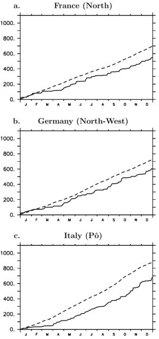
its elevated temperatures from June to August [Schär and Jendritzky, 2004], the divergence between the 2003 and the mean NEE (plain and dashed lines, respectively) already appeared at the end of April. The early NEE source anomaly (Figure 5b) hence started developing in the spring, i.e., much earlier than the summer heat wave, in all three simu-lations (CROPi, CROP and NoCROP). It can be explained by an early drought signal resulting from a precipitation deficit at the beginning of year 2003 and causing water stress limita-tions on vegetation productivity. This precipitation deficit is already noticeable in March in France (Figure 6a) and Ger-many (Figure 6b) and even in February in Italy (Figure 6c). The amplitude of the spring carbon uptake was consequently reduced, as compared to the reference period (Figure 5a): for instance, the daily European mean NEE in May 2003 equals −5 TgC/d (or even −4 TgC/d in NoCROP) instead of −6.5 TgC/d during 1996–2002 in all three simulations. Once started in the spring, the NEE source anomaly of year 2003 further developed and increased in the summer (Figure 5b).
4.2.1.2. Summer Season
[47] The simulated NEE (Figure 5a) shows a rather similar
structure between CROP and CROPi during the anomalous year 2003 (as well as during the mean year), apart from the expected irrigation effect allowing a larger carbon uptake (blue lines). In contrast, the NEE seasonal cycle is quite
different between CROP (or CROPi) and NOCROP during 2003 (as well as during the mean year). The same differ-ences can be noticed in Figure 5b.
[48] During the mean year (dashed line in Figure 5a), the
slowing down of the carbon uptake after the maximum assimilation phase in May is regular in NoCROP whereas Figure 5. Seasonal cycle of NEE summed over Europe (TgC/d) for the ORCHIDEE‐based experiments
NoCROP (green lines), CROP (red lines) and CROPi (blue lines). (a) Normalized values (Normalized European NEE) for the year 2003 (plain lines) versus the 1996–2002 mean (dashed lines). (b) The 2003 European NEE anomalies. For ORCHIDEE and ORCHIDEE‐STICS NEE, we accounted for smaller contributing surface areas along the coast and nonvegetated areas such as glaciers in the Alps.
the CROP (and CROPi) results show a secondary NEE peak in August. In 2003, the simulated responses in CROP and NoCROP are even more different from one another (compare green and red plain lines in Figure 5a). Without an explicit crop parameterization, the simulated NEE (NoCROP) is more sensitive to hot conditions in summer 2003. From June on, the NEE anomaly in NoCROP is thus larger than the one in both CROP and CROPi simulations (Figure 5b). Back‐to‐normal NEE values are simulated by October in both CROP and CROPi experiments and only by December in NoCROP (Figures 5a and 5b).
4.2.2. Specific Crop Phenology and Irrigation Effects [49] We now analyze, inside the two ORCHIDEE‐STICS
simulations, the response of the different crop PFT and the effect of irrigation in normal and 2003 extreme conditions. 4.2.2.1. Phenology Effect
[50] In the CROP and CROPi simulations during normal
years, there is a characteristic secondary peak in NEE during August (Figure 5a). This peak is explained by the intense growth of the spring crops maize and soybean (representing PFT C4 and spring‐type C3, respectively) increasing carbon uptake. Their maximum uptake phase occurs after the winter crops have been harvested generally in July. Harvest of spring crops is delayed to October. The two‐peak structure is not at all present in the NoCROP simulation as mentioned in the previous section. During 2003 in CROP and CROPi, the August NEE peak was suppressed (Figure 5a). This behavior is principally due to the fact that maize and soy-bean growth is negatively impacted by the hot August temperatures, which are higher than the parameterized optimum temperatures for photosynthetic enzymatic activity in the model (see Table 1 in SMI09a). Note that the crop phenological signal in the aggregated CROP and CROPi mean NEE, and the crop response to the 2003 climate anomaly, are visible although agricultural PFT cover only ≈40% of our European domain.
[51] Due to the reduced net carbon uptake amount and
duration in 2003 relative to the normal two‐phase CO2
assimilation (Figure 5a), CROP and CROPi curves of the NEE anomaly also show a pronounced two‐peak structure (Figure 5b). The second anomalous source to the atmo-sphere is related to the cancelation in 2003 of the usual August secondary peak in the carbon uptake in CROP and CROPi. As a result, ORCHIDEE‐STICS produces two ano-malies, in June (≈+3 TgC/d) and in August (≈+1.5 TgC/d), whereas ORCHIDEE without crops simulates a persistent anomalous source from June to August (≈+3 TgC/d) slowly decreasing after this date. Integrated over the 6 months from May to October the European carbon source anomaly is nearly twice as large in NoCROP (+0.41 GtC) than in CROP (+0.25 GtC) (Table 1). The two peaks that can be seen in the NoCROP results reflect the effect of varying temperature extremes inside the overall heat wave (Figure 5b). There is no link here with winter‐ and spring‐type phenologies as in the CROP and CROPi simulations. However this effect of varying temperature anomalies applies to all simulations and
Table 1. Decomposition of the 2003 NEE Anomaly Into Its Fluxes and Contributions From Vegetation Types in the Three ORCHIDEE‐Based Simulationsa
May–October European CO2Flux (GtC) NoCROP CROP CROPi
NEE on average (1996–2002) −0.20 −0.20 −0.26 NEE in 2003 +0.21 +0.05 −0.06 DNEE +0.41 +0.25 +0.20 DHR +0.06 −0.04 ≈0 −DNPP +0.35 +0.29 +0.20 DNPPnaturalPFT −0.09 −0.09 −0.06 DNPPagriculturalPFTb −0.26 −0.20 −0.14 a
Negative numbers indicate a sink, and positive ones indicate a source of CO2to the atmosphere.
b
In the model vegetation map, agricultural vegetation covers≈40% of the European domain and natural vegetation≈60%.
Figure 6. Daily cumulative precipitation (mm) from the climate forcing fields in 2003 (plain line) and averaged over 1972–2003 (dashed line), in highly agricultural regions of (a) France (north), (b) Germany (northwest) and (c) Italy (Po).
exacerbates the two‐peak structure of the CROP and CROPi NEE anomalies.
4.2.2.2. Irrigation Effect
[52] The effect of irrigation is deduced by comparing
CROP (red lines) and CROPi (blue lines) simulation results (Figure 5a). In normal conditions (dashed lines), irrigation starts impacting on cropland CO2 uptake in June, when
spring crops like maize are in their exponential growth phase. In 2003 (plain lines), the onset of irrigation calculated by the STICS model occurs 2 months earlier (already during
the early drought in April). In addition, the total irrigation amount was≈200 mm larger than during a mean year, for maize cultivated in the areas most affected by the climate anomaly. In all cases, irrigation stops at spring crop harvest and has apparently no lagged effect on soil respiration thereafter. In normal conditions, net carbon uptake is found to be enhanced by irrigation (+30% over May–October in Europe; see Table 1). This signal in NEE is explained by a +17% NPP increase dominating over a +14% soil respira-tion increase [Smith, 2008]. In 2003, the European NEE simulated in CROP over May–October turns out to be a slight carbon source (+0.05 GtC) rather than an uptake (−0.06 GtC; see Table 1). This is due to the crop produc-tivity drop (though smaller than the supergrass producproduc-tivity drop in NoCROP). Irrigation of crops allows European ecosystems altogether (natural and agricultural vegetation in CROPi) to keep behaving as a small carbon sink over May– October (Table 1).
4.2.2.3. Summary
[53] In summary, irrigated crops absorb more CO2 than
rain‐fed ones, in normal years as well as in 2003. However, this amelioration of uptake is relatively more important in 2003. Turned in another way, the 2003 heat wave reduces CO2uptake and hence generates a source anomaly in both
simulations, but in a smaller proportion when irrigation is turned on (Figure 5b). Overall, Figure 5b shows that irri-gation reduces the negative impacts of heat waves and drought on NEE, thus decreasing the 2003 May–October European carbon source anomaly by−17%, as compared to the CROP simulation ignoring irrigation. Despite irrigation mitigating the productivity drop in 2003, the NEE anomaly is found to be temporarily larger in the simulation with irrigation than in the one without only in late July and early August (Figure 5b).
[54] It is interesting to see that although irrigation is
applied mainly to maize (representing up to ≈25% of total European vegetated area in local French and Italian maize producing regions and less than ≈5% elsewhere), this practice has a sufficiently strong impact on the modeled aggregated NPP at continental scale to be detected in the total European NEE and NEE anomaly curves. Beyond this irrigation effect, introducing crops in ORCHIDEE‐STICS changes significantly the seasonal phase and amplitude of the NEE anomaly in 2003. The specific parameterization of winter‐ and spring‐type crop phenology acts to attenuate the 2003 carbon loss to the atmosphere, via a smaller source to the atmosphere in July–October.
4.3. Spatial Pattern of the 2003 NEE Anomaly [55] The spatial pattern of the May to October NEE
anomaly in 2003 (Figures 7a–7c) clearly reflects the area of maximum heat and drought, centered on alpine countries (Figure 3). The source anomaly is more pronounced and more widespread over northeastern Europe in NoCROP (up to +600 gC/m2; see Figure 7a) as compared to CROP (Figure 7b). The growing season length is potentially shorter (late spring until early autumn) in the northeast compared with the south. The higher sensitivity of the NoCROP fluxes in this region is explained by the fact that the“supergrass” PFT has its growth peak later in summer in the north: it is thus more exposed to midsummer stress in 2003 without much compensation possibilities (Figure 7a). In comparison, Figure 7. Spatial pattern of the 2003 “summer” (summed
from May to October) NEE anomaly (gC/m2, relative to the 1996–2002 mean) for the ORCHIDEE‐based experi-ments: (a) NoCROP, (b) CROP and (c) CROPi.
in ORCHIDEE‐STICS, the winter crops are in their maxi-mum growth phase in late spring, drying in June and har-vested in July, hence escaping from midsummer stress (Figure 7b).
[56] In northwestern Germany and east Czech Republic,
ORCHIDEE‐STICS winter crops are even found to be more productive in May–October 2003 than under normal con-ditions, because of warmer spring temperatures and suffi-cient water availability. This locally positive impact of the climate anomaly causes a sink anomaly (up to−300 gC/m2; see green areas in Figure 7b). Additionally, irrigation en-hances carbon uptake of spring‐type C3 crops in Poland. This is why the northern half of this country shows in 2003 a large anomalous net carbon sink in CROPi (−300 gC/m2
; see Figure 7c) compared with a small anomalous source in CROP (+150 gC/m2; see Figure 7b).
[57] In Croatia, Hungary and Serbia, where maize
culti-vation predominates (C4 crop, irrigated or not) (FAO ProdStat data, 2007, available at http://faostat.fao.org/site/ 567/default.aspx), we simulate an anomalous source of CO2
to the atmosphere during 2003 in all three experiments (Figures 7a–7c). This robust result is consistent with the exceptional maize yield drop simulated and observed in 2003 (Figure 4c). In contrast, except in the Balkan region, the total NEE anomalous signal in 2003 is controlled by the response of the C3 crops, which dominate agricultural land cover.
4.4. Comparison With Inversion Results 4.4.1. Error and Scale Issues
[58] Inversions do not give evidence for a two‐peak
sea-sonal structure in total European NEE and NEE anomaly (not shown), unlike our simulations with crops discussed in section 4.2.2. This is likely because inversions make use either of monthly atmospheric CO2observations as PEY08
[see Piao et al., 2009] or of smooth temporal regularization constraints as ROE03 [Rödenbeck et al., 2003]. However, an anomalous CO2source in 2003 is well detected in both
inversions. The amplitude and duration of this inverse source [Smith, 2008] is similar to those simulated by ORCHIDEE‐STICS (CROP and CROPi) but smaller than those simulated by ORCHIDEE without crops (Figure 5b). Because errors associated with the inverse estimates remain rather large on a monthly time step [Gurney et al., 2005], we will not discuss in the following the exact timing of the inverse anomalies but only the averaged value over 6 months (May–October).
[59] Although both inversions infer an anomalous carbon
source in 2003 over Europe, the spatial patterns of this flux anomaly (not shown [Smith, 2008]) are not straightforward to interpret. The center of the May–October NEE anomaly is located in eastern Europe in the PEY08 inversion, against northwestern Europe in the ROE03 inversion. Given the rather coarse spatial resolution of both inversions (i.e., the grid resolution of the transport models, roughly 2° × 3°) and their reliance on a priori settings (e.g., prior flux pattern and associated error structure; see section 2.2), their results cannot be safely interpreted on a fine spatial scale. Large differences appear between both inversions in individual grid cells (up to 300 gC/m2over May to October), which are of larger magnitude than the differences between the
ORCHIDEE‐based simulations (Figures 7a and 7b). These regional differences reflect partly random noises and partly biases of the inversions. The inverse flux regional patterns have to be discussed together with the posterior flux un-certainties estimated by the inverse procedure. Such an analysis is beyond the scope of this paper.
4.4.2. 2003 Anomalous Carbon Source Quantification Over Europe
[60] When looking at the above‐mentioned differences
between inversion fluxes (for individual grid cells and time steps) and summing up their absolute values, we find that this sum is 3 times larger than that of the differences between bottom‐up simulated fluxes [Smith, 2008]. Inver-sion largely suffer from too scarce atmospheric observation. On this fine spatial and temporal scale, refining the process‐ based bottom‐up modeling approach appears to be a more promising way to reduce uncertainties in the carbon cycle before significant improvements can be achieved to increase the resolution of regional inverse estimates.
[61] However, on an integrated European and 6 month
scale, the difference between inverse estimates of the 2003 NEE anomaly (PEY08‐ROE03) is 3 times smaller than the difference between bottom‐up estimates (CROPi‐NoCROP). This result reflects that inversion flux anomalies are more robust than mean fluxes and that aggregated fluxes are less uncertain [Carouge et al., 2010]. It further suggests that the information content of inversions is high enough to be able to falsify the ecosystem model parameterizations.
[62] From May to October, terrestrial ecosystems were an
anomalous CO2 source in Europe in 2003 relative to the
1996–2003 period (Figure 8), as demonstrated by the three ORCHIDEE‐based simulations as well as by the two in-versions (CarboEurope reports; see http://www.carboeurope. org/). In addition, 2003 is the only year for which bottom‐up and top‐down estimates consistently indicate a NEE anom-aly of the same sign. At face value, during“normal” years the interannual variability is poorly correlated between inver-sions and poorly correlated between any inversion and any ORCHIDEE simulation. In 2003, ORCHIDEE without crops gives an anomalous source of +0.41 GtC, nearly twice as large as the +0.20–0.25 GtC anomaly simulated by both inversions. ORCHIDEE‐STICS produces a 2003 anomalous loss of carbon of +0.25 GtC and +0.20 GtC for nonirrigated and irrigated crops, respectively. Therefore, for an extreme climate event like in 2003, both inverse anomalies agree better with the ecosystem model result when crop para-meterizations are included (Figure 8).
4.5. Discussion
4.5.1. Relating 2003 European NEE Anomaly and Crop Productivity Drop
[63] In order to better understand the temporal
develop-ment and spatial pattern of the 2003 carbon flux anomaly, we have decomposed the total European NEE from each simulation into its components, such as NPP and HR of opposite sign, or contribution from natural and agricultural vegetation to the aggregated value (Table 1) [Smith, 2008]. 4.5.1.1. Role of NPP Versus Soil Respiration
[64] The main cause for the 2003 abnormal loss of CO2
from European ecosystems is clearly a drop in NPP, induced by a combination of thermal and drought stress affecting
plant Radiation‐Use Efficiency (RUE). This effect is domi-nant over the small reduction of HR due to drier soil con-ditions and lower input to the litter carbon pool. For instance, in the CROP simulation, the NPP drop explains≈90% of the +0.25 GtC NEE source anomaly and≈100% or 85% of the respective corresponding anomalies in CROPi and NoCROP (Table 1). Thanks to an intercomparison study between biosphere models, Vetter et al. [2007] also showed that respiration processes (vegetation and soils) were less affected than photosynthesis by the heat wave. We found that irri-gation tends to increase soil respiration in 2003, by relieving water limitations on the modeled Soil Organic Matter (SOM) decomposition rate, which is then enhanced by warmer temperatures. However, irrigation mitigates the NPP drop more than it favors respiration, thereby reducing the mag-nitude of the NEE source anomaly compared with nonirri-gated simulations.
4.5.1.2. Role of Crop Versus Natural Vegetation [65] Crops were more sensitive than natural vegetation to
the heat wave: as simulated by ORCHIDEE‐STICS in the CROP experiment, the NPP drop of European crops over May–October was as dramatic as −40%, against −12% for natural vegetation. Although crops cover only≈40% of the European domain, their response explains ≈70% of the anomalous NPP drop in 2003 and hence≈60% of the Euro-pean NEE source anomaly (Table 1). This big signal illustrates the influence that cropland ecosystems (specific phenology and productivity) have on larger‐scale CO2fluxes, in response
to an extreme event such as summer 2003 in Europe. 4.5.2. Improved Model Results and Implications for the Carbon Cycle
[66] Looking at the response of individual agricultural
PFT allows us to explain the differences between the results of the three model versions. The fact that the 2003 NEE anomaly is smaller in the CROP and CROPi simulations
than in the NoCROP one (Figures 8, 5b, and Table 1) is explained by the specific winter‐type phenology (winter wheat) introduced in the ORCHIDEE model via STICS, to represent part of the C3 crops. This vegetation type achieves most of its growth during the spring and is harvested at the end of June or in July, which minimizes exposure to mid-summer stress conditions. In ORCHIDEE‐STICS after July, only part of the C3 crops, the spring‐type C3 crops (soy-bean), are responsive to the hot temperature anomaly in 2003 (Figure 7b). They share the surface area allocated to C3 agricultural vegetation in each grid cell with the already harvested winter crops, which experience no NPP change in the second half of the year. In NoCROP, these two pheno-logical types are not distinguished but represented by a unique generic C3“supergrass”, growing mainly in summer and not subject to harvest, an agricultural practice not ac-counted for in ORCHIDEE without STICS. The “super-grass” suffers in 2003 from early senescence, particularly in the northeast of Europe (Figure 7a). NPP collapsed to almost zero values by mid‐August, leaving heterotrophic respiration as the dominant process controlling NEE after that date (Figure 5a). Similar results were obtained by Ciais et al. [2005]. The average NoCROP NPP over 1996–2002 is controlled by a longer growing season, with grass produc-tivity being even maintained to a nonzero level during the winter [Smith, 2008]. This poor representation of specific crop phenology amplifies the 2003 NEE response by the initial model version.
[67] The main irrigation effect in 2003 was found to be the
mitigation of the NPP drop. However, following winter crop harvest, increased HR sustained by wetter soils in CROPi induces a temporary higher anomalous CO2 source to the
atmosphere than in CROP. This soil respiration enhance-ment by irrigation (effect also found, for instance, by Verma et al. [2005]) is shortly, in late July and early August 2003, Figure 8. Cumulative May to October European NEE anomalies (GtC) compared over the 1996–2003
period between ORCHIDEE‐based simulations NoCROP (green line), CROP (red line), CROPi (blue line) and the two inversion estimates PEY08 (black line) and ROE03 (grey line). For ORCHIDEE and ORCHIDEE‐STICS NEE, we accounted for smaller contributing surface areas along the coast and non-vegetated areas such as glaciers in the Alps. For Inverse NEE only a land‐sea mask at coarser resolution applies.
dominant (Figure 5b) over the NPP decrease of the newly growing spring crops (C3 and C4).
[68] The NEE responses to the climate anomaly in the
three model versions also include the contribution of C4 crops. In the CROP simulation, maize is impacted in a similar way to the spring‐type C3 crops (soybean) and suffers from a productivity drop. In NoCROP, unlike the C3 “supergrass”, the C4 “supergrass” grows better in 2003 in northeastern Europe. Its growth, favored by near‐optimum summer temperatures for C4 photosynthesis as parameter-ized for tropical C4 crops in ORCHIDEE (see Table 1 in SMI09a), locally causes a CO2sink anomaly. Yet, this sink
anomaly occurring in areas where the CO2flux anomaly is
controlled by C3 crops does not appear in the NoCROP NEE anomaly aggregated over vegetation types (Figure 7a). [69] The drop in the observed (FAO) and simulated
(CROP) maize yields was analyzed in the first result part of this paper (section 3) and the unrealistic NoCROP results already highlighted. Note that results from sections 3 and 4 are not directly comparable. Nevertheless, though the reference periods in both studies are different, the means and anomalies in climate forcing variables and simulated NPP are similar (3 to 5% discrepancy in resp. CROPi et CROP mean NPP) between 1972–2003 and 1996–2002, respectively, chosen to take advantage of the observed data. In addition, the May to October months considered for the temporal integration include the most part of the crop growing season and the abnormally dry and hot summer months in 2003. This 6 month period is a good proxy for the response over the year; even shorter periods were used in other studies [Ciais et al., 2005; Vetter et al., 2007].
[70] Overall, the simulation without crops produces an
unrealistically large May to October European net carbon uptake reduction in 2003 compared with simulations accounting for crops (Figure 8 and Table 1). Such an anomaly amounts to +0.41 GtC calculated over 6 months. Based on a model without a realistic representation of croplands, Ciais et al. [2005] estimated a +0.50 GtC anomalous source in 2003. Both estimates are comparable (taking into account differences in the simulation set‐up) and should be considered as overestimated. On the conti-nental scale, the two inversions converge to infer the much lower source of +0.20–0.25 GtC, also simulated by ORCHIDEE‐STICS with or without irrigation. Although we cannot exclude possible aliasing effects between the con-sidered European domain and the surrounding regions, it is very likely that inversions carry substantial information on this scale to improve the direct modeling of NEE. Accounting for crops in a vegetation model thus appears essential to bring the process‐based NEE estimates in line with inversion results (Figure 8). Though less dramatic than previously estimated, the 0.20–0.25 GtC anomalous CO2
source in 2003 increases by nearly a quarter the annual fossil fuel emissions across the domain (1.05 GtC/yr). This source also cancels the benefit of 2 years of the European bio-spheric sink estimated by Janssens et al. [2003].
5.
Conclusion and Outlook
[71] The main outcome of this work is the overall
improvement of simulation realism compared with the previous model version without crops, confirmed by the
confrontation of model results against several data or complementary estimates on various temporal and spatial scales. This improvement in reproducing European cropland functioning in ORCHIDEE was mainly achieved by (1) the use of the winter‐type phenology coming from the STICS generic crop model; and (2) the inclusion of irrigation applied to summer crops.
[72] Further than just enhancing the agreement with
observed data for the seasonal cycle of LAI available for light interception, the coupled ORCHIDEE‐STICS model has shown a good ability to better reproduce agricultural yield mean [SMI09a] and variability at national level as well as carbon balance on a European scale. When accounting for crops in the model:
[73] 1. The estimation of crop yields with ORCHIDEE‐
STICS shows that the interannual yield anomalies, and their intensity in extreme years such as 2003, are better correlated with FAO records.
[74] 2. The 2003 European‐wide May to October NEE
anomaly is reduced, which brings the bottom‐up C loss in good agreement with inversion model estimates, considered as reliable on this scale.
[75] Given that ORCHIDEE was originally unable to
represent the specific phenology of cultivated plants and that STICS was initially not designed for geospatial applications, we can consider ORCHIDEE‐STICS as a satisfactory tool. These results demonstrate potential regional and interannual simulation improvement when associating two complemen-tary models with regard to the performance of each model alone on the intermediate scale considered.
[76] The choices made for yield derivation from NPP have
shown to be convenient for first‐order diagnostic analysis, as by Ciais et al. [2005] and comparison with FAO data. However, (1) refining based on STICS run with spatialized technical input, (2) including in ORCHIDEE‐STICS a specific carbon allocation scheme to plant organs such as grains for crops, and (3) considering a better model for respiration of harvested products would produce more reli-able estimates of the outgoing flux for European carbon cycle investigation. In LPJmL an intermediate carbon allo-cation scheme was developed, based on a daily alloallo-cation of the NPP according to the demand from the different plant carbon pools that is prescribed by functions derived from the SWAT model [Bondeau et al., 2007].
[77] Multimodel intercomparisons or model simulations
driven by a range of forcing data sets would allow high-lighting some model biases and uncertainties. Uncertainty reduction in agricultural statistics would be valuable, as well as in the atmospheric inverse approach.
[78] The inversion approach provides information on the
carbon cycle modeling on large spatial and temporal scales that is complementary to the process‐based approach. Inte-grating such large‐scale information into ORCHIDEE within a Carbon Cycle Data Assimilation System (CCDAS) [Rayner et al., 2005] is a promising way to improve our knowledge of the carbon cycle.
[79] Possible further strategies for validating terrestrial
ecosystem models such as ORCHIDEE‐STICS would include looking at variables of the hydrological cycle. Evapotranspi-ration is coupled with the carbon cycle via photosynthesis, and so is the surface and subsurface runoff, indirectly. A com-parison of variations in the simulated flux of water out of the
system with that observed in stream flow of European rivers could reveal not yet identified model biases and improvement targets. The upscaling of eddy‐covariance data and extension with time of the measurements over croplands started more recently than that over forests now offers a valuable network for water, energy and CO2flux validation.
[80] The coupled model outputs can potentially affect
further land‐surface related energetic processes influencing atmospheric circulation. Their effect could be analyzed within the framework of the IPSL coupled climate model sensitivity experiments.
[81] Feedbacks between climate change and land
affec-tation driven by economic and vegeaffec-tation productivity changes are already under investigation.
[82] Acknowledgments. Computational facilities were provided by CEA. Research and mobility were supported by CEA, INRA, CNRS, the AUTREMENT French ANR Project, EGIDE, Gilles Ramstein, Pierre Friedlingstein and Andrew Friend. We are very thankful to Christian Rödenbeck (MPI, Jena, Germany) for providing atmospheric inversion results and related valuable information. We acknowledge constructive interaction with Bernard Seguin (INRA, Avignon, France). We also thank Alexis Berg for useful comments on the manuscript and Edouard Davin for fruitful discussions. Finally, we are very grateful to both anonymous reviewers and the Associate Editor for substantial help in manuscript improvement.
References
Baker, D. F., et al. (2006), TransCom 3 inversion intercomparison: Impact of transport model errors on the interannual variability of regional CO2
fluxes, 1988–2003, Global Biogeochem. Cycles, 20, GB1002, doi:10.1029/2004GB002439.
Bondeau, A., et al. (2007), Modelling the role of agriculture for the 20th century global terrestrial carbon balance, Global Change Biol., 13(3), 679–706.
Bousquet, P., P. Peylin, P. Ciais, C. Le Quéré, P. Friedlingstein, and P. P. Tans (2000), Regional changes in carbon dioxide fluxes of land and oceans since 1980, Science, 290(5495), 1342–1346.
Brisson, N., et al. (2003), An overview of the crop model STICS, Eur. J. Agron., 18(3–4), 309–332.
Carouge, C., P. Bousquet, P. Peylin, P. J. Rayner, and P. Ciais (2010), What can we learn from European continuous atmospheric CO2
measure-ments to quantify regional fluxes, Part 1: Potential of the 2001 network, Atmos. Chem. Phys., 10, 3107–3117.
Ciais, P., et al. (2005), Europe‐wide reduction in primary productivity caused by the heat and drought in 2003, Nature, 437(7058), 529–533. Ciais, P., P. Bousquet, A. Freibauer, and T. Naegler (2007), Horizontal
dis-placement of carbon associated with agriculture and its impacts on atmo-spheric CO2, Global Biogeochem. Cycles, 21, GB2014, doi:10.1029/
2006GB002741.
Enting, I. G., and J. V. Mansbridge (1989), Seasonal sources and sinks of atmospheric CO2: direct inversion of filtered data, Tellus, Ser. B, 41,
111–126.
Fageria, N. K. (1992), Maximising Crop Yields, Marcel Dekker, New York. Gervois, S., P. Ciais, N. De Noblet‐Ducoudré, N. Brisson, N. Vuichard, and N. Viovy (2008), Carbon and water balance of European croplands throughout the 20th century, Global Biogeochem. Cycles, 22, GB2022, doi:10.1029/2007GB003018.
Goudriaan, J., J. J. R. Goot, and P. W. J. Uithol (2001), Productivity of agro‐ecosystems, in Terrestrial Global Productivity, edited by J. Roy, B. Saugier, and H. Mooney, Acad. Press, London.
Granier, A., et al. (2007), Evidence for soil water control on carbon and water dynamics in European forests during the extremely dry year: 2003, Agric. For. Meteorol., 143(1–2), 123–145.
Gurney, K. R., et al. (2002), Towards robust regional estimates of CO2 sources and sinks using atmospheric transport models, Nature,
415(6872), 626–630.
Gurney, K. R., Y.‐H. Chen, T. Maki, S. R. Kawa, A. Andrews, and Z. Zhu (2005), Sensitivity of atmospheric CO2inversions to seasonal and
inter-annual variations in fossil fuel emissions, J. Geophys. Res., 110, D10308, doi:10.1029/2004JD005373.
Janssens, I. A., et al. (2003), Europe’s terrestrial biosphere absorbs 7 to 12% of European anthropogenic CO2emissions, Science, 300(5625),
1538–1542.
Kalnay, E., et al. (1996), The NCEP/NCAR 40‐year reanalysis project, Bull. Am. Meteorol. Soc., 77(3), 437–470.
Krinner, G., N. Viovy, N. De Noblet‐Ducoudré, J. Ogee, J. Polcher, P. Friedlingstein, P. Ciais, S. Sitch, and I. C. Prentice (2005), A dynamic global vegetation model for studies of the coupled atmosphere‐biosphere system, Global Biogeochem. Cycles, 19, GB1015, doi:10.1029/ 2003GB002199.
Lobell, D. B., and G. P. Asner (2003), Climate and management contribu-tions to recent trends in US agricultural yields, Science, 299(5609), 1032–1032.
New, M., M. Hulme, and P. Jones (2000), Representing twentieth‐century space‐time climate variability. Part II: Development of 1901–96 monthly grids of terrestrial surface climate, J. Clim., 13(13), 2217.
Peylin, P., P. J. Rayner, P. Bousquet, C. Carouge, F. Hourdin, P. Heinrich, P. Ciais, and contributors AEROCARB (2005), Daily CO2flux estimates
over Europe from continuous atmospheric measurements: 1, Inverse methodology, Atmos. Chem. Phys., 5, 3173–3186.
Piao, S. L., J. Fang, P. Ciais, P. Peylin, H. Huang, S. Sitch, and T. Wang (2009), The carbon balance of terrestrial ecosystems in China, Nature, 458, 1009–1013.
Ramankutty, N., and J. A. Foley (1999), Estimating historical changes in global land cover: Croplands from 1700 to 1992, Global Biogeochem. Cycles, 13(4), 997–1027.
Rayner, P. J., M. Scholze, W. Knorr, T. Kaminski, R. Giering, and H. Widmann (2005), Two decades of terrestrial carbon fluxes from a carbon cycle data assimilation system (CCDAS), Global Biogeochem. Cycles, 19, GB2026, doi:10.1029/2004GB002254.
Reichstein, M., P. Ciais, D. Papale, R. Valentini, S. Running, N. Viovy, W. Cramer, A. Granier, J. Ogée, and V. Allard (2007), Reduction of ecosystem productivity and respiration during the European summer 2003 climate anomaly: a joint flux tower, remote sensing and modelling analysis, Global Change Biol., 13(3), 634–651.
Rödenbeck, C., S. Houweling, M. Gloor, and M. Heimann (2003), Time‐ dependent atmospheric CO2inversions based on interannually varying
tracer transport, Tellus Ser. B, 55(2), 488–497.
Schär, C., and G. Jendritzky (2004), Climate change: Hot news from sum-mer 2003, Nature, 432(7017), 559.
Smith, P. C. (2008), Modélisation des cultures au sein de la biosphère: phé-nologie, productivité et flux de CO2, Ph.D. thesis, Univ. Pierre et Marie
Curie, Paris.
Smith, P. C., N. De Noblet‐Ducoudré, P. Ciais, P. Peylin, N. Viovy, Y. Meurdesoif, and A. Bondeau (2010), European‐wide simulations of croplands using an improved terrestrial biosphere model: Phenology and productivity, J. Geophys. Res., 115, G01014, doi:10.1029/ 2008JG000800.
Stephens, B. B., et al. (2007), Weak northern and strong tropical land carbon uptake from vertical profiles of atmospheric CO2, Science,
316(5832), 1732–1735.
Verma, S. B., et al. (2005), Annual carbon dioxide exchange in irrigated and rainfed maize‐based agroecosystems, Agric. For. Meteorol., 131(1–2), 77–96.
Vetter, M., G. Churkina, M. Jung, M. Reichstein, S. Zaehle, A. Bondeau, Y. Chen, P. Ciais, F. Feser, and A. Freibauer (2007), Analyzing the causes and spatial pattern of the European 2003 carbon flux anomaly in Europe using seven models, Biogeosci. Disc., 4(2), 1201–1240. A. Bondeau, Potsdam Institute for Climate Impact Research, Telegrafenberg, PO Box 601203, D‐14412 Potsdam, Germany.
P. Ciais, Y. Meurdesoif, N. De Noblet‐Ducoudré, and N. Viovy, Laboratoire des Sciences du Climat et de l’Environnement, Orme des Merisiers, F‐91191 Gif‐sur‐Yvette, France.
P. Peylin, Institut National de la Recherche Agronomique, UMR BIOEMCO, F‐78850 Thiverval‐Grignon, France.
P. C. Smith, Air Pollution/Climate Group, Swiss Federal Research Station Agroscope Reckenholz‐Taenikon, CH‐8046 Zurich, Switzerland. (pascalle.smith@art.admin.ch)