On the robust exponential convergence of hp finite element methods for problems with boundary layers

On the robust exponential convergence of hp finite element methods

for problems with boundary layers

JENS MARKUS MELENK

Seminar filr Angewandte Mathematik, ETH Zurich, CH-8092 Zurich, Switzerland

[Received 29 May 1996 and in revised form 7 December 1996]

The hp version of the finite element method for a one-dimensional, singularly perturbed elliptic-elliptic model problem with analytic input data is considered. It is shown that the use of piecewise polynomials of degree p on a mesh consisting of three suitably chosen elements leads to robust exponential convergence, i.e., the exponential rate of convergence depends only on the input data and is independent of the perturbation parameter.

1. Introduction

The approximation of singularly perturbed problems by numerical methods has lately at-tracted much attention—we mention here only the recent books by Morton (1996), Roos et al (1996), Miller et al (1996), and the many references therein. The methods for the approx-imation of singularly perturbed problems discussed in the literature are mostly concerned with robust h versions, that is, they aim at proving that the error (in some suitable norm) is O(hp) in the mesh width h for some p > 0 uniformly in the perturbation parameter. Schemes like this lead to algebraic rates of convergence only. Often, however, the solution is analytic (or piecewise analytic). Then spectral approximation, i.e., approximation with piecewise polynomials of increasingly higher degree leads to exponential approximation rates. Of course, as the solution depends on the singular perturbation parameter, we expect the rates of the exponential approximability to depend on that parameter as well. The aim of the present paper is to show for a model problem that indeed under the assumption of analyticity of the input data, spectral approximation of the solution leads to exponential convergence and that, with the proper mesh design, robust, exponentially converging hp finite element methods {hp FEM) are available.

Robust exponential convergence of hp FEM for an elliptic-elliptic problem with bound-ary layers was first proved by Schwab & Suri (1996). However, the analysis of Schwab & Suri (1996) is restricted to problems of the form of (1) with polynomial right-hand side and constant coefficients. The main purpose of this paper is to extend these results to gen-eral analytic input data; we show that the 'three-element' mesh approach of Schwab & Suri (1996) leads indeed to robust exponential convergence for general analytic right-hand sides and variable, analytic coefficients. The novel feature in the proof over the techniques used by Schwab & Suri (1996) is a more careful use of the classical asymptotic expansions available for problems of the type (1). More precisely, the analyticity of the input data gives us complete control over the terms arising in the classical asymptotic expansions and al-lows us to bound the remainder explicitly both in terms of the perturbation parameter d and

578 J. M. MELENK

the expansion order M; this explicit control over the remainder is the essential ingredient for the proof of robust exponential approximability.

Whereas the books mentioned above are mostly interested in singularly perturbed prob-lems of elliptic-hyperbolic type, we will discuss here a singularly perturbed elliptic-elliptic reaction-diffusion equation. The solution of that equation is the archetype of the boundary layers arising in solid mechanics, for example, in various plate and shell models at small thickness. The results of this paper therefore provide insight in how to design appropriate meshes for two- or three-dimensional problems.

Although we analyze in this paper a simple one-dimensional model problem, the scope is wider. The main tool for our robust exponential approximability result is the ability to use the analyticity of the input data to control the classical asymptotic expansions in terms of the perturbation parameter and the expansion order. Thus, whenever classical asymptotic expansions are available, the techniques employed in the present paper may be used to ob-tain similar approximation results. For example, the one-dimensional convection-diffusion equation with analytic coefficients falls into that category. Another example is given by the two-dimensional reaction-diffusion equation for which the analysis of the present paper was successfully extended by Melenk & Schwab (1997a) to design an hp FEM converging at a robust exponential rate.

Let us note that the robust exponential approximability obtained in this paper yields au-tomatically exponential rates of convergence of die finite element method for our elliptic-elliptic model problem as the FEM is trivially stable. The situation is more delicate for elliptic-hyperbolic equations, a typical representative of which is the convection-diffusion equation. Whereas the approximability results of this paper hold true for the convection-diffusion equation as well, the stability of finite element methods for that equation is a non-trivial issue. A stable hp method for the convection-diffusion equation featuring ro-bust exponential rates of convergence is presented by Melenk & Schwab (1997b).

In the elliptic-elliptic model problem analyzed in this paper the solution is analytic up to the boundary. Likewise the limiting solution, i.e., die solution of the problem when the per-turbation parameter tends to zero, is analytic up to the boundary. In many cases of practical importance, however, neither the solution nor the limiting solution have that much smooth-ness. Furthermore, the limiting solution may have a substantially different character. For example, in the case of the Reissner-Mindlin plate model with polygonal mid-plane, the solution has corner singularities. The limiting solution, which solves the Kirchhoff equa-tion on a polygonal domain, also has corner singularities, albeit of a different type than those of the solution of the Reissner-Mindlin model. We model this behaviour in our one-dimensional numerical studies by using singular right-hand sides. Of course, such a sit-uation is not covered by the mathematical theory presented in this paper as the classical asymptotic expansions have no meaning. However, we show numerically that a 'union' of the 'three-element' mesh to resolve the boundary layer and a geometrically graded mesh, which is well suited to absorb both the singular behaviour of the solution as well as the limiting solution, leads to very satisfactory schemes.

1.1 The model problem

We consider the approximation by the p and hp version of the finite element method of the following singularly perturbed boundary value problem:

Ldud:=-d2ud + b(x)ud = f o n t f : = ( - l , l ) ,

«(±l) = a±eR, ( }

where / , b are functions analytic on the closed interval £2 = [—1,1], b(x) ^ b2 > 0 on Q, and d e (0, 1] is a small parameter which may approach zero. We will make henceforth the assumption that there are Cf, yj, Cb, yj, > 0 such that

ll/(;i)lk»(O) <CfYnfn\ V n e N o , (2) \\bw\\L°°{a) <C6yft"n! Vn e No, (3)

b^b_2>0 on 17. (4)

The analyticity of the input data / , b will allow us to control in Section 2 the asymptotic expansion of the solution ud explicitly both in terms of d and the expansion order.

The weak formulation of this boundary value problem is:

find ud e HlD(n) such that Bd(ud, v) = F(v) Vv e W0'(f2) (5) where we set

Bd(ud, v) = f (d2u'dv' + b(x)udv) dx, Ja

F(v)= f fvdx,

={u e Hl(£2)\u(-l) —a~,u(l) =a+}.

and we denote Hx{£2) the usual Sobolev space of all square integrable functions whose (distributional) derivative is also square integrable. Associated with the weak formulation (5) is an 'energy norm'

\\u\\d:=(Bd(u,u))1'2. (6)

We have the following a priori estimate for the solution ud of (1):

°(D). (7)

In the finite element method, for a given finite dimensional space 5b C A/o' (J2) of di-mension N and a fixed wo e Hp(&) (e.g., a linear function), the affine spaces HXD(£2) and HQ(H) are replaced with affine spaces So •= u0 + So <Z HJj(Q), So C HQ(£2) of dimension N. The finite element solution is then given by:

5 8 0 J. M. MELENK

By the well-known orthogonality relation the finite element solution UFE is the best ap-proximant of the exact solution u in the energy norm, i.e.,

\\u-uFE\\d^M\\u-v\\d. (9)

This paper is therefore only concerned with the approximation properties of the spaces SD := S(K, p) n H]D(i7) defined in Section 4.

Because the right-hand side / and the coefficient b are analytic, the solution ud is also analytic and therefore spectral approximation of the exact solution, i.e., approximation by polynomials of increasingly higher degree on the whole domain, is exponential for sufficiently large p. However, this exponential approximation is not robust, that is, the rate of convergence depends on the parameter d. More precisely, the exponential convergence is only visible if p > d~x (cf the discussion following Theorem 1). In the range p « d~x which is of practical interest, we will only observe convergence of the type O(p~xJ\np) (see Schwab & Suri (1996)). The deterioration of the performance of the usual spectral method in the range of practical interest, p « d~l, is due to the presence of boundary layers. In the 'three-element' approach, these boundary layers are resolved by splitting the domain C2 into three elements and approximating by piecewise polynomials of degree p. The two elements adjacent to the boundary points —1 and 1 are of size O(dp) and thus small enough to capture the boundary layer behaviour of the solution near the boundary points ± 1. The introduction of these two additional small elements allows us to obtain exponential convergence for the approximation of solutions of (1) which is robust, i.e., the convergence rate is independent of the small parameter d (Theorem 16).

2. Regularity of the solution

Clearly, in order to find spaces SD in which the exact solution ud of (1) can be approximated well, we have to be able to describe the behaviour of ud precisely. In this section we therefore present the necessary regularity results for the solution ud.

THEOREM 1 Let ud be the solution of (1). Then there are constants C, K > 0 depending only on the right-hand side / , the coefficient b, and the boundary data or* such that

' max (n.^T1)" V n e N0. (10) Proof. Choose K > max (1, y/< Yb) such that

1 1

: 1 V« e No.

By (7) we may now choose the constant C ^ 1 such that (10) holds true for n = 0, 1. Theorem 1 is now proved by an induction argument. The constants C, K are such that the induction hypothesis holds true for n = 0, 1. Let us assume that the induction hypothesis (10) holds for 0 ^ v ^ n+1 and show that it holds for n+2. Differentiating the differential equation n times (note that we already know that ud is analytic) we get

-d2u^+2) = /<n) - (bud)M = /<">

Using the induction hypothesis, we get 2 (n+2) (n) \"~* I I v n—v —1 n—v

n

+ CC

K

J2 T^-T: ( £ V max (n - v, <T

+ 2,d-

T \lC

K~

g )

By the choice of .£ the expression in the brackets is bounded by 1 which concludes the induction argument after dividing both sides by d2. D Note that Theorem 1 yields estimates for the nth derivative of the solution Ud which are independent of d provided that n ^ cd~l for some c > 0. Roughly speaking, this means that derivatives of order sufficiently large 'don't see' the boundary layer arising for small perturbation parameters d. It is also not too hard to see that from this theorem we can obtain robust exponential convergence of the p version of the finite element method provided that the polynomial degree p is at least O(d~x).

Theorem 1 does not reflect the boundary layer behaviour of the solution u<i very well. This boundary layer behaviour can be described in terms of the classical asymptotic expan-sions for the solution of (1). For M e No we can decompose uj in a (smooth) asymptotic part, two boundary layer parts, and a remainder as follows:

ud = wM + A-uuTd + A+Mu^ + TU. (11)

This decomposition is obtained as follows. Upon inserting the formal ansatz uj ~ Yl%o^uj m ^ differential equation (1) and equating like powers of d, we can define the asymptotic (smooth) part wM by partial sums of this formal series:

M

where the terms uzj are defined recursively by

A simple calculation shows that Ld (ud - wu) = d214^^^ which tends to zero as d tends to zero for each fixed M. Thus the functions WM satisfy asymptotically, as d tends to zero, the differential equation but they do not satisfy the boundary conditions. This incom-patibility can be removed with the aid of two boundary layer functions u^, « J defined as the solutions of

=0 ontf 1 Ldu^ = 0 on Q

5 8 2 J. M. MELENK

Upon setting

AJf :— a~ — wM(— 1), A^ := a+ - WM(1)

the function wM + A~Uj + A+u^ satisfies the correct boundary and still the same dif-ferential equation as w/n- Finally, let us define the remainder r^ in such a way that the decomposition (11) holds true, i.e., define rM as the solution of

LdrM = d2M+2u'2'u ontf, ru{±\) = 0. (13) Our aim is now to analyze the behaviour of each of four terms in the decomposition (11). LEMMA 2 LetG C C be a complex neighbourhood of £2 = [ - 1 , 1]. Let B, u0 : G ->• C be two functions holomorphic and bounded on G. Define functions u2j recursively via

uJ+2(x) := B(x)u'j(x), j = 0, 2,4,...

Then there are C, K[, K'2 > 0 depending only on G and ||fl||z.»(G) such that \\u i ||L°°(O ^ CjlnlK^ A^2 lluoll/.oo(G)> j = 0,2,4,..., Vn G No. Proof. For 0 < S ^ 1, define the sets Gj by

Gi : = { z e G | d i s t ( z , 3G) > 8}.

The claim of the lemma follows immediately from Cauchy's integral theorem for deriva-tives, if we can show the following, stronger assertion: There is K > 0 such that for 0 < < 5 ^ 1

\lU]U~iG.)<S-'KJjl\\uoU~V), j =0,2,4,... (14) Fix K2 > 2«||B||f,<x>(G). Clearly (14) is true for j = 0. We proceed now by induction on j . Assume that (14) holds true for a given ; > 0. For any 0 < K < 1, x e Gs, we may apply Cauchy's integral formula for derivatives to Uj where the integration path is chosen as the circle of radius K8 about x. Hence, we obtain

2 2n ' ( ( I

-Choosing K = \/{j + 2) and observing that this choice implies

allows us to infer that the expression in brackets is bounded by 1 by the choice of K. •

THEOREM 3 There are constants C, K\, K2 > 0 depending only on the input data / , b, and a * such that the functions WM of (11) satisfy the following estimate: Under the assumption 0 < 1MdK\ ^ 1

Proof. As the function B(x) := l/b(x) is analytic on Q, there is a complex neighbour-hood G of £2 on which B is holomorphic and bounded. Because / is analytic on Q, we may assume without loss of generality that / is holomorphic on G as well. Hence Lemma 2 is applicable to the terms uij appearing in the definition of wu and yields:

llaylk-Cfl) < CK'2nn\K'2'{2j)\ Vn, j e No. Hence we obtain

M

Ilw^lk-W) < CK?n\Y

d

K'

{2i)\ Vn e No

.

J=o

Estimating d2' K'2j (2j)\ ^ (dK[2M)2j we see that the sum can be majorized by a con-verging geometric series provided that dK'22M ^ q for some fixed q < 1. The claim of the theorem follows by setting K\ = K[/q, K2 = K2. • This theorem allows us to control the growth of the derivatives of the asymptotic part w^. An immediate corollary is that we can control the coefficients A^, A^.

COROLLARY 4 With K\ as in Theorem 3 there is C > 0 depending only on the input data / , b, and a * such that for any d, M satisfying 2MdK\ < 1

l ^ | , |A+| < C.

Proof. Noting that A~u = a~ — wM(—l), A~^ = a+ — wM(l), the proofs follows from Theorem 3. . • Let us now consider the two boundary layers.

THEOREM 5 Let u^, MJ be the solutions of (12). Then there are C, Kj, > 0 depending only on the function b such that

max (n, d~l)n Vx e 17, n e No, (15) ^max(n,d~l)n Vx e~n, ne No. (16) Proof. We observe that an induction argument similar to that of the proof of Theorem 1 leads to the desired estimates provided that we can show the induction hypothesis for n — 0 and n = 1. These are slight variations of estimates based on the maximum principle first proved by O'Riordan & Stynes (1986) (see also the book by Miller et al (1996) for a nice exposition). • Let us finally consider the remainder rM.

THEOREM 6 There are constants C, K^ > 0 depending only on the functions / and b such that the remainders r^ defined in (11) satisfy

WrtfUmn) ^ Cd

~" (2MdK<)

, n =0,1,2.

Proof. The functions rM satisfy

584 J. M. MELENK We saw in the proof of Theorem 3 that

ll«M#llL-(fl) ^ CK[1M{2M)\K'2nn\ Vn 6 No. The a priori estimate (7) therefore gives

Cd2M+2K\2M(2M)\

which gives the desired estimates for n = 0 and n = 1. Using the differential equation satisfied by ru gives the result for n = 2. •

REMARK 7 We see that an induction argument would allow us to control also all deriva-tives of rM explicitly in terms of M, d, and the order n of the differentiation.

REMARK 8 Theorem 6 asserts that the remainder ru is indeed small provided that IMdK* < 1, i.e., if 2Md is small. In the complementary case, 2Md large, the asymp-totic expansion loses its meaning.

3. Polynomial approximation results

The aim of this section is to show that, for the / / ' conforming approximation with piece-wise polynomials, it is enough to control the growth of the derivatives on each element.

L e t / = [-1,1].

LEMMA 9 Let u e C°°(7) satisfy

\\Dpu\\LHl) ^ Cup\y" (17)

for some Cu, y > 0. Then there is a sequence of polynomials (Pp)*^ of degree p such that

II" ~ PpU'U) + II(« - Pp)'h~U) ^ CCue-°r where the constants C, a > 0 depend only on y.

Proof. From Sobolev's embedding theorem, we have that ||Dpu||£.»(/) ^ CuC\p\y'p for some C\, y' depending only on y. Therefore, u is analytic on the closed set / and can be extended analytically to a complex neighbourhood of / . The result follows from standard theory: for example, the polynomial Pp may be taken by interpolating u in the Chebyshev points (see Chapter 4 of Davis (1974) for the details). • Define on the space C(7) for p ^ 1 the operator ip by interpolation in the p + 1 Gauss-Lobatto points. As shown by Siindermann (1980), there is Cc > 0 such that the following stability estimate holds:

ll«>Ht-(#> < Cc( l +ln/»)||ii||i-( / ) V« e C(/). (18)

LEMMA 10 Let u e C'(7). Then

II" - <>lk»</) < 0 + Cc) ( l + lnp)||«||i»( /), ||(it - ipu)' Ili-y, ^ ||u1|L»(/) + CG(1

Proof. The proof of the first estimate follows immediately from the stability estimate (18). For the second one, we use Markov's inequality, ||Up||z.~(/) ^ p2ll"plU~(/). valid for all polynomials vp of degree p to get

||(M -;,,«)'||/»(/) sS ll«'lk»(/) + H(ipK)'lk°=(/) s% I|M'IIZ.~(/) + p2\\iPu\\L°°(.n and then use (18). • For the interpolation error in the Gauss-Lobatto points, we have

LEMMA 11 Let u satisfy the assumptions of Lemma 9. Then there are C, a > 0 depend-ing only on y of Lemma 9 and CQ such that

Proof. Let Pp be the approximant constructed in Lemma 9. As the interpolation operator ip reproduces polynomials of degree p, we have u —ipu = (u — Pp) — ip(u — Pp). Applying Lemma 10 to the function u — Pp and estimating \\U — PP\\L<*>(D, \\{U — PP)'\\L°°(1) by means of Lemma 9 allows us to conclude the proof. •

REMARK 12 As the endpoints ± 1 are sampling points of the Gauss-Lobatto interpola-tion operator, u ( ± l ) = JPM ( ± 1 ) .

4. Main theorem

DEFINITION 13 Denote np(J) the set of all polynomials of degree p on the interval J. Let A = {x,; 10 < i < n] be a collection of n + 1 ^ 2 nodal points satisfying

- 1 = x0 < X\ < ••• < xn = 1.

These n + 1 nodal points define a mesh on £2 with elements // = (JC,-_I , *,), i = 1,..., n. On this mesh, define spaces of piecewise polynomials of degree p by

SP(A) := [u 6 //'(fl) | u\,, e np(Ii), i - 1 «},

DEFINITION 14 (Three-element mesh) FOTK > 0 and p e N introduce spaces S(/c, p) c ' of piecewise polynomials of degree p by

S"(A), A = {-1,1} for KPd 2 1/2

A = {-\,-\+Kpd,l -KPd,\) fOTKPd<\/2. REMARK 15 We see that the spaces S(K, p) are based on three elements for the range of practical interest p « d~l. In this case the elements at the boundary are of size O(dp). Since we expect exponential rates of convergence for p sufficiently large, we switch to one element at p = O(d~*)\ cf also the discussion following Theorem 1.

THEOREM 16 Let / , b be analytic on H, b > b2 on 12. Let ud be the solution of (1). Then there are C, r, K0 > 0 depending only on / , b, b, a* such that the following holds. For each 0 < K ^ KQ and p e N there is vp e S(K, p) with vp(±\) = uj(±\) and

5 8 6 J. M. MELENK

REMARK 17 Let us stress that the constants KQ, r, and C are independent of the pertur-bation parameter d, the spectral order p, and the parameter K. In particular, the dependence on the parameter K is made explicit; we will make use of this fact in Section 5. Further-more, the value of KQ is in principle accessible from the proof of Theorem 16. It depends on / and b. It can be shown that for the case of b = 1, K may be chosen arbitrarily in the open interval (0,4/e) as suggested by the analysis of Schwab & Suri (1996).

Proof. We will construct the approximant vp explicitly by means of piecewise Gauss-Lobatto interpolants. Note that piecewise Gauss-Gauss-Lobatto interpolants are automatically continuous and our construction will ensure vp(±\) = ud(±l) (cf Remark 12).

Let us first consider the asymptotic case, i.e., Kpd ^ 1/2. By Theorem 1 we have Wn e No.

We have furthermore

max ( < r \ / i )n ^ max(nW-7n!,nn) ^ max(n\el/d ,n") < (Cel/d)e"n\ (19) where we used Stirling's formula in the last estimate. Lemma 11 allows us to conclude that

\\ud - ipud\\L~(a) + \\(ud - ipud)'\\L*,(n)

for some C, a > 0 independent of p and d. The assumption Kpd ^ 1 / 2 implies e1^ ^

e2*7'. Thus, assuming that KQ is chosen so small that IK ^ 2K0 < a/2, we obtain with

tcpd^ 1/2 and d < 1

\\ud - ipUd\\L-&) + icpd\\(ud - iPud)'||L°°(Q) < Cicpdc-(a/2)p ^ CKOPC-^.

Let us now turn to the pre-asymptotic case Kpd < 1 /2. The mesh consists of three elements I\ = ( - 1 , - 1 + Kpd), I2 = (-l+icpd, 1 - Kpd), and /3 = (l-Kpd, 1). We decompose

ud as in (11) by writing ud — wM + AJfUj + A~^Uj + rM. The expansion order M is chosen as

2M = n* p (20) with n > 0 being a fixed parameter satisfying

/*ffi^<l. tiX-KA=;q<\ (21) where the constants K\ and AT4 are the constants of Theorems 3 and 6, respectively. Strictly speaking, we should take M as the integer part of tiKp/2—for notational convenience, however, we will ignore this point henceforth. The choice of fi guarantees that, as Kpd < 1/2,

2MdAT, < iiKpdKx < ii-Kx ^ 1, 2MdK,. ^ fiKPdK4 < (i^K4 = q < 1. and thus the assumptions of Theorem 3 are satisfied and the remainder ru is indeed small by Theorem 6.

(11) by appropriate piecewise Gauss-Lobatto interpolants. Let us first consider u>u- By Theorem 3 and Lemma 11, the Gauss—Lobatto interpolant ipwu on the whole domain Q satisfies

\\wu - ipWM\\L^(n) + \\(WM ~ iPwM)'\\L«>(Q) < Ce~°p

where the constants C, a > 0 are independent of d, p, and K. AS <pd < 1/2, the approx-imation of WM by its Gauss-Lobatto interpolant satisfies the desired bounds if we make sure that r and Ko are so small that XK ^ TKQ ^ a.

Let us now consider the approximation of the boundary layer parts. We will only pro-vide the arguments for A^u^ as the arguments for the other boundary layer, A^Uj, are completely analogous. From Corollary 4 and our particular choice of n, we have that the constant A~H < C for some C > 0 independent of d. We may therefore concentrate on the approximation of Uj. We approximate u^ by its Gauss-Lobatto interpolants on the inter-vals I\ = [—1, —1 + icpd] and /2 := 72 U 73 = [—1 + <pd, 1]. For the approximation of u~2 on I\, denote l\ the linear map from the reference element / = [—1, 1] onto I\ and observe that Theorem 5 yields together with /', = 2/{Kpd):

C(K3/4)n max (frpdn, Itcp)"

n!) ^ C(eK3/4)"n\e2tp

where we made use of the assumption that <pd ^ 1/2 and argued as in estimate (19). Hence, Lemma 11 allows us to conclude that

o /, - ip

for some C, a > 0 independent of d, p, and K. Note that under the assumption IK < 2ACO ^ CT/2, this is exponentially small. Scaling back, we obtain on l\

W"~d ~ ' > ; ° li) ° V' IU-(/) < Ce-C/2'" ^ Ce-2"",

Ct-^P.

Let us now control u^ on li- Denoting lj the linear map from the reference element / onto h. Theorem 5 gives together with 1'2 = 2/(2 - icpd) < 4/3

These estimates together with Lemma 10 give for the approximation properties of the Gauss-Lobatto interpolant of u J o l2

||iij ok- iP to ° fe)lk-(#) ^ C(l + In p)e-^",

e ^ " ( )

Ko,d ^ 1, /2 > 1, (23) allows us to conclude that on 72

1 I n p)e-*P,

588 J. M. MELENK

for some C independent of d, p, and K. Combining this estimate with (22) yields the desired estimate for the term Uj if r ^ min(2, b).

Let us finally turn our attention to rM. We have by Theorem 6 and the embedding theo-rem

2M C(2MdK4)

As 2MdK$ = updK* = q < 1 by the choice of A/ and /x, we obtain by Lemma 10 for the Gauss-Lobatto interpolant iprM on the whole domain £2

\\rM - iy*||£«<o) ^ Cq2Md{\ + In p)

{rM - iPru)'U~M < C [?2 M + CC(1 + In p)p2q2Md] .

As 2M is proportional to AC/?, q < 1, and /epd ^ 1/2, the approximation of the remainder rM by its Gauss-Lobatto interpolant also satisfies the desired bounds if r ^ /i|lnq\. • Theorem 16 leads to the following corollary for the FEM discretization (8).

COROLLARY 18 In (8) set 5b := S(K, p) n H^{Q) and SD := l(x) + So with l(x) = a ~ ( l - x)/2 + a+(x + l)/2. Denote uFE the finite element solution of (8). Then there is K0 > 0 depending only on the input data / , b, and a* such that for all 0 < K ^ KQ there are C, a > 0 independent of d, p such that

Proof. This follows immediately from the quasi-optimality result (9) and Theorem 16. As we observed in Remark 17, K may be chosen arbitrarily in the interval (0,4/e) in the special case b s 1. D

5. Implementational aspects

5.1 Remarks on meshes

The 'three-element' meshes considered in the preceding section are the 'minimal' meshes which lead to robust exponential convergence. However, in a practical implementation, the following two points may arise. Firstly, reasonable lower bounds on KQ are needed in order to choose K in the definition of the 'three-element' mesh appropriately. Secondly, the 'three-element' meshes depend on the perturbation parameter d as well as the spectral order p. In practice, it is more convenient to fix a mesh and increase the polynomial degree rather than change the mesh each time the polynomial degree is increased.

The following proposition addresses the first point. We show that linking the parameter *: to the polynomial degree p avoids the necessity of explicit knowledge of KQ at the expense of marginally relaxing the error bounds.

PROPOSITION 19 Let ud be the solution of (1) and assume that hypotheses (2)-(4) hold. For p ^ 2 choose K = 1/ln p in the definition of S(ic, p). Then there are C, a depending

only on / , b, b, or* such that for all p ^ 2 there is vp e S(K, p) = 5(l/ln p, p) with vp{±\) = ud(±l) and

\\ud - vpU»w) +d \\(ud - vp)'U»w ^ Cc

Proof. Let KQ be as in the statement of Theorem 16. There is po € N such that K = 1/ln p < Ko if p > po- Hence Theorem 16 is applicable for p > p0, and the assertion of the proposition follows from the error estimate given in Theorem 16. • Let us now address the second point We will show that fixed meshes which are refined geometrically towards the endpoints x = ± 1 share some of the approximation properties of the 'minimal', 'three-element' meshes. Let us introduce a geometric mesh with grading factor 0 < a < 1 and l e N layers which is refined towards the left endpoint x = — 1 by

the L + 2 nodes A = {*,- | i = 0,..., L + 1} given by

xo = -\, Xi = -l+(TL-+\ i = l,...,L, xL+i = l. (24) Completely analogously we define meshes that are refined geometrically towards the right endpoint or both endpoints. For meshes that are refined geometrically towards both end-points we have the following approximation result:

PROPOSITION 20 Let uj be the solution of (1) and assume hypotheses (2)-(4)- Let C " > 0 , 0 < o r < l b e fixed. Furthermore, let a mesh, geometrically refined towards the endpoints x = ± 1 , be given by the nodes A = { — 1, — l+cr', I—a1, 1 \i = 1,..., L} where the number of layers L satisfies aL ^ C'd. Then there are C, r > 0 depending only on / , b, b, a*, and a, C such that for each p e N there is vp e SP(A) with vp(±l) = ud(±l) and

IIud - up|k»(fi) +d \\(ud - «,)'||t»{ O) ^ Ce-r".

Proof. Let Kobe as in Theorem 16. If KQ pd ~£ 1/2 then S(K0, p) — np(f2) c SP(A), and hence the claim of the proposition follows immediately from Theorem 16. If Kopd < 1/2, we may assume without loss of generality that the polynomial degree p satisfies p ^

C'/(OK0)- It is easy to see that there are then i e {1,..., L) and K e [OKQ, KQ] such that

Kpd = a'. Thus, for this K we have S(K, p) C SP(A), and the error bounds of Theorem 16 together with OKQ ^K ^ KQ imply the desired result. •

REMARK 21 It should be noted that the number of elements in the geometric meshes of Proposition 20 does depend on the perturbation parameter d, albeit in a very weak way: The condition aL ^ C'd stipulates that L ~ \\nd\. Hence, in terms of the number of degrees of freedom N = dim SP(A), the error estimate of Proposition 20 reads

\\ud - vp\\L»{S1) + d \\(ud - wp) ' | |t-( O ) < Ce for some C, r' > 0.

5.2 Impact of numerical quadrature

If the coefficient b and the right-hand side / are general (analytic) functions, any imple-mentation of (8) has to resort to numerical quadrature for the evaluation of the stiffness

590 J. M. MELENK

matrix and the load vector. We show that the use of composite Gaussian quadrature rules of order p + q with q proportional to p is sufficient to retain the robust exponential con-vergence of the finite element method (8) based on the spaces S(K, p).

For ease of exposition, let us assume the case of homogeneous boundary conditions, a * = 0. For any interval J denote Gqj(w) the Gaussian quadrature rule with q points in the interval J applied to the function w. Let the mesh with n elements /,-, i = 1,..., n, be determined by a collection of nodes A and consider the finite element method (8) based on the space S£(A). If the integrals are replaced with composite Gaussian quadrature rules with p + q points in each element, we obtain the following method:

find uG € Sg(A) such that fi^(uG, v) = Fp+<l(v) Vu e Sg(A) (25) where the bilinear form B^ and the right-hand side Fp +* are given by

THEOREM 22 Let / , b be analytic on Si, ud be the solution of (1) with a * = 0. Let uG be defined by (25). Then there are constants C, a > 0 depending only on the input data / , b such that for all p, q e N

\Wd - uG\\d ^ C I inf \\ud - v\\d + e ~ °f ? I .

The proof of Theorem 22 is postponed until the end of this section as a few technical lem-mas are needed. Theorem 22 allows us to assess the impact of numerical quadrature. The first term, the infimum, may be estimated by Ct~ap if the mesh is chosen properly as was shown in Section 4. Choosing q = xp, x > 0, also makes the second term exponentially small in the polynomial degree p. Hence, overintegration (measured by q) proportional to the polynomial degree p retains the exponential convergence of the finite element method. The analysis of the quadrature error will be done in the framework of the first Strang lemma (see, e.g., Ciarlet (1978)):

LEMMA 23 (First Strang Lemma) Assume that there is /J > 0 such that

P\\ufd < Bp+*(u, u) Vu e SP(A). (26) Then (25) has a unique solution UQ € S£(A) satisfying

,. „ „

,

-iJ

/,,„ „ ,

\B

(v,w)-B

«(v,w)\\

\\Ud — « G \\d ^ ( 1 + P ) \ in* I W^d — V\\d -f- SUp ' I \

\F(w) -+ sup

LEMMA 24 Let p, q e N, w e C°(J). Then for all polynomials u, v of degree p I uwv dx — Gj+q(uwv)

Jj inf

\\W-where the infimum is taken over all polynomials JT^-I of degree 2q — 1.

Proof. Letjr^-i be a polynomial of degree 2q — 1. The function uvn^-i is a polynomial of degree 2(p + q) — 1 which is integrated exactly by the Gaussian quadrature rule with p + q points. Hence

\ f

The integral may be estimated using Schwarz's inequality by

uv(w — n^

- G1^ (UV(W - 7l2q-\))

\L

For the second term, we observe that Schwarz's inequality for sums together with the positivity of the weights of the Gaussian quadrature rule leads to

As q ^ 1, the Gaussian quadrature formulae integrate the polynomials u2, v2 exactly, and we obtain the desired bound. • Proof of Theorem 22. Let u e SQ(A). AS q ^ 1, the Gaussian quadrature formulae G/

integrate the polynomials \u'\2, u2 exactly. Hence,

2

I \u'\

dx + b

G^(\u\

) > J2

I W\

+k

\u\

dx

J'i r=l -'/'

^ min (l, —= ) \\u\\2 =: f)\\u\\2.

\ \\b 11^(17)/

Thus, assumption (26) of Lemma 23 is satisfied with a constant /3 > 0 independent of p, q. Let us now control the two consistency errors appearing in Lemma 23. We have for u,

Bd(u, w) - B^(u, w)

n

= Z y I Ww'Ax-d

G

^

{u'w')+ f buvdx-G^ibuw)

5 9 2 J. M. MELENK

because polynomials of degree 2(p + q) — 1 > 2p are integrated exactly by the Gaussian quadrature rules. The analyticity of b. Lemma 9, and the scaling invariance of the L°° norm imply that there are constants C, a > 0 depending only on b such that for each element /, there is a polynomial P, of degree 2q — \ satisfying

Appealing to Lemma 24 allows us to conclude

Bd(u,w)

-^Ct~aq\\u\\Li(a)\\v\\Liin) ^ Ce^llwHdlliid

by the Schwarz inequality for sums. This allows us to estimate the first consistency term by Ct~aq. The second consistency error is controlled in a similar manner. •

REMARK 25 Inspection of the proof of Theorem 22 shows that the effect of the numer-ical quadrature is controlled by the approximability of / , b by piecewise (discontinuous) polynomials of degree 2q — 1 on the mesh given by the nodes A. Therefore, the impact of numerical quadrature can be estimated as stated in Theorem 22 if the data / , b are merely piecewise analytic, provided that the points of non-analyticity of / and b are nodal points of the mesh.

Similarly, if composite Gaussian quadrature rules are used on each element, the impact of numerical quadrature can be assessed by the approximability of the data by piecewise polynomials on the submesh. For example, if the right-hand side / is (nearly) singular as in the numerical examples of the next section, properly selecting submeshes for the numerical quadrature guarantees that the quadrature error does not contribute significantly to the overall error.

6. Numerical examples

In this section we want to present a few numerical examples to illustrate Theorem 16. We consider the problem

-d2u" + u = fa(x) := (a + x)^>A5 on V = (-1,1),

« ( ± l ) = 0 , *- ;

where a > 1 is a parameter. Note that in the case a > 1, the right-hand side fa is analytic on [ - 1 , 1], and thus Theorem 16 and Corollary 18 apply. For the case a = 1, (27) is still a well-posed problem for all d > 0 as f\ e L2(—1, 1). However, as the right-hand side is not analytic on the closed set [— 1, 1], the mathematical theory developed in this paper does not cover this case. Nonetheless, this case is interesting as it is a one-dimensional model for two-dimensional problems with corner singularities.

For (27), a particular solution is given by

and hence the solution is seen to be

u(x) = Uparl(x)- s , — uparl(l). (28)

6.1 Description of the numerical set-up

Figures 1-8 show the results of the numerical experiments for various choices of a and d. The parameter a is chosen to range from the relatively smooth case of a = 11 down to the limiting case a = 10. The perturbation parameter d varies from d = 10~2 to d = 10"8. In all the graphs, we report the relative error in energy versus the number of degrees of freedom; here the energy is the square of the energy norm defined in (6). All calculations are performed using MATLAB, i.e., with double precision (16 digits) accuracy. Quadrature rules of sufficient accuracy are used in order to be able to concentrate on the finite element error (cf Section 5.2 and Remark 25).

We consider in our calculations the p version of the FEM with three types of mesh, that is, the finite element formulation (8) is used with three different choices of finite element spaces SD = S/, S/i, and S/u, each one consisting of continuous, piecewise polynomials of degree p. The first type of mesh is the 'three-element' mesh, i.e., the mesh consists of two small elements of size Kpd near the endpoints x = ± 1 and one large element in the middle. In the notation of Definitions 13, 14, the finite element spaces are the spaces

Si(p) := SgiA,) = S(K, p) n ^ ( - l , 1)

A, := {-1,-1+Kpd, 1-Kpd,1), K = 071.

The choice *: = 0-71 was previously made by Schwab & Suri (1996) for their calculations, and we refer to the discussion there for the optimal choice of K. Let us point out that the numerical studies of Schwab & Suri (1996) indicate that for the present problem (27) the 'three-element' approach is fairly insensitive to the precise choice of K as long as it stays away from 0 and 4/e.

For the other two types of mesh, we use 'unions' of boundary layer meshes and geomet-ric meshes. In our particular examples, all geometgeomet-ric mesh refinements are towards the left endpoint x = —1 as in (24). In all our calculations, we use the grading factor a = 0 - 1 5 (cf BabuSka & Gui (1986) for a justification of this choice). The 'union' of such a geo-metric mesh and the 'three-element' mesh is a mesh with L + 3 elements whose nodes are given by the nodes of (24) and the two additional nodes — 1 + Kpd, 1 — Kpd (again with ic = 0-71). The finite element spaces are then given by

An{L):={-l,-l+a\-l+Kpd,l-Kpd,l\i = \,...,L),a = 015, K = 0-71

Finally, the third type of mesh considered in our numerical studies is a 'union' of the boundary layer mesh at the right endpoint and the geometric mesh (24) at the left endpoint. The mesh is determined by the nodes of (24) and one additional node at 1 — Kpd. Hence it is a mesh with L + 2 elements, and we get for the finite element spaces

594 J. M. MELENK 10" 10-10 u t r $ 1 0

I

HP-VERSIONS (3 elem), k = 0.71, a-1.1

\ \ \ x \ \, \ <>v \ \ \ s \ \ \ ^ • i \ i i \ i (1=10^-2) d=10A{-4) - - d=10*(-^) - -d=10*(-8) -20 40 60 80 Degrees of Freedom 100 120 140

FIG. 1. Three-element mesh for various d; a = 11

HP-VERSIONS (3 elem), k = 0.71, a=1.01

60 80 Degrees of Freedom

100 120 140

10" 10 ^ 10 10 10"

HP-VERSIONS (3 etem). k - 0.71, a-1.001

\ d-1O*<-2) d-10^-4) - - d=10*<-6) d-10*<-8) ""•••••.. ~ ~~~~ -20 40 60 80 100 Degrees oJ Freedom 120 140

FIG. 3. Three-element mesh for various d; a = 1-001

6.2 Discussion of the numerical results

6.2.1 The case a > 1. Let us first consider the case a > 1. In Figs. 1-3 we see the performance of the 'three-element' approach for a = 1 1 , a = 101, and a = 1-001 and various choices of d. We indeed see that the 'three-element' approach, i.e., the finite ele-ment spaces S/ (/?), yields robust exponential convergence: The error curves are practically straight lines in the semi-logarithmic plot which indicates exponential convergence, and for fixed a, the error curves tend to a limiting curve as d approaches zero (the curves for d = 10"6 and d = 10~8 are practically on top of each other in Figs. 1-3), which is in agreement with our theoretical results on robustness.

As a approaches 1, the overall approximation rate deteriorates. This is to be expected from the proof of Theorem 16. Essentially, the solution is split into an asymptotic part and a boundary layer part. The boundary layer part can be approximated well with the aid of the two small elements at the endpoints. However, the approximation of the asymptotic part is poor on the large middle element of size 0(1) if a is close to 1. In the limiting case a = 1, the exponential rate of convergence breaks down with the 'three-element' mesh (cf Fig. 4).

For the case a close to 1, we are thus led to considering meshes designed such that the asymptotic part as well as the boundary layer can be approximated well. As the 'three-element' mesh can approximate the boundary layer well, let us turn our attention to the approximation of the asymptotic part. The asymptotic part is analytic on [—1, 1] but has a singularity at x = — a < — 1. Piecewise polynomials on meshes which are graded ge-ometrically towards the point closest to the singularity (here: the left endpoint x = — 1)

596 J. M. MELENK

HP-VERSIONS (3 elem), k = 0.71, a-1.0

20 40 60 80 100

Degrees erf Freedom

120 140

FIG. 4. Three-element mesh for various d;a =

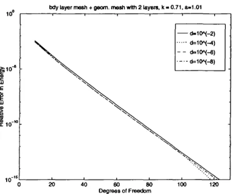
deal very successfully with this kind of singularity. A simple scaling argument suggests that the mesh should be chosen such that the ratio of the length of the elements to the dis-tance (of the elements) to the singularity is bounded from below. This can be achieved with geometric meshes of the type (24) where the number of layers L is such that the smallest element (xo, x\) has length proportional to dist(a, Q), i.e., aL ~ \a — 1|. For a = 015 and a = 101, we can choose L = 2 and for a — 1001 we may choose L = 3 to get aL ~ \a — \\. As the spaces S//(2, p) and S///(3, p) are based on the 'union' of these geometric meshes and the 'three-element' meshes, we expect these ansatz spaces to per-form well for the nearly singular cases a = 101 and a — 1001. We report the numerical results of the FEM with these ansatz spaces in Figs. 5, 6. We see that indeed this 'union' of the geometric mesh and the 'three-element' mesh leads to a very robust method both with respect to the perturbation parameter d and the parameter a.

6.2.2 The case a = 1. Let us now turn our attention to the limiting case a = 1. This case is of course no longer covered by the mathematical theory of this paper as the right-hand side is no longer differentiable at x = — 1. We study this case numerically because it is a simple one-dimensional model for various singularly perturbed elliptic-elliptic problems. For example, as alluded to in the introduction, the solution of the Reissner-Mindlin plate model with polygonal mid-plane has corner singularities. The limiting solution (as the thickness of the plate tends to zero) is the solution of the Kirchhoff plate equation. The solution of that equation also has corner singularities which are, however, of a different character than those of the Reissner-Mindlin equation.

10°

bdy layer mesh + geom. mesh with 2 layers, k « 0.71, a-1.01

510-iS £ HI

I

FIG. 5. Union of geometric mesh and three-element mesh; a = 101,2 layers

bdy layer mesh + geom. mesh with 3 layers, k = 0.71, a=1.001

I

• x

V

Degrees erf Freedom

120 140

598 J. M. MELENK

For a = 1, the solution u of (27) has a (weak) singularity at the left endpoint x = — 1: From (28) we see that the leading singular part of the solution u is

u (x + n2-045 (29)

(l-O45)(2-0-45)<^ U ( }

in an O(d) neighbourhood of x = — 1. On the other hand, as d tends to zero, the limiting solution is the singular function f\ which has a different, stronger singularity at x = — 1. It is reasonable to expect that the proper mesh should be such that it can resolve boundary layers, if present, that it can deal with the (weak) singularity at x = — 1 for d > 0, and that it can also resolve the stronger singular behaviour of the limiting solution f\. Functions of the type (29) and the limiting solution f\ are analytic on Q but have a singularity at the left endpoint. The approximation of such functions by the hp version of the FEM was analyzed by BabuSka & Gui (1986). The mesh proposed there is a geometric mesh where the number of layers is proportional to p, the polynomial degree. For our problem, we therefore advocate a union of the 'three-element' mesh and such a geometrically refined mesh.

Let us remark that the hp FEM analyzed by BabuSka & Gui (1986), which is based on geometric meshes with a number of layers proportional to p, has several noteworthy features. Firstly, exponential rates of convergence can be achieved in this way for the ap-proximation of singular functions of the type considered here. Secondly, the same geo-metric mesh achieves this exponential convergence for singular functions of the type (29) and f\ simultaneously. This is a very convenient feature of p or hp extensions. If singular functions are approximated using the h version of the FEM, the optimal, 'radical' meshes depend strongly on the type of singularity (cf BabuSka & Gui (1986)). Hence, an /i-version approach with optimal mesh design would be much more complicated in this situation as the type of mesh has to change as d tends to zero.

Let us return to the use of geometric meshes for our problem. Although the geometric meshes of BabuSka & Gui (1986) are optimal in some sense and lead to exponential rates of convergence, it is more convenient in practical applications to fix a mesh and increase the polynomial degree p. This approach is taken in the numerical experiments of Figs. 7, 8. In those computations, the perturbation parameter d is chosen as d = 10"4 or d — 10"6, and a 'union' of a geometric mesh at the left endpoint and a boundary layer mesh for the right endpoint is used, i.e., the finite element spaces are Sm(L, p) for various numbers of layers L. This 'union' thus takes care of the boundary layer at the right endpoint x = 1. As the mesh design at the left endpoint x = — 1 is independent of the perturbation parameter d, we cannot expect the finite element spaces S///(L, p) to perform completely robustly with respect to d. However, as soon as the number of layers L is O(\\x\d\), the smallest element of the geometric mesh is of size O(d) (cf Proposition 20, Remark 21); the dependence of the method on the perturbation parameter d is therefore rather weak as geometric meshes with few layers create elements of size O(d). For d = 10"4 or d = 10"6 and a = 015 already L =2, resp. L = 4, leads to meshes whose smallest element at the left endpoint is

O(d).

Because the mesh is fixed and the solution has a singularity at * = — 1, the asymptotic rate of convergence is algebraic and given by that of the p version of the FEM. For singular functions of the type (29), the analysis of BabuSka & Gui (1986) shows that the / / ' error of the smallest element behaves like p-W-o^s)-^ j e a rate of QQf-^2 for ^c asymptotic

10"

bdy layer mssh at right endpt fixed geom. mesh, a-1.0, efe1O"(-4)

10"' 10 2 layers — 4 layers Slayers Slayers \ \ \ \ \ \ 10" 10" 10' Degrees of Freedom 10*

F I G . 7. Geometric m e s h at x = — 1, boundary layer mesh at x = V,a = 1 0 , d = 10

10"

10"1

bdy layer mesh at right endpt, fixed geom. mesh, a-=1.0,

10 10 10' 2 layers 4 layers — 6 layers 8 layers 10 layers 10" 10" 10' Degrees of Freedom 10*

600 J. M. MELENK

error behaviour in the energy. Indeed, asymptotically, the error curves in Figs. 7, 8 are practically straight lines with slopes slightly over 4. However, depending on the number of layers, the pre-asymptotic range can be quite large: for example, in Fig. 7 with 6 layers, the asymptotic behaviour is not visible until the global error in energy is ~ 10~9. For a mesh with 8 layers, the asymptotic behaviour does not start until the energy error is 10~14. In this pre-asymptotic range the global error is not dominated by the error in the first element abutting on the singularity. Rather, the error reduction is determined by the error reduction possible in the elements away from the singularity. There, exponential rates of convergence (in p) are possible and this exponential rate of convergence is visible in the pre-asymptotic regime.

6.2.3 The final conjecture. We saw that in the case of an unsmooth right-hand side the use of a 'union' of a geometric mesh with a 'three-element' mesh is very successful. This is due to two facts. Firstly, 'three-element' meshes are designed such that the two small elements can resolve the boundary layers well. Secondly, geometric meshes can absorb both the singular behaviour of the solution for positive d as well as the singular behaviour of the limiting solution ford = 0. This 'union' of meshes is therefore very versatile.

For practical purposes, the introduction of small boundary layer elements is unnecessary at those boundary points towards which a strong geometric refinement is done because the geometric mesh leads to small elements of size O(d) with fairly few layers. For problems whose solution is not analytic up to the boundary (as in the case a = 1), the use of a fixed geometric mesh can, asymptotically, only lead to algebraic rates of convergence. However, the use of a sufficient number of layers ensures that the asymptotic behaviour of the p version is pushed beyond the practical ranges of polynomial degrees p, and we have the pre-asymptotic exponential convergence.

7. Concluding remarks

In the present paper, we analyzed the hp FEM for a one-dimensional singularly perturbed problem of elliptic-elliptic type. We showed that for analytic input data, the introduction of two small elements of size O(pd) near the boundary leads to robust exponential con-vergence of the hp FEM.

Although we considered a simple model problem, the techniques used here apply to more general situations. The essential tool for the proof of the approximation result The-orem 16 are classical asymptotic expansions for which the asymptotic part as well as the remainder can be controlled explicitly in terms of the perturbation parameter d and the expansion order M (Theorems 3, 6). Similar asymptotic expansions hold true for the convection-diffusion equation with analytic coefficients. The approximation result Theo-rem 16 holds therefore for the convection-diffusion equations with analytic coefficients as well. Of course, as the solutions of the convection-diffusion equation have a bound-ary layer at the outflow boundbound-ary only, it would be enough to use two elements where the small element is located at the outflow boundary. Let us conclude our remarks on the convection-diffusion equation by stressing that stability of finite element methods for the convection-diffusion equation is, as opposed to the reaction-diffusion equation considered in this paper, a non-trivial issue; a stable hp FEM for the convection-diffusion equation

able to make use of robust exponential approximability results of the type proved in this paper is presented by Melenk & Schwab (1997b).

Finally, the ideas developed in this paper are not restricted to one-dimensional problems; this is demonstrated by Melenk & Schwab (1997a) who successfully employ the ideas of the present paper for the construction of a robust, exponentially converging hp FEM for a reaction-diffusion equation in two dimensions.

We confirmed our theoretical result of robust exponential convergence by numerical ex-periments. Additionally, we studied numerically the case when the solution and the limit-ing solution (as the perturbation parameter tends to zero) are slimit-ingular. There, we advocated the use of a 'union' of the proper boundary layer mesh with a geometrically graded mesh which is able to absorb the singular behaviour of the solution and the limiting solution. We showed numerically that this approach leads to very satisfactory results.

Acknowledgement

Professor C. Schwab brought the problem considered in this paper to my attention, and I would like to thank him for his helpful discussions and suggestions.

REFERENCES

BABUSKA, I., & GUI, W. 1986 The p and hp versions of the finite element method in one dimension. Part I: the error analysis of the p version. Part II: the error analysis of the hp version. Numer. Math. 49,577-612 and 613-57.

ClARLET, P. G. 1978 The Finite Element Method for Elliptic Problems. Amsterdam: North-Holland. DAVIS, P. J. 1974 Interpolation and Approximation. New York: Dover.

MELENK, J. M.t & SCHWAB, C. 1997a hp FEM for reaction-diffusion equations. Part I: robust

exponential convergence. Part II: regularity. Research Reports 97-03 and 97-04, Seminar filr Angewandte Mathematik, ETH Zurich, CH-8092 Zurich, Switzerland.

MELENK, J. M., & SCHWAB, C. 1997b An hp finite element method for convection-diffusion prob-lems. Research Report 97-05, Seminar fur Angewandte Mathematik, ETH Zurich, CH-8092 Zurich, Switzerland.

MILLER, J. J. H., O'RIORDAN, E., & SHISHKIN, G. I. 1996 Fitted Numerical Methods for Singular

Perturbation Problems. Singapore: World Scientific.

MORTON, K. W. 1996 Numerical Solution of Convection-diffusion Problems. London: Chapman & Hall.

O'RIORDAN, E., & STYNES, M. 1986 A uniformly accurate finite-element method for a singularly perturbed one-dimensional reaction-diffusion problem. Math. Comput. 47,555-70.

ROOS, H.-G., STYNES, M., & TOBISKA, L. 1996 Numerical Methods for Singularly Perturbed Dif-ferential Equations. Berlin: Springer.

SCHWAB, C , & SURI, M. 1996 The p and hp version of the finite element method for a problem with boundary layers. Math. Comput. 65,1403-29.

SUNDERM ANN, B. 1980 Lebesgue constants in Lagrangian interpolation at the Fekete points. Ergeb-nisberichte der Lehrstiihle Mathematik 111 & Will (Angewandte Mathematik) 44, Universitat Dortmund.