Design and implementation of balance control in a humanoid robot

Design and Implementation of Balance Control in a Humanoid Robot by

Brendan J. Englot

SUBMITTED TO THE DEPARTMENT OF MECHANICAL ENGINEERING IN PARTIAL FULFILLMENT OF THE REQUIREMENTS FOR THE DEGREE OF

BACHELOR OF SCIENCE AT THE

MASSACHUSETTS INSTITUTE OF TECHNOLOGY JUNE 2007

©2007 Brendan J. Englot. All rights reserved.

The author hereby grants to MIT permission to reproduce and to distribute publicly paper arid electronic copies of this thesis document in whole or in part

in any medium now known or hereafter created.

Signature of Author:

SL of _{Department of Mechanical Engineering}

May 11, 2007

Certified by:

Accepted by:

Steve G. Massaquoi Ass iate rof sor of Electrical Engineering and Computer Science and Health Sciences & Technology Thesis Supervisor

N~)

il~

Professor of Mechanical Engineering Chairman, Undergraduate Thesis Committee

MASSACHUSETTS INSTIUTE.

OF TECHNOLOGY

JUN

2

12007

Design and Implementation of Balance Control in a Humanoid Robot By

Brendan J. Englot

Submitted to the Department of Mechanical Engineering on May 11, 2007 in partial fulfillment of the requirements for the Degree of Bachelor of Science in

Mechanical Engineering ABSTRACT

A proportional derivative control strategy was developed for the purpose of achieving balance in a humanoid robot. An artificial muscle model was adapted which modified physiological parameters for the purpose of controlling a lightweight robot skeleton. Gains were modified as a function of joint angles to permit low gain near the equilibrium point, and consequently to promote a human-like swaying behavior that is energy-efficient.

The control strategy was testing by placing a non-zero initial condition on the ankle joint angle and observing the robot, both physically and in simulation, attempt to achieve a stable swaying pattern. This was achieved successfully in a simulation of the robot's mass and inertial parameters, but further efforts must be made to obtain the same behavior in the robot.

The ability of a robot to successfully balance using a human-like sway pattern adds another successful biomimetic feature to humanoid robot control and in addition should improve the efficiency of such systems.

Thesis Supervisor: Steve G. Massaquoi

Title: Associate Professor of Electrical Engineering and Computer Science and Health Sciences & Technology

Table of Contents

1. Introduction...4

2.

Analysis

... ... 6

2.1 Balance Simulation...

...

2.1.1 Physical Plant...6

2.1.2 Control Strategy...10

2.2 Balancing the Robot...12

3. Materials and Methods...15

3.1 Apparatus...

...

15

3.2 Preparatory Work...17

3.3 Experimental Procedure...18

4.

Results...20

5. Discussion...23

Appendix A...

...

27

References

... .... 28

1.

Introduction

Bipedal locomotion is one of the richest and most challenging problems in the field of robotics today. There is currently no machine on two legs that can outrun or outmaneuver a human being, despite a robot's ability to transmit information many times faster than a human's nervous system. Were a bipedal robot capable of navigating rough and unpredictable terrain in a manner comparable or superior to that of a human being, a vast number of desirable applications would exist.

Perhaps for such a reason, a large body of research has focused on this topic, and consequently a wide variety of approaches have been taken in the design and control of walking robots.. One of the most celebrated achievements in this field is Honda's Asimo, which uses zero moment point (ZMP) control to keep the robot balanced by setting target ground contact positions and issuing corrective forces to attain those positions. An approach such as this is computationally intensive and functions poorly in an

unstructured environment. Asimo also consumes about ten times as much power as an equivalent walking human [Ramamoorthy and Kuipers, 2006].

On the other end of the spectrum, passive walkers have been developed which require no actuators, but nonetheless demonstrate a human-like gait pattern. Andy Ruina and his students at Cornell University have developed a 3-D passive dynamic walker with two legs and knees, possessing a combination of mass properties and geometric features which permit stable walking on a downhill slope [Collins, Wise, and Ruina, 2006]. Designs such as this provoke questions about the extent to which the human gait is the consequence of neural control or whether it is just the natural consequence of the mass and inertial properties of the human body.

Although a passive walker consumes far less power than an active walker, a robot such as Ruina's is still limited to very few environments in which it can operate stably. With the goal of de-emphasizing the need for precision, MIT's Leg Lab developed a series of robots in the 1980's and 1990's which employed series elastic actuators to aid in rejecting disturbances and reducing the need for precision actuators [Pratt et al, 1997]. By adding elasticity and reducing the need for precision, the Leg Lab's robots were biomimetic in some respects. As is often the case, emulation of nature's mechanisms can lead to a more efficient approach, and such efforts to mimic nature will lay the

groundwork for this study.

At MIT's Sensorimotor Neurocontrol group, a model of human neural control of movement has been developed which achieves robust walking in the sagittal plane in simulation [Jo and Massaquoi, 2006]. By modeling the suspected role of the cerebrum and cerebellum in the long-loop control of trunk pitch and center of mass position, a model that is largely otherwise feed-forward in nature is capable of generating a human-like gait. Aiding in the simplification of such a task, the feed-forward "neural input" generated by this model consists of only four unique spinal pulses which each

synergistically activate several muscles to produce a gait cycle comprised of five distinct phases (one of which is passive). The Sensorimotor Neurocontrol group currently aims to implement a similar control strategy in a robot, but there are several steps that serve as precursors to this task.

First and foremost, the robot must be capable of balancing freely while standing, doing so with a biomimetic model similar in basis to that which achieves walking in the sagittal plane. Such a model was developed in 2004 by the Sensorimotor Neurocontrol

group and proved robust against a variety of floor disturbances [Jo and Massaquoi, 2004]. It is anticipated that modifications to this model will be necessary for it to succeed in the

control of robot masses and inertias rather than human masses and inertias. This study aims to design a model which provides successful balance control of the robot while preserving as many biomimetic features as possible. First by achieving balance in simulation, and then in the actual robot, it is hoped that successful control of a behavior which relies entirely on feedback will serve as the cornerstone for developing more complex behaviors that can be executed using the same robot platform.

2. Analysis

2.1 Balance Simulation

The robot balance simulation is based on a control strategy developed with the intent of accurately modeling the role of the human cerebrum and cerebellum in maintaining balance [Jo and Massaquoi, 2004]. The model in this paper used FRIPID (force feedback recurrent integrator proportional integral derivative) control with gain scheduling to permit a human to recover balance from floor perturbations. The robot balance model takes a simplified approach, sacrificing biological accuracy in some respects to achieve robust balance control in a robot, rather than human, physical plant. The robot balance model dispenses with feedback transmission delays and the "recurrent integrator" stabilization path of the FRIPID model (transmission delays are likely to cause stability problems in a simpler model), and instead implements PD (proportional derivative) position control with gain scheduling and aims to achieve recovery from perturbations at the ankle.

The robot physical plant consists of feet, shins, thighs, a pelvis, and a spine and is designed to actively control ankle and knee pitch as well as pitch, roll, and yaw at the hip. The design of the leg is detailed in previous undergraduate thesis work [Chan, 2007]. A similar approach was used in the development of the hip. The robot physical plant is portrayed in Figure 1. Series elastic elements placed between hobby servos and the joints which they command serve as the robot's artificial muscle, providing some slack around the robot's rest position but capable of transmitting large forces when contracted.

The robot simulation captures an accurate estimate of plant inertial parameters using the Solidworks-to-SimMechanics Converter. In the world of SimMechanics, masses, energy storage elements, and mechanical constraints can be expressed in block diagram form to allow interfacing with control systems designed with Simulink. The

solid model pictured in Figure 2 was assigned mass properties and used as a physical plant capable of changing pitch atthe ankle, knee, and hip. Each joint was treated as having two opposing monoarticular muscles, modifying a muscle model developed for the simulation of human walking in the sagittal plane [Jo and Massaquoi, 2006].

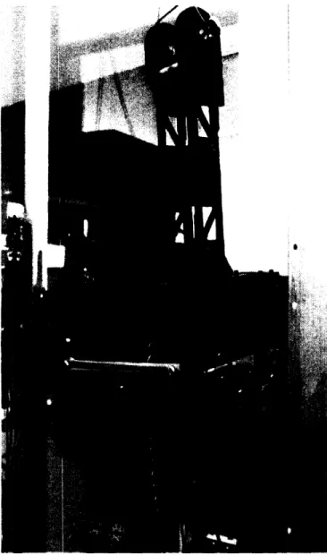
Fig. 1: A

photograph of the humanoid robot.

Fig. 2: The solid model of the robot

from which physical plant mass and inertia properties were estimated.

The muscle model assumes passive and active components of muscle force, such

that: F = Fpass+ Fact (1)

where the passive and active tension vectors are defined by equations (2) and (3).

Fpaov.. = Kpa,, (leq - 1) +Bpa,., 1 (2) F,1., = K ,,(lq - 1) +Bac, / (3)

If either force component sums to less than zero, then that force component is treated as zero in the simulation. The entries of the passive stiffness matrix (which exist along the diagonal only) were obtained by multiplying the estimated cross-sectional areas of the monoarticular "muscles" by a constant of 703.2 (as in the walking simulation paper). The active stiffness matrix was obtained by tripling each entry of the passive stiffness matrix, and each damping matrix was obtaining by dividing each entry of the respective stiffness matrix by ten. The values used as cross-sectional areas for muscles at the hip, knee, and ankle, were derived from estimated cross-sectional areas of the gluteus maximus (GM) , biceps femoris short (BFS), and soleus (SO), respectively. The cross-sectional areas of the GM and BFS were then reduced by a factor of ten, and the SO by a factor of one hundred to account for the reduced scale of the robot with respect to a human. These factors were determined empirically by observing the passive behavior of the robot skeleton and modifiying the muscle cross-sectional areas until human-like passive behavior was observed. The approximate lengths of the GM, BFS, and SO were also used in the model, and can be found in the appendix along with cross-sectional area values.

Changes in joint position and velocity were delivered to the muscle model after undergoing transformation from joint space to muscle space, representing these quantities as changes in muscle length and rate of change of muscle length. This transformation

took place using a 6x3 moment arm matrix (found in the appendix) which used estimated moment arms of the GM, BFS, and SO for transforming hip, knee, and ankle joint

commands respectively. This series of modifications to the muscle model [Jo and Massaquoi, 2007] resulted in a symmetric set of six monoarticular muscles scaled down in stiffness to suit a smaller and lighter body.

Once it is calculated using the muscle model, muscle force is transformed from muscle space back into joint space using the transpose of the above-mentioned moment arm matrix. This provides joint torque commands to the robot skeleton, which, as mentioned above, consists of mass and inertial properties obtained from the solid model in Figure 2. Torque is applied to each joint as if a motor were present at that joint, and the resulting changes in angular position and velocity at each joint are approximated using SimMechanics.

The SimMechanics model of the robot skeleton operates under the assumption that both feet are in complete contact with the ground at all times. In other words, it was assumed that the feet would not translate or rotate with the respect to the ground (and this constraint was imposed using SimMechanics). This is an assumption that is valid for small perturbations in the ankle joint angle from the vertical, but for larger angles does not hold true for a freely standing human. For angular displacements from the vertical on the order of five degrees, a human would require an external force to anchor his or her feet in order not to translate or rotate the feet from their initial position. Nonetheless, the appealing simplicity of such an assumption coupled with the fact that the displacements tested in this study are not large enough to cause such problems led to the adoption of this assumption for all simulated trials.

2.1.2 Control Strategy

As previously stated, the control strategy implements PD position control with gain scheduling to control joint angle position. A joint angle vector is fed back from the robot plant model and the error is operated on using proportional and derivative gains that are adjusted by a gain multiplication factor. The gain multiplier is a function of joint angle and is designed to promote the human-like feature of a back-and-forth sway during upright balancing rather than a dynamic model that freezes once it attains the desired position. In humans, this feature presumably saves energy by allowing muscles to relax

alternately during maintained upright posture. The gain multiplier function used in this paper was designed to allow gains to reach their maximum value at an error of plus or minus one degree, and it is displayed in both Figure 3 and equation (4).

G,,,,, = 0.5 * Itanh(2;r(6 + 0.5) + tanh(2xr(0 - 0.5)) (4) For attaining balance, the reference angles were set to 0 degrees at the ankle, knee, and hip joints. The proportional gain matrix used contained only two diagonal entries, a gain for the ankle and a gain for the knee. A gain for the hip was not required because the mass of the robot's trunk is quite small relative to that of a human's trunk, the passive stiffhess of the artificial muscle being enough to keep the robot's trunk stable. The entries of the derivative gain matrix were set to 75% of the values in the proportional gain matrix. Before operating on the position error vector, each gain was, as mentioned above, multiplied by the value of the function in equation (4). In the case of the

derivative gain, this multiplication occurred after the error signal was differentiated. After being operated on by each set of gains, the error signal, or "neural input", was converted from joint space (3x1) to muscle space (6xl) and each muscle stretch

I I

I

j2

/

2

Fig. 3: Gain multiplication factor as a function of joint angle (same for the ankle, knee, and hip joints).

command was filtered by a second-order low-pass filter detailed in equation (5). This step was included to model the activation of muscle force by neural input, which occurs according to low-pass dynamics [Fuglevand and Winter 1993].

p2

F(s)= p

(s + p)2 ( p =30 rad/s)

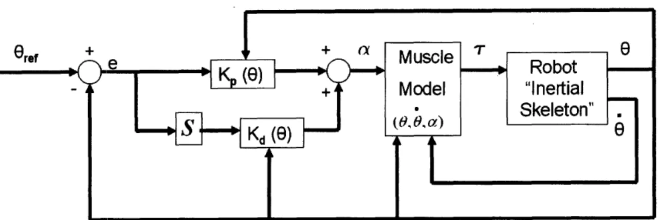
In addition to the "neural input" signal, a joint angle position vector and joint angular velocity vector (obtained from the "inertial skeleton") are fed into the muscle model. A diagram summarizing the control strategy is included in Figure 4.

t a c 0.8 -i

0.6

0.4

0.2

(5)

j

Fig. 4: A block diagram representing the control strategy used in the balance simulation, implementing PD

control with gains that change as a function of joint angle.

2.2 Balancing the Robot

Interacting with the robot physical plant requires servo position commands, despite the fact that the simulated physical plant is controlled with joint torques. In order to traverse from joint torque commands to servo position commands, a series of

operations is required, which is detailed in the block diagram of Figure 5. Joint torques must first be converted to linear "muscle" forces using the moment arm of the series elastic actuators at each joint. This requires a knowledge of the distance between the

Fig. 5: A block diagram which demonstrates the operations necessary to convert joint torque commands into robot servo position commands. Knowledge of the moment arm at each joint, the number of motors at each joint, the force required to eliminate slack in the series elastic actuator, the spring constant of the stiff spring, the radius of the servo horn, and the servo angular displacement required to eliminate slack are necessary in order to deliver accurate position commands.

point of force application of each artificial series elastic muscle and the center of rotation of the respective joint, as well as the angle that the artificial muscle wiring makes with this point of force application. After the total linear force along the muscles at each joint is estimated, it must be divided by the number of motors at each joint to obtain the linear force present in each individual series elastic muscle. The next series of steps involves accounting for the slack present in the series elastic actuator design.

As mentioned above, the series elastic elements possess a certain amount of slack at the target position (in the case of balance control, the target position is when the robot is standing up straight). This is due to the fact that the pair of elastic elements consists of one spring that is considerably compliant (191 N/m) and another that is considerably stiff (6355 N/m). The force-displacement curve of this series elastic element can be found in Figure 6. Before a set of servos at any given joint can force the joint to move, the servos must contract any artificial muscle to the point at which its slack is eliminated. In order to do this, the low stiffness spring must be completely compressed. Due to the fact that not all series elastic elements can be tensioned in precisely the same way, the servos commanding each joint require a slightly different amount of displacement before there is enough contraction to eliminate the slack zone. This requirement slightly complicates the servo position command needed to achieve a desired joint torque, requiring the two summations that are observed in Figure 5. First, the force required to contract the low stiffness spring is subtracted from the total muscle force command, to obtain the force required once the slack is eliminated. This remaining force is then divided by the high

N e c 40 -r o

F

a

Fig. 6: A force-displacement curve of the series elastic element used in the robot's artificial muscle.

stiffness spring constant to determine the contraction of the stiff spring that will be required to obtain the commanded force in the artificial muscle. This contraction

distance is then divided by the radius of the servo horn (the wheel attached to the face of the servo) to obtain the angular displacement of the servo corresponding to this

contraction. Finally, the angular displacement required to eliminate the series elastic slack is added back to this value to obtain the total displacement of the servo horn required to both eliminate slack and displace its respective joint by the amount

corresponding to the torque command. If this series of steps is carried out using accurate parameters, then the torque commands of the muscle model will be reflected in the

commanded displacements of the servo motor.

Joint positions of the robot will be recorded and fed back into the control strategy illustrated in Figure 4. The only difference between the simulated balance control and control of the actual robot will be that an actual robot will replace the robot "inertial

skeleton" used in the simulation. As a consequence, the torque commands generated by the muscle model must undergo the additional operations discussed in this section.

3. Materials and

Methods

3.1

Apparatus

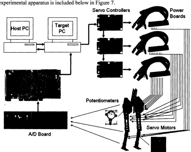
As the details of the physical plant design and fabrication have been discussed in previous work [Chan, 2007], this section will focus mainly on the apparatus used to control the physical plant. The analysis of balance control in the sagittal plane required the use of 20 servo motors, 2 at each ankle, 4 at each knee, and 4 at each hip, used in each case to control the pitch of the respective limb. The servos were controlled using 3 Pololu Serial 8-Servo Controllers (both the motors and the controllers were powered with 5V DC), and the controllers were commanded via serial communication with a "target PC" dedicated to the real time control of the physical plant. The target PC communicates via Ethernet with a host PC, which, using Simulink and xPC from Mathworks, compiles and sends control routines to the target PC. Servo power boards were used to deliver power to the servo motors independent of the servo controllers, although in these tests both were powered using the same supply.

Feedback was collected from the physical plant using potentiometers located at each joint on the right leg. The potentiometers were supplied with 9V DC and calibrated to read out the values of each joint angle in degrees. Joint angles were defined such that a value of zero corresponds to vertical orientation with respect to the lower adjoining limb. Rotations in the positive sense were defined as joint rotations bringing the limb of interest forward in pitch, and negative rotations the opposite. Joint angles were delivered to the target PC via the PD2-MF-64-400/14H A/D board from United Electronic

Industries. All signaling and sampling occurred at a rate of 1000 Hz. A diagram of the experimental apparatus is included below in Figure 7.

Servo Controllers Power Boards

t

A/D Board

Fig 7: A diagram depicting the apparatus used to control the robot, illustrating the flow of information from the target PC to the plant via servo motors, and back to the target PC via potentiometer signals.

Only changes in pitch were of interest, so the robot's ability to move in other directions was partially restricted. The motion of the hip yaw joint was limited by fastening a rubber band between hips on both the front and back of the robot. The spine itself was also suspended from above to prevent the robot from falling in the case of a failed attempt to balance. The spine was suspended with enough slack to allow testing in all desired configurations. In addition, hip roll was not restricted since unwanted rotation about the roll joints did not occur. A photograph of the 3 degree-of-freedom hip

The apparatus used in running the balance simulation consisted of only a single PC, which ran the simulation using MATLAB. Simulink, and SimMechanics from Mathworks. The control strategy implemented in simulation differed only in the respect that its torque commands were delivered to a simulated physical plant rather than the actual robot physical plant.

3.2 Preparatory Work

In order to prepare the apparatus for testing, a number of steps took place over the course of the last five months. A PC was sequestered for the purpose of being our target PC and Mathworks xPC was configured on this computer. Several weeks were spent

Fig. 8: The robot hip as it appeared during testing, hung firom the spine (with some slack) with the hip yaw joints partially immobilized.

trying to use xPC and Simulink to successfully communicate with our servo controller, and many simple Simulinnk models were created for the purpose of testing and

calibrating servo motors and potentiometers. Much effort was also dedicated to

daisychaining the servo controller boards to distribute the serial input signal to multiple servo controllers. Much time was also dedicated to preparing the robot physical plant, including the robot assembly, tuning of series elastic actuators, and machining of parts.

3.3 Experimental Procedure

The ability of the robot to balance with a non-zero initial condition on the ankle joint angle was tested both in simulation and on the actual robot. A single set of gains was desired that would permit the robot to achieve stable balance with sway under a variety of initial conditions, and under both positive (forward) and negative (backward) initial displacement for each condition. It was anticipated that a different set of gains would be needed for the actual robot and for the simulated robot, since the biological estimates of muscle impedance used in the simulation differ from that of the series elastic actuators in the robot.

The precise initial conditions tested were ankle angles of positive and negative 0.02 radians (1.15 degrees) as well as positive and negative 0.01 radians (.57 degrees). The initial conditions at the knee and hip were always set to zero degrees. While running the simulation, a VR visualization of the balancing robot created using the MATLAB VR toolbox was used as a quick check to see whether the gains being tested attained stable balance with sway. A view of the VR visualization is available in Figure 9. In addition, ankle torque was monitored with a Simulink scope. Proportional and derivative gains were repeatedly adjusted using these visual features of Simulink. Not only was the visual

appearance in the VR visualization considered, but the numerical values of ankle torque as well, to ensure that the simulation was commanding realistic torque values.

Though the initial conditions on the actual robot could not be set as precisely as in the case of the simulation, they were set as accurately as possible by hand, and both the servo boards and servo motors were turned on before the control routine was initiated. The control routine was turned on while the robot was held with one hand in its initial position, and the hand was removed as soon as it was clear that the simulation was running. The common form of output available from both the simulation and the

Fig. 9: A 3-D virtual reality visualization used to quickly assess the affects of parameter changes on balance control.

physical testing are joint trajectory histories of the robot's attempts to balance, and these measures of performance will be analyzed shortly.

4. Results

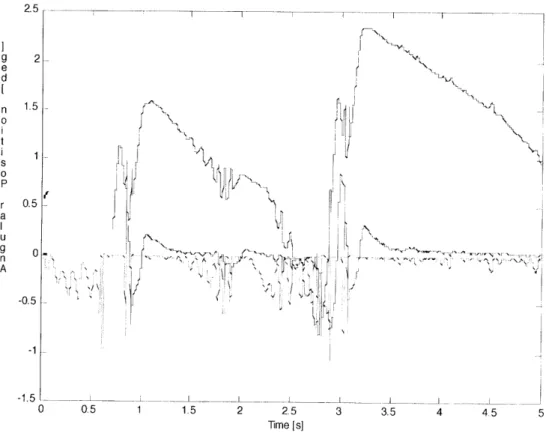
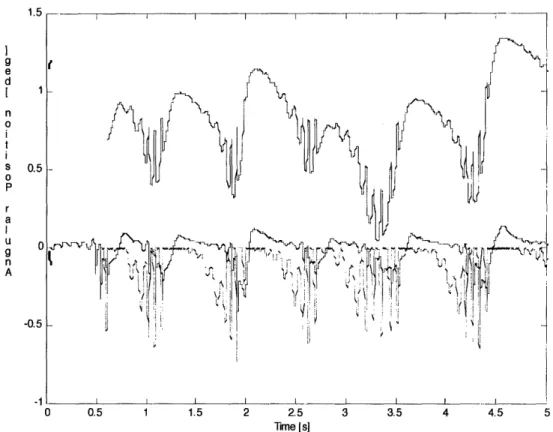
Figures 10-13 depict the time history of joint angles of the simulated robot in response to a variety of initial conditions. The response in Figure 10 represents an initial ankle angle of .01 radians, Figure 11 an initial ankle angle of -.01 radians, and Figures 12 and 13 represent initial ankle angles of .02 and -.02 radians, respectively. The feature of greatest interest in these graphs is the response of ankle angle, which varies significantly with changing initial conditions. In the case of Figure 11, a small, negative initial position resulted in a very uniform response that is sinusoidal in appearance. On the other hand, a small, positive initial position resulted in a response that appears to have a growing ankle angle peak. Doubling this initial position once again produces a uniform response, as illustrated in figure 12. And the response to a larger, negative initial condition is less uniform in appearance than that for a smaller initial condition.

Unfortunately joint trajectories could not be obtained from the actual robot for comparison. Upon implementation of this control strategy, a few unexpected behaviors were observed in the robot. Despite applying the same control strategy and

approximately the same initial conditions to the robot, some kicking behaviors resulted that brought the robot's feet off of the ground. Even when the proportional and

derivative gains were reduced by a factor of 100, this behavior continued to result. Since the robot would not balance, its joint trajectories are not visualized here. These

observations, although not the result that was hoped for, provide some valuable insight into why the balance control strategy did not succeed when applied to the robot.

riK

1.5 2

1.5 2 2.5

Time [s]

3 3.5 4 4.5 5

Fig. 110: _{Ankle (blue), knee (red), and hip (green) trajectories corresponding to}

an iniitial ankle position of.01 radians (0.57 degrees).

--- --- i---'Nd

*j

Fig. 11: Ankle (blue), knee (red), and _{hip (green) trajectories corresponding to}

an initial ankle position of-.01 radians (-0.57 degrees).

-0.5 0 0.5 4.5 5 ~, ~I I

i-si

yVI\A ~IIIIIU. ~I\~~~LTli.

II ri I ' ~~· ,·· i i L*l i:!

f

lij

R:

11i

g 9 e d [ 1 n 0 t s 0.5 P r a U ₀

9

Fig. 12: Ankle (blue), knee (red), and hip (green) trajectories corresponding to an initial ankle position of.02 radians (1.15 degrees).

e n 0 t 1.5-S ,-P 1--a I 0.5-U g 0x -0.5 V -1n -+ -1.5l ,' - \- I /\ ,\__ 0 0.5 1 1.5 2 2.5 3 3.5 4 4.5 5 Time [s]

Fig. 12: Ankle (blue), knee (red), and hip (green) trajectories corresponding to an initial ankle position of-.02 radians (-1.15 degrees).

1 r5

I.

5. Discussion

Despite the fact that the control routines run on the actual robot did not yield meaningful quantitative results, it nonetheless provides insight into reasons why the controller could not control the actual robot. In addition, the incongruence among the simulated ankle trajectory results reveals information about the asymmetries present within the robot skeleton, as well as the successes and failures of this control system.

One of the most surprising results obtained by the simulation is the unstable appearance of the ankle trajectory resulting from an initial position of .01 radians (Figure 10). This is a surprising result because an initial position of .02 radians, a deviation from the reference angle that is twice as large as that in Figure 10, yields an ankle trajectory that is far more uniform and stable in appearance (Figure 12). This provides evidence in favor of the stability of the response of Figure 10, which is a response whose infinite behavior is perhaps more complex than the portion of the response displayed in Figure 10. Throughout the process of testing controller gains, responses were encountered that exhibited unique and unexpected changes in behavior long after the simulation had begun. Several instances were observed in which a large, unstable-looking surge of motion actually served to stabilize the robot skeleton temporarily. Behavior such as this may be induced by the nonlinearity in the muscle model. Even though time delays have been removed from this model, instability is still possible if the neural input is high in frequency (due to the phase lag of the low-pass filter), so we cannot rule out instability as a possibility.

The ideal, anticipated ankle trajectory is best summarized by Figure 11, a response that began at an initial position of -.01 radians. The ankle trajectory curve in

this figure consists of uniform, repeating bumps. The robot simulation appears to have found a steady state in which it sways uniformly from a position of about .25 degrees to 1 degree and back. This is a behavior that was anticipated due to the existence of the gain multiplier function, which, at positions near zero, cuts down the values of the gains and

leaves more slack in the robot's "muscles".

Another good example of the anticipated trajectory can be found in Figure 12, whose response had an initial position of .02 radians. This response also displays

trajectory bumps which are close to uniform in amplitude and duration, as the robot again sways back and forth from a position of about .25 degrees to a position of 1 degree. It is encouraging that this uniform ankle trajectory response was observed after both a positive and negative displacement from the vertical, since it demonstrates that a single set of gains can correct two inherently different disturbances (different because the skeleton is not symmetric about the vertical), and that a balance controller has the potential to be robust in controlling this physical plant.

Yet another fascinating piece of information contained within the trajectory curves is that for each initial displacement, there appears to be a unique equilibrium point about which the robot sways. Although no curve has the exact same equilibrium point, every response, whether the initial position was positive or negative, sways about a positive equilibrium point. This is likely to be a consequence of our choice of controller, which uses only proportional and derivative control. Although the gain multiplier results in sway for infinite time, this equilibrium point is the point to which the position would settle to if the gains were constant. If integral control were to be added to the robot's control strategy, then it is likely that this equilibrium point would be shifted to zero, due

to the effective elimination of steady state error.

Although Figures 10 and 13, with trajectories whose "sway bumps" are less uniform in magnitude and duration, might detract from the claim that this is a robust controller, they also provide us with information about the inner workings of the control strategy. These figures contain a shape of bump that is different from that observed in Figures 11 and 12, as it is taller, wider, and it is clearly asymmetrical. It is likely that a position change of such high magnitude is occurring as a result of the nonlinearity in the muscle model. It is speculated that this nonlinearity is also responsible for the high frequency content that is observable throughout the position response curves. Small amounts of chatter (perhaps due to the location of equilibrium points for different limbs at different angles) appear to be getting amplified by this nonlinearity, finding their way into the position response. This model would benefit from a closer investigation of the effects of the nonlinear muscle model in future work.

With regard to the attempted control of the actual robot, a few educated guesses can be made from the difficulties encountered in trying to control the physical plant. When this strategy was implemented, the legs tended to lift off the ground and kick rather violently. This is an indication that perhaps the assumption that the feet remain securely planted on the floor is not a good one after considering the magnitude of the torques

experienced at the ankle. If the simulation is using unnaturally high torques to keep the robot skeleton balanced, then this might be the source of failure. One reason why ground contact may have been especially poor in the trials conducted here is the fact that the spine was tied off and suspended from above. This relieved a good portion of the robot's weight and is likely to have significantly cut down the amount of tangential force

required for the robot's feet to begin slipping. In addition to this, there are numerous other potential sources of error, especially in the operations performed on joint torque commands to obtain servo position commands. If estimations about the distance required to eliminate series elastic slack were incorrect, then that may have caused certain servos to move too far in response to torque commands. The first step necessary will be to improve the robot's ground contact while still keeping the chances of a falling low, and then to debug the series of operations which transforms joint torques into servo position commands.

Despite failure to reproduce the results of the balance simulation in the actual robot, this investigation has succeeded in a few important ways. First, a method of balance control has been established which permits a natural sway about the equilibrium point, rather than causing the robot to come to a rigid stop. This feature makes this model more biomimetic, and, as is usually implied by this, more energy-efficient in nature. Second, for at least two of the investigated initial ankle positions, a position response very uniform in appearance was obtained, which, once the initial disturbance is corrected, appears to exhibit a steady-state pattern of sway. Future investigation will not only be centered on attaining balance in the actual robot, but also on improving the simulation to attain a truly robust controller which produces a steady state sway in response to a greater variety of disturbances.

Appendix A

Kp = [185 0 0; 0 185 0; 0 0 0] Kd = .75*Kp

Moment Arm Matrix = [0 0 .132; 0 0 -.132; 0 -.049 0; 0 -.049 0; .036 0 0; -.036 0 0] Passive Stiffness Matrix = diag(2.1378, 2.1378, 2.1097. 2.1097, .4079, .4079) Effective Muscle Lengths: GM = .35m, BFS = .26m, SO = .3m

References

Chan, Nathaniel K. (2007) Design and Implementation of Series Elastic Actuation in a Biomorphic Robot Leg. SB Thesis, MIT

Collins, S.H., Wisse, M., Ruina, A. (2001) A 3-D Passive Dynamic Walking Robot with Two Legs and ]Knees, International Journal of Robolics Research, 20 (7):607-615. Fuglevand AJ, Winter DA (1993) Models of recruitment and rate coding organization in motor-unit pools. J Neurophysiol 70(6):2470-2488

Jo, S., Massaquoi, S., (2006) A model of cerebro-cerebello-spinomuscular interaction in the sagittal control of human walking. Biological Cybernetics.

Jo, S., Massaquoi, S., (2004) A model of cerebellum-stabilized and scheduled hybrid long-loop control of upright balance. Biolgical Cybernetics, 91, 188-202.

Ramamoorthy, S. and B. Kuipers. (2006). Qualitative hybrid control of dynamic bipedal walking. In Proceedings of the Engineering Student Research Conference (GAIN 2006), University of Texas at Austin.