Computational imaging and analysis in breast cancer

Computational Imaging and

Cancer

MASO TE

by

_MAR

₀₆

₂₀₁₈

Justin Lee

_LIBRARIES

Submitted to the Department of Health Sciences and Technology

ARCHIVES

in partial fulfillment of the requirements for the degree of

Doctor of Philosophy in Health Sciences and Technology

at the

MASSACHUSETTS INSTITUTE OF TECHNOLOGY

February 2018

@

Massachusetts Institute of Technology 2018. All rights reserved.

Signature redacted

A uthor ...

Department of Health/ ciences and Technology

Feb 1, 2018

Signature redacted

C ertified by ...

George Barbastathis

Professor of Mechanical Engineering, MIT

Thesis Supervisor

Signature redacted

A ccepted by ...

...

Emery N. Brown

rofessor of Health Sciences and Technology and

Professor of Computational Neuroscience, MIT

Director, Harvard-MIT Program in Health Sciences and Technology

77 Massachusetts Avenue Cambridge, MA 02139

MfTLibraries

http://Iibraries.mit.edu/ask

DISCLAIMER NOTICE

Due to the condition of the original material, there are unavoidable flaws in this reproduction. We have made every effort possible to provide you with the best copy available.

Thank you.

The images contained in this document are of the best quality available.

Computational Imaging and Analysis in Breast Cancer

by

Justin Lee

Submitted to the Department of Health Sciences and Technology on Feb 1, 2018, in partial fulfillment of the

requirements for the degree of

Doctor of Philosophy in Health Sciences and Technology

Abstract

The conventional pathologic analysis of malignancies involves a qualitative charac-terization and integration of several factors including tumor size, general degree of differentiation, tumor heterogeneity, mitotic rate, and lymphovascular invasion. For some cancers, biomarkers such as hormone receptor expression or receptor kinase over-expression can provide additional prognostic and therapeutic guidance. Unfor-tunately, all of these qualitative histologic approaches, while generally accepted for directing patient care, often exhibit significant inter-observer variability resulting in inconsistent inter- and intra-institutional predictions of tumor behavior (including metastases and/or recurrence), resulting in incorrect diagnoses or treatment.

Because cellular morphology is an integrated reflection of genetic and epigenetic expression, we hypothesize that a more accurate quantitative accounting and mea-surement of histologic features can provide a more robust and reliable prediction of tumor behavior. Computational imaging utilizes software to augment or replace the role of traditional optical elements in imaging systems and has an ability to signif-icantly increase the accuracy, robustness and cost-efficiency of digital pathology. In this thesis, we develop and test three novel computational imaging algorithms in-cluding, to the best of our knowledge, the first system for lensless computational imaging through deep learning. We then test our hypothesis by applying augmented image retrieval, analysis algorithms, and machine learning on a validated dataset of breast cancer images where the clinical outcomes of the primary tumor are known. In particular, we analyze algorithms related to identifying mitoses as a central proof of concept.

Thesis Supervisor: George Barbastathis

Title: Professor of Mechanical Engineering, MIT

Acknowledgments

I dedicate this work to my loving wife, Diana, and my son, Liam.

This work would not have been possible without the help and support of a mul-titude of people.

First and foremost, I would like to thank my research advisor, Professor George Barbastathis for high incredible kindness, mentorship, and patience with me while I meandered through graduate studies.

I would like to thank my committee members, Professor Richard Mitchell and

Professor Timothy Padera for taking an interest in my research and for serving on my committee. I have greatly appreciated your clinical insights and advice.

I would like to thank Irina Gaziyeva for the amazing work she has done behind the scenes to allow our group to focus more on research and less on paperwork.

I am grateful for all of my past and present labmates in the 3D optical systems group: Yuan Luo for teaching me the basics of experimental laboratory optics. Laura Waller for introducing me to OSA "optics fun day" and mentoring me early on. Yi Liu, Nader Shaar, Nick Loomis, Jose A. Dominguez-Caballero, Se Baek Oh, Hyungryul Choi, Hanhong Gao, Jonathan Petruccelli, Max Hsieh, and Jeong-gil Kim for helpful office discussions (sometimes on labwork and many other times on totally unrelated matters).

I would like to thank Zhengyun Zhang for his helpful comments and insights at group meeting and Ayan Sinha for patiently explaining questions I had on deep learning.

I would like to give an extra special thanks to Lei Tian and Shuai Li for their help with research.

I am grateful to my former HST classmates: Adam Pan, Kelli Xu, Nikhil Vad-havkar, Vyas Ramanan, and Andrew Warren for being amazing friends, even when I am horrible at keeping in contact with people.

Outside of lab, I would like to thank Bill Herrington for optics teaching demo discussions.

I am grateful for the Computational Science Graduate Fellowship which has spon-sored my intellectual curiosity over the course of my studies.

Finally, I would like to thank the community at MIT. I have been a student at MIT for over a third of my life and consider it my second home. Although I'm eager to begin the next chapter of my life, I will always look back upon my tenure at MIT with the fondest of memories.

Contents

1 Introduction 23

2 Clinical Motivations 25

2.1 Breast cancer and its clinical management . . . . 25

2.1.1 R isk Factors . . . . 25

2.1.2 Screening . . . . 26

2.1.3 Classification and Treatment . . . . 26

2.2 Whole-slide imaging . . . . 28

3 Background Theory 31 3.1 Classical Microscopy . . . . 31

3.1.1 Brightfield and Phase Contrast Microscopy . . . . 31

3.1.2 _{Numerical Aperture, Magnification, Space Bandwidth Product,} D epth of Field . . . . 32

3.2 Computational Imaging . . . . 33

3.3 Regularization and Sparsity Priors . . . . 34

3.3.1 Compressive Sensing . . . . 34

3.3.2 Low-rank matrix recovery . . . . 36

3.4 Deep Learning . . . . 37

4 Regularized Phase Space Imaging Using Sparsity Priors 41 4.1 Phase-space in optics . . . . 41

4.2 Phase-space tomography . . . . 43

4.2.1 Introduction . . . . 4.2.2 Theory and Method . . . .

4.3 Denoised Wigner distribution deconvolution via low-rank matrix com-p letio n . . . . 4.3.1 4.3.2 4.3.3 4.3.4 4.3.5 4.3.6 Introduction . . . . Wigner distribution deconvolution . Noise considerations in WDD . . . Noisy matrix completion . . . . Comparison of techniques for WDD Discussion/ Conclusion . . . . . . . . 48 49 . . . . 55 57 . . . . 60 . . . . 62 5 Lensless Computational Imaging via Deep Leaning

5.1 Computational Imaging Techniques . . . .

5.1.1 In-line Digital Holography . . . . 5.1.2 Iterative Phase Retrieval: Gerchberg-Saxton Fienup Algoril

5.1.3 Transport of Intensity Imaging . . . .

5.1.4 Deep Learning Transport of Intensity Imaging . . . .

5.2 Lensless computational imaging through deep learning . . . . 5.2.1 Introduction . . . .

5.2.2 Experim ent . . . .

5.2.3 Results and Network analysis . . . . 5.2.4 Conclusions and discussion . . . .

5.3 Future W ork . . . . 6 Computational Imaging for Mitosis Detection

6.1 Ptychography and Fourier Ptychography . . . .

6.1.1 Ptychography . . . .

6.1.2 Fourier Ptychography . . . .

6.1.3 Experimental Fourier Ptychography . . . . 6.1.4 Fourier ptychographic imaging through turbid media . . . 6.2 MIToscope: Automated mitosis detection in a desktop microscope

thm 65 65 66 66 68 68 70 70 75 79 81 82 91 92 92 94 95 96 97 44 45 48

6.3 Deep learning mitosis detection from focal stack images . . . . 6.3.1 Dataset/Methods . . . . 6.3.2 T raining . . . . 6.3.3 R esults . . . . 7 Concluding Thoughts A Supplemental Material A.1 Calibration . . . . A.2 DNN Training . . . . A.3 Axial perturbation, lateral perturbation and rotation at

training distances . . . . A.4 Linear phase modulation . . . .

other two 9 99 99 101 102 109 111 111 113 115 118

List of Figures

3-1 4f system . . . . 31 3-2 Compressive Sensing Reconstruction based on knowledge that an

un-derlying signal is "sparse". (left) L2 minimization "grows a circle" until

it touches the plane of possible solutions, yielding an incorrect answer. (middle) Lo minimization "searches along the axes" and would yield the correct solution but is NP-hard. (right) L1 minimization "grows

a diamond" and reaches the same solution as the LO norm with over-whelming probability in cases where the measurements are incoherent with each other and the restricted isometry property is satisfied. . 35

3-3 Each neuron in an ANN multiplies its inputs by a pre-established

weights, then sums the weighted inputs together and passes the sum through a nonlinear activation function. Common activation function include the sigmoid function and rectified linear unit. . . . . 38

3-4 Artificial Neural Network . . . . 38 3-5 CNN for classification. At the very last layer of the CNN, the values

represent an input's classification state likelihood. . . . . 39 3-6 LeNet, ResNet, and DenseNet are common DNN architectures. ... 40 4-1 A temporal spectrogram (musical score) provides more insight into

audio signal than a Fourier Transform of the entire signal can . . . . 42

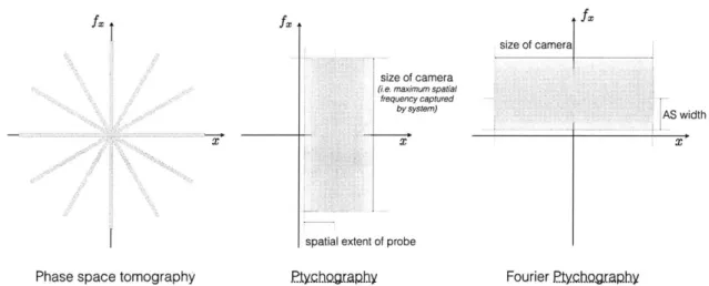
4-2 Phase-space tomography, ptychography, and Fourier ptychography in Phase-space . . . . 42

4-3 Experimental setup for WDD. A shifted probe is imaged onto the ob-ject plane and the resultant field p(x - si) - o(x) is propagated to a

Fourier plane where its intensity is measured. . . . . 50

4-4 Effects of a probe with limited spatial extent and limited bandwidth on object reconstruction in WDD. (Left) Actual Wigner distribution of object. (Top Center) Wigner distribution of a finite-extent probe. (Top Right) Wigner distribution of a band-limited probe. (Bottom Center) Recovered Wigner distribution of object using finite-extent probe. (Bottom Right) Recovered Wigner distribution of object using band-lim ited probe. . . . . 53

4-5 Effects of a probe with limited spatial extent and limited bandwidth on mutual intensity reconstruction in WDD. (1) Wigner distribution of object: (a)actual (b)retrieved using probe with limited spatial extent, (c)retrieved using probe with limited bandwidth. (2) sheared mutual intensity of object, o*(xi)o(xi + x): (a)actual (b)retrieved if probe has limited spatial extent, (c)retrieved if probe has limited bandwidth, (3) sheared mutual intensity of object's Fourier Transform, O(u)O*(u-s'):

(a)actual (b)retrieved if probe has limited spatial extent, (c)retrieved if probe has limited bandwidth . . . .54

4-6 Flow chart of denoised WDD with LRMC using modified SVT. Appli-cation of our algorithm to a simulated noisy l-D dataset with a band-limited probe yields a denoised rank-1 mutual intensity reconstruction similar to rightmost image (matrix is simultaneously completed and denoised). . . . . 60

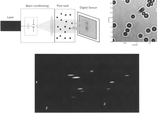
4-8 Results of WDD using: LRMR/LRMC, projection method from [67], and PIE at different noise levels. From left-to-right, the columns repre-sent: moduli (1-3) of reconstructed object using LRMR/LRMC, "pro-jection method", ptychography, and phase (4-6) of reconstructed object using LRMR/LRMC, "projection method", ptychography. The rows represent the total photon counts available to the detector in a shot-noise limited imaging system. . . . . 62 5-1 "Compressive holographic inversion of particle scattering." (top left)

In-line DH experimental setup. A 3D scattering potential of bubbles in water was reconstructed (bottom) from a single 2D snapshot (top right) using compressive holography. . . . . 67 5-2 Deep Learning Transport of Intensity Imaging . . . . 69 5-3 Deep Learning Transport of Intensity Imaging . . . . 70

5-4 Experimental arrangement. SF: spatial filter; CL: collimating lens; M: mirror; POL: linear polarizer; BS: beam splitter; SLM: spatial light m odulator. . . . . 76 5-5 DNN training. Rows (a) and (b) denote the networks trained on

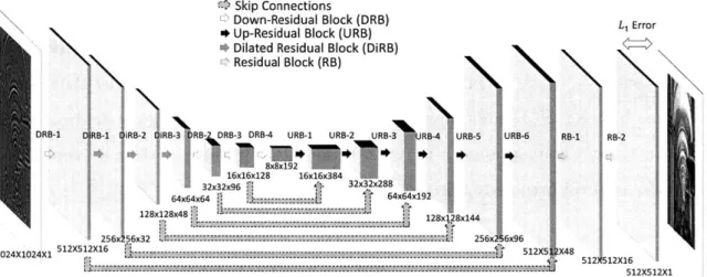
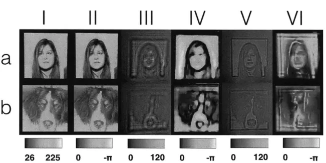
Faces-LFW and ImageNet dataset, respectively. (i) randomly selected exam-ple drawn from the database; (ii) calibrated phase image of the drawn sample; (iii) diffraction pattern generated on the CMOS by the same sample; (iv) DNN output before training (i.e. with randomly initial-ized weights); (v) DNN output after training. . . . . 77 5-6 Detailed schematic of our DNN architecture, indicating the number of

layers, nodes in each layer, etc. . . . . 78 5-7 Quantitative analysis of our trained deep neural networks for three

object-to-sensor distances (a) zi, (b) z2, and (c) z3 for the DNNs trained

on Faces-LFW (blue) and ImageNet (red) on seven datasets. (d) The training and testing error curves for network trained on ImageNet at distance z3 over 20 epochs. . . . . 83

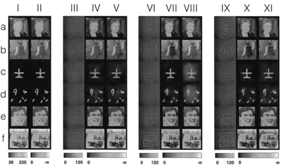
5-8 Qualitative analysis of our trained deep neural networks for combina-tions of object-to-sensor distances z and training datasets. (i) Ground truth pixel value inputs to the SLM. (ii) Corresponding phase images calibrated by SLM response curve. (iii) Raw intensity images cap-tured by CMOS detector at distance z1. (iv) DNN reconstruction from

raw images when trained using Faces-LFW [102] dataset. (v) DNN reconstruction when trained used ImageNet [120] dataset. Columns (vi-viii) and (ix-xi) follow the same sequence as (iii-v) but in these sets

the CMOS is placed at a distance of z2 and z3, respectively. Rows

(a-f) correspond to the dataset from which the test image is drawn: (a) Faces-LFW, (b) ImageNet, (c) Characters, (d) MNIST Digits, (e) Faces-ATT [86], or (f) CIFAR [108], respectively. . . . . 84

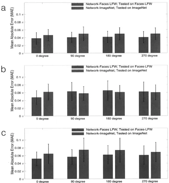
5-9 Quantitative analysis of the sensitivity of the trained deep convolu-tional neural network to the object-to-sensor distance. The network was trained on (a) Faces-LFW database and (b) ImageNet and tested on disjoint Faces-LFW and ImageNet sets, respectively. The nominal

depths of field for the three corresponding training distances zi, z₂, z3,

respectively, are: (DOF)₁ = 1.18 0.1mm, (DOF)2 = 3.82 0.2mm,

and (DOF)3 = 7.97 i 0.3mm. . . . . 85

5-10 Quantitative analysis of the sensitivity of the trained deep

convolu-tional neural network to laterally shifted images on the SLM. The network was trained on (a) Faces-LFW database, (b) ImageNet and tested on disjoint Faces-LFW and ImageNet sets, respectively. .... 86 5-11 Quantitative analysis of the sensitivity of the trained deep

convolu-tional neural network to rotation of images on the SLM. The baseline distance on which the network was trained is (a) zi, (b) z2 and (c) z3,

respectively. . . . . 87 5-12 Qualitative analysis of the sensitivity of the trained deep convolutional

neural network to the object-to-sensor distance. The baseline distance on which the network was trained is zi. . . . . 88

5-13 Qualitative analysis of the sensitivity of the trained deep convolutional

neural network to lateral shifts of images on the SLM. The baseline distance on which the network was trained is zi. . . . . 88

5-14 Qualitative analysis of the sensitivity of the trained deep convolutional neural network to rotation of images in steps of 90. The baseline dis-tance on which the network was trained is z,. . . . . 89

5-15 Failure cases on networks trained on Faces-LFW (row a) and ImageNet

(row b) datasets. (i) Ground truth input, (ii) calibrated phase input to

SLM, (iii) raw image on camera (iv) reconstruction by DNN trained on

images at distance z, between SLM and camera and tested on images at distance 107.5 cm, (v) raw image on camera and (vi) reconstruction

by network trained on images at distance z3 between SLM and camera

and tested on images at distance 27.5 cm. . . . . 89

5-16 (1) 16 x 16 inputs that maximally activate the last set of 16

convo-lutional filters in layer 1 of our phase retrieval network trained on ImageNet at distance of zi, a deblurring network, and an ImageNet classification network. The deblurring network was trained on images undergoing motion blur in a random angle within the range [0,180] de-grees and a random blur length in the range [10,100] pixels. The image is downsampled by a factor of 2 in this layer. (2) 32 x 32 inputs that maximally activate the last set of 16 randomly chosen convolutional filters in layer 3 of: our network, the same deblurring network, and the ImageNet classification network. The raw image is downsampled by a factor of 8 in this layer. . . . . 90

6-1 In ptychography, an illuminating probe function is scanned over a sam-ple and propagated to an output plane. . . . . 92

6-2 Phase retrieval using the extended Ptychographic Iterative Engine. By enforcing consistency in overlapping regions' measurements, both the probe function and object function can be simultaneously retrieved using the ePIE. (left) object estimate at early stage of ePIE algorithm, (middle) object estimate at later stage of ePIE algorithm (right) final object estimate from ePIE algorithm. . . . . 93 6-3 Fourier Ptychography Imaging Setup. . . . . 94 6-4 In Fourier Ptychographic Microscopy, many low resolution images

(cap-tured using different angles of illumination) are synthesized into a single higher resolution im age . . . . 95 6-5 Fourier Ptychographic Image Reconstruction. (left) object estimate at

early stage of algorithm progression, (middle) object estimate at later stage of algorithm, (right) "ground truth" image . . . . 96 6-6 Fourier Ptychographic Image Reconstruction of onion root tip. (left)

raw low-resolution on-axis image fed into ePIE algorithm, (right) high-resolution ePIE reconstruction . . . . 97 6-7 Fourier ptychographic imaging through turbid media. . . . . 98 6-8 Fourier ptychographic imaging through turbid media. Top-to-bottom

image pair progression shows the algorithm's current estimates for P1 (left) and P2 (right) over time . . . . 103 6-9 Example MIToscope setup. In the setup on the right, an LED

ar-ray was inserted into the standard brightfield setup to allow Fourier ptychographic imaging. . . . . 103 6-10 Onion cells in various states of cell cycle. . . . . 104

6-11 Automated onion cell mitosis detection. (top) full field of view/single

image (bottom) zoomed-in field of view . . . . 104

6-12 2.5p over-focused, 2.5p underfocused, and in-focus images were used

to train our DNN . . . . 105 6-13 Noise added to images to simulate equal photon budget. . . . . 105

6-14 First training set drawn from labeled image. (top-right) cropped im-ages centered at mitoses pixels (bottom-right) randomly selected non-m itoses pixels . . . . 105 6-15 The probability map generated by a DNN trained using set A has a

high false-positive rate. (left) ground truth image with mitoses labeled in yellow. (right) mitosis probability map (darker = higher probability) 106

6-16 Training set B was generated using cropped images centered at mitoses

pixels (top right) and non-mitoses (bottom right) pixels selected from a weighted probability distribution proportional to the probability map generated by the DNN trained using training set A (left) . . . . 106 6-17 (left) ground truth image with mitoses labeled in yellow. (right)

Ex-ample DNN output when trained using training set B. Green circles denote correctly identified mitoses; the red circle indicates a missed m itoses (false negative) . . . . 107 6-18 M itosis detection results. . . . . 107

A-i The optical setup for calibrating the phase and intensity modulation of SLM. SF: spatial filter; CL: collimating lens; MI, M2: mirror; L1,L2:

lens; POL: linear polarizer; BS: beam splitter; SLM: spatial light mod-u lator. . . . . 112

A-2 Experimentally calibrated intensity modulation curve with error bounds

in the grayscale range of [0,255] for the SLM . . . . 113 A-3 Experimentally calibrated phase modulation curve with error bounds

in the grayscale range of [0,255] for the SLM . . . . 113

A-4 Phase modulation curve along with three linear segments fitted to the curve. ... ... 114

A-5 Phase modulation curve along one linear segment fitted to the curve. 114

A-6 Different types of residual layers used in our DNN architecture are

shown in the bottom row which are composed of residual block struc-tures described above. The strides for convolution filters in the residual blocks are shown above the filter. . . . . 116 A-7 Qualitative analysis of the sensitivity of the trained deep convolutional

neural network to the object-to-sensor distance. The baseline distance

on which the network was trained is z2. . . . .. 117

A-8 Qualitative analysis of the sensitivity of the trained deep convolutional

neural network to the object-to-sensor distance. The baseline distance

on which the network was trained is z3. . . . . 118

A-9 Qualitative analysis of the sensitivity of the trained deep convolutional

neural network to lateral shifts of images on the SLM. The baseline distance on which the network was trained is z2. . . . . . .. . .. 119 A-10 Qualitative analysis of the sensitivity of the trained deep convolutional

neural network to lateral shifts of images on the SLM. The baseline distance on which the network was trained is z3. . . . . 120 A-11 Qualitative analysis of the sensitivity of the trained deep convolutional

neural network to rotation on the SLM. The baseline distance on which

the network was trained is z2. . . . . 121 A-12 Qualitative analysis of the sensitivity of the trained deep convolutional

neural network to rotation on the SLM. The baseline distance on which the network was trained is z3. . . . . 122 A-13 Quantitative analysis of our trained deep neural networks on phase

modulated by a single linear segment for three object-to-sensor dis-tances of (a) zi, (b) z2, and (c) z3 for the DNNs trained on Faces-LFW (blue) and ImageNet (red) on seven datasets. (d) The training and testing error curves for network trained on ImageNet at distance zi. . 123

A-14 Qualitative analysis of our trained deep neural networks on phase mod-ulated by a single linear segment for three object-to-sensor distances

(zi, z2 and z3) on different datasets. (i,ii) The images in the first

two columns are the ground truth inputs to the SLM, and the corre-sponding phase image calibrated for the SLM; (iii-v) columns show the raw intensity images captured by the CMOS placed at a distance of

z, which are also inputs to our DNN, the reconstruction by the DNN when trained on Faces-LFW dataset, and the reconstruction by the

DNN when trained on ImageNet dataset, respectively. Similarly, for

columns (vi-viii) and (ix-xi) the CMOS is placed at a distance of z2

and z3, respectively. (a-f) correspond to datasets (a) Faces-LFW, (b)

ImageNet, (c) Characters, (d) MNIST Digits, (e) Faces-ATT, and (f) CIFAR, respectively. . . . . 124

List of Tables

4.1 Mean Squared Error of object reconstructions from datasets with dif-ferent noise levels over 100 trials. . . . . 63

Chapter 1

Introduction

The conventional pathologic analysis of malignancies involves a qualitative charac-terization and integration of several factors including tumor size, general degree of differentiation, tumor heterogeneity, mitotic rate, and lymphovascular invasion. For some cancers, biomarkers such as hormone receptor expression or receptor kinase over-expression can provide additional prognostic and therapeutic guidance. Unfor-tunately, all of these qualitative histologic approaches, while generally accepted for directing patient care, often exhibit significant inter-observer variability resulting in inconsistent inter- and intra-institutional predictions of tumor behavior (including

metastases and/or recurrence), resulting in incorrect diagnoses /treatment [1, 2].

Because cellular morphology is an integrated reflection of genetic and epigenetic expression, we hypothesize that a more accurate quantitative accounting and mea-surement of histologic features can provide a more robust and reliable prediction of

tumor behavior. We propose to specifically test this hypothesis by applying

aug-mented image retrieval, analysis algorithms, and machine learning on a validated dataset of breast cancer images where the clinical outcomes of the primary tumor are known. In particular, we will analyze algorithms related to identifying mitoses as a central proof of concept.

This thesis explores algorithms and applications of "computational imaging" to pathology, which can enable pathologists to image faster, cheaper, more robustly, and also provide augmented information about the sample being imaged.

Chapter Two provides a brief background on clinical motivations for the work in this thesis and reviews the current state of imaging in pathology.

Chapter Three provides background theory on conventional microscopic imaging and computational microscopy techniques. It also covers background theory on noisy signal recovery, regularization, and deep learning.

Chapter Four describes phase-space analysis of light fields and presents two novel applications of algorithms for low-rank matrix recovery to improve signal recovery in two phase-space imaging techniques: phase-space tomography (PST) and Wigner distribution deconvolution (WDD).

Chapter Five reviews three lensless imaging techniques and presents simulation and experimental results of, to the best of our knowledge, the first system ever for lensless computational imaging through deep learning.

Chapter Six reviews ptychography (and its Fourier dual), presents an experimental setup for automated mitoses detection in a desktop microscope, and details an exper-iment testing the hypothesis that deep learning from a focal stack of images (in-focus image + "lateral flux" image) can provide increased mitosis detection accuracy.

Chapter 2

Clinical Motivations

2.1

Breast cancer and its clinical management

Breast cancer is the most frequency malignancy in women in both the developed and developing world. In the United States, the incidence of breast cancer is 118.7/100,000 women per year [3], and 1 in 8 U.S. females will develop breast cancer in her life-time [4]. Although earlier detection through mammographic screening, increased awareness, and advances in effective treatments have improved the outcome for many women, breast cancer remains a significant burden on society with the disease claim-ing over 40,000 U.S. lives annually [4]. Worldwide, breast cancer affects about 12% of all women and in 2012, over 1.6 million new cases were diagnosed

[5].

2.1.1

Risk Factors

Lifestyle risk factors for breast cancer include: smoking tobacco [6], poor diet [7],

use of hormonal birth control [8, 9], exposure to radiation, and shift work

[10].

In a small minority of breast cancer cases (5-10%), genetics (e.g., BRCA1/2 mutation) is believed to be the primary cause [11].

2.1.2

Screening

Breast cancer is commonly diagnosed through screening or a noticed symptom (e.g., pain or palpable mass in the breast). Mammography is a common screening method for breast cancer and is recommended by the American Cancer Society [121 at age 45 or sooner. Positive impacts of screening mammography include decreased breast cancer mortality (15% for women in their 40s and 32% for women in their 60s). Negative impacts include: radiation exposure, false-positive examinations, and anxiety. The risk of a false-positive mammogrography over a 10-year period for women screened in their 40s is 61%, and this false-positive risk decreases with age [121.

Collectively, physical examination, mammography, and microscopic evaluation are used to diagnose breast cancer. When physical examination and mammography are inconclusive, a sample in the lump may be acquired via fine needle aspiration (FNA) and examined under brightfield microscopy to help establish a diagnosis. For instance, clear fluid is suggestive that the lump is likely not cancerous, while microscopic ob-servation of cancerous cells suggests a more serious diagnosis. In addition to FNA, microscopy slides prepared from core biopsy or excisional biopsy samples may also be examined under brightfield microscopy.

2.1.3

Classification and Treatment

Breast Cancers are commonly classified by:

" Stage

Breast cancer staging is commonly done using the TNM system, which stages breast cancer based on tumor size (T), presence/ absence of axillary lymph node metastases (N), and whether or not the tumor has metastasized (M). Larger size, nodal spread and presence of metastases indicate a worse prognosis.

" Histopathology (histologic appearance)

The three most common histopathological breast cancer types are [131:

2. Ductal carcinoma in situ (13% of U.S. breast cancers), and

3. Invasive lobular carcinoma (5% of U.S. breast cancers) e Receptor status

ER, PR, and HER2 receptor status are routinely assessed (primarily by immuno-histochemistry), and targeted therapies exist for patients with e.g., HER2+ status (trastuzumab, an anti-HER2 antibody) or ER+ status (anti-estrogen hormonal therapy). Example guidelines for treatment based on breast cancer receptor status and grade are shown in the table below [14]:

1. [ER+/HER2+] "Luminal B/C" (15-20% of No-Special-Type/ductal carcinoma) Grade 1 ---> Possible hormone therapy

Grade 2 ---> Hormone therapy; possible chemotherapy + anti-HER2 Ab (e.g., trastuzurmab) Grade 3 --- > Anti-HER2 Ab + hormone therapy + chemotherapy

2. [ER+/HER2-] "Luminal A" (40-55% of NST) + "Normal Breast-like" (6-10% of NST) Grade 1 ---> Possible hormone therapy

Grade 2 ---> Hormone therapy + possible chemotherapy Grade 3 --- > Hormone therapy and chemotherapy 3. [ER-/HER2+] "HER2 positive", (7-12% of NST cancers)

Grade 1 ---- > Possible Anti-HER2 Ab (e.g., traatuzumab)

Grade 2 ---- > Anti-HER2 Ab + possible chemotherapy Grade 3 ---- > Anti-HER2 Ab + chemotherapy

4. [ER-/HER2-] "Basal-like" (13-25% of NST cancers)

Grade 1 --- > No further treatment (if no cancer in lymph nodes), possible chemotherapy Grade 2 ---- > Possible chemotherapy

Grade 3 ---- > Chemotherapy

* Grade

When grading a cancer, pathologists qualitatively assess (under brightfield mi-croscopy) how the overall tissue architecture looks (e.g., presence/ absence of differentiation/gland formation) and how "ugly" individual cells look (e.g., pres-ence of pleomorphisms). These qualitative assessments are accompanied by a (semi-) quantitative measure of mitotic counts. Mitotic figures are counted manually by pathologists by viewing several high-magnification fields of view under brightfield microscopy. Quantificiation of the proliferative activity of

tu-mors is of interest to pathologists because the proliferation rate of a tumor has

been shown to strongly correlate with degree of tumor aggressiveness and to be prognostic of clinical outcome [15, 16].

Genetic testing of tumor tissue samples (e.g., OncotypeDX, Mammoprint, etc.) has been successfully commercialized as a means to predict patient risk for relapse and to help decide if chemotherapy is necessary, but clinical utility of these tests have been limited by their high cost compared with routine IHC and their lack of availability in many environments [15]. Additionally, their independent prognostic utility is still unclear [17] as the majority of markers in commercially available molecular/genomic tests are proliferation-driven.

Standard management of breast cancer involves surgical removal of affected ar-eas of the brar-east (e.g., lumpectomy or mastectomy) and excision of lymph nodes to check for metastasis. Depending on the cancer's classification (stage, histologic ap-pearance, receptor status, grade), post-surgical adjuvant therapy (chemotherapy, hor-monal therapy, targeted therapy, or radiation therapy) may be indicated. Addition-ally, some breast cancer patients may receive neoadjuvant (pre-operative) chemother-apy.

Optimal patient care involves both avoidance of overtreatment (e.g., the patient's tumor would have been cured solely with surgical excision and hormonal therapy, but a systemic chemotherapy was prescribed) as well as avoidance of undertreatment (e.g., the patient is not given adjuvant therapy and the cancer recurs or the patient is treated with drugs that are ultimately ineffective). The kind of treatment a patient receives matters as well (e.g., patients with HER2-positive tumors should receive targeted anti-HER2 treatments and chemotherapy). Any information that helps clinicians better determine what degree and type of treatment a patient should receive will enable physician to better tailor treatments for individual breast cancer patients.

2.2

Whole-slide imaging

Brightfield microscopy is the current gold-standard for pathological examination of tissue sections or smears. Automated whole-slide imaging (WSI) involves robotically scanning and digitizing an entire histology slide under brightfield microscopy. After image acquisition, image-stitching algorithms are applied to merge each field of view

captured into a digitized "whole-slide." The first automated, high-resolution WSI system was developed by Wetzel and Gilbertson in 1999 [18]. This system was built upon a traditional light microscopy setup ("shift-and-stitch" whole slide imaging) and had a primary magnification of 20x, a numerical aperture of 0.7, and a detector pixel size of 6.6um [18]. In the past two decades, numerous companies have improved upon this system, and many modern WSI scanners utilizing linescan camera synced via time-delay integration (TDI) can image entire slides at 100x within a few minutes).

Significant advantages of WSI over conventional microscopy include: (1) acces-sibility (images can be viewed anywhere at any time), (2) ease of sharing and re-trieval of archival images, and (3) ability to utilize computer-aided diagnostic tools

[18,

19, 20, 21]. WSI has been successfully used for: educational purposes (e.g., in

digital slide teaching sets), quality assurance (e.g., archiving), and research. How-ever, there is currently no whole slide imager that is FDA-approved for determining primary clinical diagnosis [20, 21] (i.e., at this point in time, WSI may only be used for second opinion consultations). Additionally, due to its high cost (a single WSI imaging system can run over $500,000), it is likely that in the near future WSI will remain constrained to advanced clinical settings. Nevertheless, the field of pathology is trending towards digital integration, and WSI will undoubtedly play a significant role in the future of clinical pathology [22].

While not an explicit focus of this thesis, it should be noted that algorithms and techniques developed in this work may be used to augment current whole-slide imaging processes or even completely reimagine whole slide imaging from a "lenless computational imaging" perspective. Such computational whole-slide imaging ap-proaches may help overcome limitations of traditional brightfield microscopy WSI systems including: relatively slow imaging speed due to limited field-of-view (trading off with spatial resolution), cost, and an ability to observe only amplitude information of the imaged sample.

Chapter 3

Background Theory

3.1

Classical Microscopy

3.1.1

Brightfield and Phase Contrast Microscopy

Brightfield imaging is the simplest form of optical microscopy. In a brightfield micro-scope setup, a sample is illuminated by a light source and then imaged with magnifi-cation onto a camera sensor. A standard brightfield microscope can be thought of as a 4f system with object specimen placed at the input plane, a microscope objective lens as L1, a second lens further down the optical train as L2, and no special filters at the pupil plane.

input plane pupil plane

fi

f2

output plane

f2

Figure 3-1: 4f system.

Thus, a thin specimen or object o(x, y) placed at the input (object) plane of a

brightfield microscope will be imaged onto the output plane where a time-averaged intensity I(x', y') can be observed or recorded by a camera detector. Notably, this

output image will contain no phase information from the input object (i.e., phase-shifts induced by the specimen are invisible to the detector).

Many techniques have be used to recover this missing phase information. The most famous of these techniques is phase contrast microscopy, invented by Frits Zernike in the 1930s (for which he would later win a Nobel Prize) [23]. In phase contrast microscopy, a pupil mask "bump" is placed at the Fourier plane of the optical system; this mask mixes previously invisible/undetectable phase-information into observable amplitude variations in the output image. These variations allow observation of phase shifts induced by the sample but are not quantitative in nature.

3.1.2

Numerical Aperture, Magnification, Space Bandwidth

Product, Depth of Field

The Numerical Aperture (NA) of an imaging system is given as n sin 0, where n is the index of refraction of the surrounding medium and 0 is the maximum angle of light that the system can capture. This "maximum angle of light" captured by the imaging system determines its lateral resolution (one needs higher angles of light in order to reconstruct higher spatial frequencies of an object), and lateral resolving power is often described in terms of a system's numerical aperture. Additionally, the two-point resolution distance using the Rayleigh criterion is inversely proportional to the NA of an imaging system (R ~

).

Microscope magnification describes the apparent size-increase of an imaged object compared with its actual size. Magnification is related to but not directly correlated with NA/optical resolution (e.g., although the most common 20X magnification mi-croscope objectives have an NA of 0.5, there are exist some 20X objectives with

NA=0.75 and many 40X objectives only have an NA=0.75).

The Field of View (FOV) of an imaging system describes the spatial extent of an object that can be seen and is calculated for a microscope as:

FOV = Field number (typically -25mm)

FOV increases when magnification is decreased and vice versa. As mentioned above, a lower objective magnification does not necessarily correspond to lower imag-ing resolution and it is possible to have a system simultaneous (relatively) high FOV and resolution.

"Space-Bandwidth Product" (SBP) describes the number of pixels required to capture the full FOV at full resolution. For example, a 20X/0.75NA microscope with a 25mm field number has a FOV of 1.25mm in diameter, a two-point resolution limit of 0.61A ~ 432nm for blue light (~ _{NA "} 532nm). To Nyquist-sample this spatial frequency, the (demagnified camera) pixel dimension must be < 216nm. Thus, the number of pixels required to capture the full diameter of the FOV at full resolution is: 2""m ~5787, and the total number of pixels required to capture a circular field of view would be: ~ 26 million.

3.2

Computational Imaging

Traditional brightfield imaging techniques have several limitations. The first is physics, specifically the diffraction limit, which inherently limits the optical resolution of brightfield microscopy, such that even with an infinitesimally small detector pixel size, one cannot resolve any features smaller than the diffraction limit of the mi-croscope objective. Second, although high NA objectives exist, these objectives are typically expensive, limit the viewer to a very tiny field-of-view, and also have an extremely small depth-of-field, requiring high-precision mechanical movements and calibration in order to acquire quality images. Finally, as mentioned earlier, these conventional imaging systems also cannot retrieve any information about the phase of a light field.

In a conventional imaging setup, the objective of the system is simply to make an exact replica (perhaps magnified) of the object onto the output/camera plane. In contrast, in a computational imaging system, the goal isn't to try to make an exact copy of the object at the sensor plane, but instead to pass as much information as you can through the system given application constraints (e.g., imaging speed, system

cost, robustness, and/or resolution requirements). In a computational imaging system any component can be changed or removed; illumination can be coded, abiitrary filters can be placed at the pupil plane, and there are even computational imaging setups (including several discussed in this work) where all lenses in the "imaging" system are removed altogether.

Computational imaging utilizes software to augment or replace the role of tra-ditional optical elements in imaging systems. By designing imaging hardware and software in concert, imaging systems can be made simpler/more robust and have capabilities beyond that of traditional imaging systems. Examples of popular compu-tational imaging setups include: digital holography (Chapter 4), transport of intensity imaging (Chapter 4), and iterative phase retrieval techniques such as the Gerchberg-Saxton Algorithm (Chapter 4), and Ptychography (Chapter 5):

3.3

Regularization and Sparsity Priors

Many computational imaging inverse problems are ill-posed. In order to solve these problems, regularizers are often employed. With regularization, an ill-posed problem can be cast as [24]:

argmin

{

Ax - bf|2 _{+ a4D(x)}}

where the first term IIAx-b1 2 is a "fitness term" representing how well the estimate for x matches the observed data y and the second term a~b(x) is a weighted regularizer. a may be tuned to apply more or less regularization.

Two regularization techniques employed in this thesis include compressive sensing and low-rank matrix recovery.

3.3.1

Compressive Sensing

Compressed Sensing (aka Compressive Sensing) is a method for solving underde-termined linear systems given a strong prior of input "sparsity" in some domain [24, 25, 26]. Specifically, given the linear system Ax = b where A is rank-deficient

Figure 3-2: Compressive Sensing Reconstruction based on knowledge that an under-lying signal is "sparse". (left) L2 minimization "grows a circle" until it touches the

plane of possible solutions, yielding an incorrect answer. (middle) Lo minimization "searches along the axes" and would yield the correct solution but is NP-hard. (right)

L1 minimization "grows a diamond" and reaches the same solution as the LO norm

with overwhelming probability in cases where the measurements are incoherent with each other and the restricted isometry property is satisfied.

(e.g., m < n), any solution (if one exists) will not unique but instead restricted to lie on a line/plane/hyperplane representing the nullspace of A. The classical solution to estimating a solution to this problem is to minimize the L2 norm of x (i.e., minimize the "energy" of x). This is equivalent to growing a circle/sphere/hypersphere until it touches the line/plane/hyperplane of possible solutions. The first point of contact is the solution that minimizes the L2 norm (while matching the provided constraints).

In contrast, compressive sensing (CS) theory posits that instead of minimizing the L2 norm, one should instead minimize the LO norm of the signal in order to find the "sparsest" solution that matches the given constraints. In practice, since LO-norm minimization is NP-hard, a convex relaxation is applied and CS algorithms minimize Li-norms. [24, 25, 261. The CS "object sparsity" assumption is widely applicable since almost all objects (anything that's not pure noise) can be represented "sparsely" in some basis (e.g., wavelets). If the class of objects is known (e.g., you know the images will all be of blood vasculature), then a specialized dictionary or mixed basis can be trained and utilized for image reconstruction/denoising based on compressive sensing priors. In this manner, one can seemingly break the Shannon-Nyquist limit to resolution (because of the a priori knowledge that the object is sparse in a particular

35

basis).

In practice, minimization of an object's total variation (TV) norm (L1 norm of the object gradient) is commonly used in lieu of tailored bases as TV-norm minimization provides suitable regularization under the assumption that a given object is "smooth".

3.3.2

Low-rank matrix recovery

Low-rank matrix recovery has similar roots to compressive sensing. In the "noisy matrix completion problem," one tries to recover an underlying low-rank matrix M from noisy and possibly incomplete measurements of its entries

[271.

M can by any

real or complex matrix with dimensions m x n and rank r < m, n. Additive or applied noise can be modeled as perturbations to each matrix entry such that:

Mi = Mi + Zij (3.1)

where the matrix Z accounts for the added/applied noise and the matrix M is the noisy "approximately low-rank" matrix that is (partially) observed or measured. Of the complete matrix M, only a subset Q of its entries may actually be observed. Noisy matrix completion algorithms seek to find a low-rank estimation X of the original matrix M based on the observed indices Q of the noisy matrix M.

In the case where there is no noise (MI = M), the following optimization may be used to recover the low-rank matrix exactly, provided that JQ| is large enough and satisfies certain "incoherence" conditions [24, 27]:

minimize rank(X)

(3.2)

subject to PQ(X) = PQ(M)

where PQ(.) is the operator selecting which entries of the matrix we have measured and is defined as:

Mi, if (i, j) E E

0, otherwise

relaxation [24, 27, 72] which turns the problem into: minimize J|X||,

Xij _(3.4)

subject to PQ(X) = Pq(M)

where

||XI|,

denotes the nuclear norm of X (i.e., the sum of all the singular values of

X).

Adding noise (which may be adversarial/worst-case), the problem in (4.11) be-comes [27, 74, 75]:

minimize

||XJl

(3.5)

subject to ||PQ(X - M)|lF 6

which can be alternatively expressed in Lagrangian form as: 1

minimize PhUXH1* + -lPQ(X - M)WFl (3.6)

2

If certain properties are known about the noise, then we may change the con-straints in the above equations to reflect our apriori information. For example, if the noise is impulsive (e.g., dead pixels on a camera), then one may use the entrywise L, norm in place of the Frobenius norm in the equations above (flPQ(X - Y)HF

-IIPQ(X - Y)1IL1). Likewise, if the noise is known to be low-rank, then we may use

the nuclear norm in place of the Frobenius norm.

3.4

Deep Learning

Artificial Neural Networks (ANNs) are a class of machine learning algorithms that utilize artificial "neurons" connected to each other. In a typical ANN, each neuron first multiplies inputs by pre-established weights, then sums these weighted inputs (plus a bias term) and passes the sum through a non-linear "activation" function. The output of the neuron is then passed along to downstream neurons. [28, 29]

Neural networks are "trained" by providing them with example inputs and their

(n-i)

n) (n)

fReLU(Z) = max(O, z)

1

fsigmoid(Z) = _Z

Figure 3-3: Each neuron in an ANN multiplies its inputs by a pre-established weights, then sums the weighted inputs together and passes the sum through a nonlinear activation function. Common activation function include the sigmoid function and rectified linear unit.

Input Layer Hidden Layer(s)

Cutput Layer

Figure 3-4: Artificial Neural Network

matching outputs. After "forward-propagating" an input thought an ANN, the dif-ference between the ANNs estimated system output value and the true output value are compared. The residual (error) between these values is computed and "back-propagated" (not to be confused with optical back-propagation) through the ANN

[30]. For each layer of the ANN, the error value is analyzed and used to adjust

neu-ron weights. In this manner, successive examples (comprised on input-output pairs) "train" a neural network to obtain the correct output for its given inputs.

Deep Neural Networks (DNNs) are ANNs with many many layers that learn hi-erarchical representation of data. DNNs have been able to overcome previous issues with multilayer ANNs such as significantly increased training times and vanishing gradients by utilizing novel innovations in ANN connectivity such as: convolutions

[111, 109, 125, 98] for regularization and pruning in image recognition and

classifi-cation tasks; nonlinearities, such as non-differentiable piecewise linear units [94] as opposed to the older sigmoidal functions that were differentiable but also prone to stagnation [96]; and algorithms, such as more efficient back propagation (backprop)

[119, 112].

Recently, DNNs have seen wide usage in diverse domains: playing complex games on Atari 2600 [114] and Go [121]; object generation [92]; object detection [110]; and image processing: colorization [89], deblurring [90, 130, 124], and in-painting [129]. In Chapter 4, we propose and demonstrate that deep neural networks may "learn" to approximate solutions to inverse problems in computational imaging.

Most deep neural networks for image processing (regression, segmentation, or clas-sification) are Convolutional Neural Networks (CNNs). In a CNN, inputs are passed from nodes of each layer to next, with adjacent layers connected by convolution, pool-ing, and non-linearity-generating operations. The convolution+downsampling steps of CNNs enable compressed representations of images (which in turn enable deeper networks and faster training) by combining spatially correlated features within im-ages.

F ully f IN OU1lpuf

ii i P iug com ii ni Pwihng Gnmeci. Co.1 'e Prickion

I PUI 11"ge

Figure 3-5: CNN for classification. At the very last layer of the CNN, the values represent an input's classification state likelihood.

A basic/common DNN architecture is "LeNet" [31] which utilizes several

"convolution-downsample-ReLU" blocks sequentially followed by a fully connected layer before final output prediction. It was introduced by LeCun et al. in 1998 and was used primarily for optical character recognition [31].

Recently developed architectures include: ResNets [98] and DenseNets [99], and optimal/novel neural network architectures are an active field of study.

4-weight layer

i l

F(x) retu X DenseNet

LeNet (VGG) _{weight "' e identity} F(x)+x +lu

relu ResNet

Figure 3-6: LeNet, ResNet, and DenseNet are common DNN architectures. In a convolutional neural network (CNN), inputs are passed from nodes of each layer to the next, with adjacent layers connected by convolution, pooling, or non-linearity-generating operations. Convolutional ResNets extend CNNs by adding short term memory to each layer of the network. The intuition behind ResNets is that one only wants to add a new layer if you can get something extra out of adding that layer. ResNets ensure that the (N + 1)th layer learns something new about the network

by also providing the original input (i.e., without any transformation performed) to

the output of the (N + 1)th layer and performing calculations on the residual of the two. This forces the new layer to learn something different from what the input has already encoded/learned [98]. A single residual connection (representing the basic building block of a ResNet) is shown in the middle of figure 3-6.

DenseNets extend ResNets but connecting multiple layers within "dense blocks" to each other [99]. The image on the left of figure 3-6 illustrates a 5-layer dense block. Each layer within this dense block is directly connected to every subsequent layer in the block and is thus able to pass its feature maps directly to the remaining layers. The benefit of this architecture is that it significantly reduces the vanishing gradient problem faced by deep neural networks.

Chapter 4

Regularized Phase Space Imaging

Using Sparsity Priors

We begin this chapter by reviewing phase-space representation of light fields and describing how phase-space tomography, ptychography, and Fourier ptychography can be represented in phase-space. Armed with this insight, we then propose and implement two algorithms utilizing low-rank matrix recovery (LRMR) in order to im-prove the robustness of two phase-space imaging techniques: phase-space tomography

(PST) and Wigner distribution deconvolution (WDD).

4.1

Phase-space in optics

The "phase-space" (or "Wigner Distribution") of a light field describes the localized spatial frequencies (light ray directions) of light at any point in space. This spatial spectrogram can be more readily understood through an analogy with a musical score, which describes the localized temporal frequencies at any point in time (temporal spectrogram). Windowing temporal frequencies locally provides users the benefit of seeing local properties of the music (i.e., each note played) instead of only capturing global frequencies provided by Fourier Transforming the entire signal. Optical phase-space representations are "musical scores" for light distributions and provide valuable localized information about what's happening to light at any point in space.

L

4-J

time

Figure 4-1: A temporal spectrogram (musical score) provides more insight into audio signal than a Fourier Transform of the entire signal can

Beyond providing localized insight into properties of light, phase-space represen-tations of light are also extremely useful since [321: (a) propagation of light in phase-space is a simple shear/rotation (with far-field propagation resulting in a 90 degree rotation), (b) measurement of light in phase-space is a simple projection, and (c) 4D phase-space is related to the 4D mutual intensity of an object via a 2D Fourier Transform. In the case of stationary quasi-monochromatic partially coherent light, this mutual intensity function describes all two-point correlation pairs and provides a complete characterization of the wave field.

Under the phase-space imaging framework, Phase-space tomography can be viewed as capturing lines in phase-space in a tomographic fashion and ptychography and Fourier ptychography can be seen as filling out phase-space with identical overlap-ping windows.

size of camera size of camera

(i.e. maximum spatial frequency captured

by system) _{S width}

spatial extent of probe

Phase space tomography ftychoagxaphy Fourier PjyrXogaphy

Figure 4-2: Phase-space tomography, ptychography, and Fourier ptychography in Phase-space

Phase-space tomography captures lines in phase-space via repeated rotations and projection (which fill out a 90 degree rotated phase-space/ Ambiguity Function via the Fourier Slice Theorem). A single measurement in ptychography gives you all the frequency information about a localized area of the object (windowed by the probe). Shifting the probe moves the area of observation in the tx direction in phase-space (with overlap). Likewise, a single measurement in Fourier ptychography gives you all the spatial information about a localized band in frequency space (windowed by the aperture stop of the system), and shifting the illumination angle moves the object frequencies passed through the imaging system AS in the ifx direction in phase-space.

The extended Ptychograhic Iterative Enginer (ePIE)

[133]

used to reconstruct ptychographic and Fourier ptychographic images enforces consistency in regions of phase-space overlap sequentially in order to iteratively solve for phase. However, as an iterative algorithm, it does not explicitly utilize the phase-space sampling geometry. In contrast, Wigner Distribution Deconvolution directly inverts the "convolution with window" operation in phase space.

4.2

Phase-space tomography

Phase space tomography estimates correlation functions entirely from snapshots in the evolution of the wave function along a time or space variable. In contrast, tra-ditional interferometric methods require measurement of multiple two-point correla-tions. However, as in every tomographic formulation, undersampling poses a severe limitation. Here, we propose a compressive reconstruction of the classical optical cor-relation function (i.e. the mutual intensity function) using phase-space tomography and low-rank matrix recovery (LRMR). The LRMR algorithm makes explicit use of the physically justifiable assumption of a low-entropy source (or state).

The following subsections are adapted excepts from the published paper: "Ex-perimental compressive phase space tomography" [33]. The author of this thesis contributed to original idea and initial simulations but not the experiments in this

paper.

4.2.1

Introduction

Correlation functions provide complete characterization of wave fields in several branches of physics, e.g. the mutual intensity of stationary quasi-monochromatic partially co-herent light [34], and the density matrix of conservative quantum systems (i.e., those with a time-independent Hamiltonian) [351. Classical mutual intensity expresses the joint statistics between two points on a wavefront, and it is traditionally measured using interferometry: two sheared versions of a field are overlapped in a Young, Mach-Zehnder, or rotational shear [36, 37] arrangement, and two-point ensemble statistics are estimated as time averages by a slow detector under the assumption of ergodicity [34, 38].

As an alternative to interferometry, phase space tomography (PST) is an elegant method to measure correlation functions. In classical optics, PST involves measuring the intensity under spatial propagation [39, 40, 41] or time evolution [42]. In quantum mechanics, analogous techniques apply [43, 44, 45, 46]. However, the large dimen-sionality of the unknown state makes tomography difficult. In order to recover the correlation matrix corresponding to just n points in space, a standard implementation would require at least n2 _{data points.}

Compressive sensing [47, 48, 49] exploits sparsity priors to recover missing data with high confidence from a few measurements derived from a linear operator. Here, sparsity means that the unknown vector contains only a small number of nonzero entries in some specified basis. Low-rank matrix recovery (LRMR) [50, 51] is a gener-alization of compressive sensing from vectors to matrices: one attempts to reconstruct a high-fidelity and low-rank description of the unknown matrix from noisy or incom-plete measurements.

It is worth noting that LRMR came about in the context of compressive quan-tum state tomography (QST) [52], which utilizes different physics to attain the same end goal of reconstructing the quantum state. In PST, one performs tomographic projection measurements, rotating the Wigner space between successive projections