Multiscale deformation of a liquid surface in interaction with a nanoprobe

HAL Id: hal-00904859

https://hal.archives-ouvertes.fr/hal-00904859

Submitted on 15 Nov 2013

HAL is a multi-disciplinary open access

archive for the deposit and dissemination of

sci-entific research documents, whether they are

pub-lished or not. The documents may come from

teaching and research institutions in France or

abroad, or from public or private research centers.

L’archive ouverte pluridisciplinaire HAL, est

destinée au dépôt et à la diffusion de documents

scientifiques de niveau recherche, publiés ou non,

émanant des établissements d’enseignement et de

recherche français ou étrangers, des laboratoires

publics ou privés.

Multiscale deformation of a liquid surface in interaction

with a nanoprobe

René Ledesma-Alonso, Philippe Tordjeman, Dominique Legendre

To cite this version:

René Ledesma-Alonso, Philippe Tordjeman, Dominique Legendre. Multiscale deformation of a liquid

surface in interaction with a nanoprobe. Physical Review E : Statistical, Nonlinear, and Soft Matter

Physics, American Physical Society, 2012, vol. 85, pp. 1-10. �10.1103/PhysRevE.85.061602�.

�hal-00904859�

O

pen

A

rchive

T

OULOUSE

A

rchive

O

uverte (

OATAO

)

OATAO is an open access repository that collects the work of Toulouse researchers and

makes it freely available over the web where possible.

This is an author-deposited version published in :

http://oatao.univ-toulouse.fr/

Eprints ID : 10101

To link to this article : DOI:10.1103/PhysRevE.85.061602

URL :

http://dx.doi.org/10.1103/PhysRevE.85.061602

To cite this version : Ledesma-Alonso, René and Tordjeman, Philippe and Legendre,

Dominique. Multiscale deformation of a liquid surface in interaction with a nanoprobe. (2012)

Physical Review E, vol. 85 (n°6). pp. 1-10. ISSN 1539-3755

Any correspondance concerning this service should be sent to the repository

administrator:

staff-oatao@listes-diff.inp-toulouse.fr

Multiscale deformation of a liquid surface in interaction with a nanoprobe

R. Ledesma-Alonso, P. Tordjeman, and D. Legendre

Université de Toulouse, INPT-CNRS, Institut de Mécanique des Fluides de Toulouse (IMFT), 1 Allée du Professeur Camille Soula, 31400 Toulouse, France

The interaction between a nanoprobe and a liquid surface is studied. The surface deformation depends on physical and geometrie parameters, which are depicted by employing three dimensionless parameters: Bond number B0 , modified Hamaker number Ha, and dimensionless separation distance D*. The evolution of the

deformation is described by a strongly nonlinear partial differentiai equation, which is solved by means of numerical methods. The dynarnic analysis of the liquid profile points out the existence of a critical distance D::W,, below which the irreversible wetting process of the nanoprobe happens. For D* ;;;:: D::W,, the numerical results show the existence of two deformation profiles, one stable and another unstable from the energetic point of view. Different deformation length-scales, characterizing the stable liquid equilibrium interface, define the near- and the far-field deformation zones, where self-similar profiles are found. Finally, our results allow us to provide simple relationships between the parameters, which leads to determine the optimal conditions when performing atomic force microscope measurements over liquids.

I. INTRODUCTION

The study of fluids and their properties at the nanoscopic scale by means of local probe techniques is still today a big challenge. Involving molecular interaction forces, several apparatuses and techniques have been in constant development for the past four decades, mainly the surface force apparatus (SFA) and the atornic force microscope (AFM). Even though the SFA gives a vertical distance resolution of about 0.1 nm and a force sensitivity of 10 nN [1], its lateral resolution is lirnited by the radius of the two approaching cylinders, around 1 cm, on which the technique is based. Nevertheless, its configuration is optimum for studying rheological properties of thin films [2]. On the other band, the AFM provides a sirnilar vertical resolution and an augmented force sensitivity of 10 pN [3], whereas its lateral resolution is given by the size of the tip radius, commonly between 10-20 nm. Hence, AFM techniques allow the acquisition of detailed topographies and the visualization of different material phases, among other properties involving molecular interactions [4-7]. However, in spite of its advantages and possible applications, the characterization of liquid surfaces by means of AFM methods bas been delayed due to the difficulties induced by the interface deformation, the jumping capillarity phenomenon, and the inherent probe wetting.

The geometry of an ordinary SFA experiment allows the employment of the Derjaguin approximation, which bas been proven to be appropriate in most cases. For common AFM nanoprobes, it is not applicable because the tip radius bas a smaller or sirnilar size compared to the gap between the deformed liquid surface and the tip [8]. Previously, the basis of a theoretical model to compute the liquid surface deformation were developed [9], in which no geometrie hypothesis was made, providing a valid analysis at any length-scale. Taking into account the molecular attractive interaction, represented by a modified Hamaker number, and neglecting the effect of gravity, depicted by the Bond number, the height of the defor-mation profile was estimated. Good agreement between AFM experiments and the deformation force computed with the model were achieved, validating the introduced methodology.

Herein, we present an extensive analysis, which deepens into the parametric study and its consequences over the dynarnic evolution of the interface profile, at different length-scales. The results show that the deformation extends beyond the tip radius, and as far as the capillary length, which for the case of local probes (tip radius ｾｷＭｳ＠ m) is several orders of magnitude greater (capillary length ｾＱＰＭ Ｓ＠ _{m). Different deformation} zones are portrayed and delirnited by different characteristic length-scales: from the origin of an axisymmetric reference system up to a length-scale given by the Hamaker interaction force, a near-field is found; from a transition length-scale up to the capillary length, a far-field spans; and between the two previous zones, a transition or linking zone is located, which extension depends on the combined effect of the attractive interaction and capillarity parameters. Keeping in rnind the different length-scales, we find that the deformation profile shows a self-sirnilar behavior.

In addition, a particular relationship between the apex deformation and its curvature is found. The resulting fit serves to calculate the minimum distance at which the probe can approach the liquid without being wetted, as well as its corresponding maximum deformation. These quantities result to be functions of the dimensionless parameters, and can be employed to determine the optimal experimental conditions when AFM measurements are performed over liquid surfaces.

II. INTERFACE DEFORMATION

A. Model

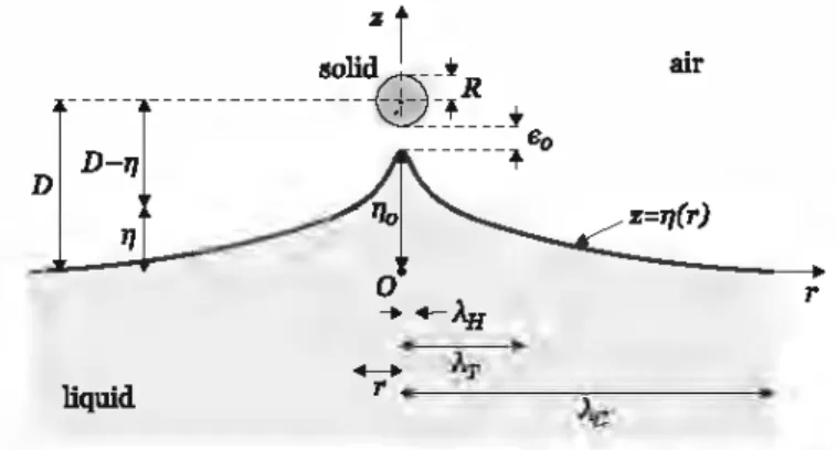
Considering that the London-van der Waals (London-vdW) interaction force between molecules acts over a rel-atively short distance, only the rounded extreme of the tip generates a reaction at the interface [9]. Consequent! y, in order to understand the nature of the noncontact interaction between a local probe and a deformable material surface, we model the tip as a sphere of radius R. Within a cylindrical coordinate system, a perfectly rigid sphere is placed at a fixed position over a serni-infinite liquid body, which is deformed like the one shown in Fig. 1, the gap between them being filled with air.

zj

solid {;"\ _

*

--- ---

ｂＭＭｾＭｾＭＭｙ＠ D-J'I ---ＭＭｾ＠ eo D air z=q(r) r liquid

FIG. 1. Scheme of the liquid surface deformation in interaction with a probe. Parameters defined in the text.

The interface is initially fiat and located at z = O. Based on the Hamaker theory [10], the pressure field (or attractive potential)

n

exerted by the sphere at a distance D over the bulk liquid is

4HR3 ₁

ll =

ｾ＠

[(D-z'fl +r2-R2]3' (1)

where H is the Hamaker constant of the probelairlliquid system, while z and r are the vertical and the radial

co-ordi.n.ates of any point in the liquid, as shown in Fig. 1. Equation (1) is obtained from integrating the London-vdW interaction potential between the sphere atoms and a

differ-entiai. volume at a given distance from the sphere surface.

As shown in Fig. 2, the radial cxtent of the pressure field

is smaller than the spbere radius. As

well.

consîdering the dilated vertical axis, which allows the visualization of the corresponding equilibrium liquid surface, the depth barely

0.04 0

ｾ＠

til ..().04 -0.08 -().12 0 1 -2 3HR.3 II/4H 10 20 30 40 50 60 70 Ｑｾ＠ ｾＱ＠ sphere diameter -1 0 2

r/R

FIG. 2. Pressure field over the liquid body generated by the interaction with the spherical probe, obcained from Eq. (1), and the corresponding interface deformed position for H = 4 x 10-2D Nm and R

=

to-

1 _{m. The vertical axis is m.agnificd to facilitate the}

interface visual recognition.

reaches 0.1 times the sphere radius. In brief, the interaction

effect is restricted to a very small zone over the liquid phase.

In tum, this attractive potential tends to deform the interface, which provokes a capillary pressure difference and a hydrostatic pressure in order to balance the system, as weil as a dynamic contribution entailed by the viscous dissipation of the system. As a first approach, we have disregarded the inertia1

effect with respect to the viscous contribution. Thence, the

genera1ized Young-Laplace's equation without mass transfer,

which describes the interface behavior, is expressed as

rr -

!l.pgJ7 +!!.. E . !!. = 2Ky, (2)

where !ip is the density difference between the liquid phase

and the air, g is the gravitational acceleration. !!. • :E • !!. is the normal viscous stress difference across the interface characterized by the unit normal vector !!_, " is the local

interface mean curvature, y is the surface tension, and '1 is the local interface position, which within an axisymmetric mode1 is given as a function of the radial position r and the time t.

Within this portrayal, inertia was disregarded with respect to

viscous dissipation because, at the AFM scale, the Reynolds number is of the order of Re e [1

o-

9 _{,1 d'].}

Additionally, considering a general case for which large

deformations are envisaged, the expression of the curvature in

cylindrical coordinates is given by

Ｒｴ｣］ＭＡ｟Ａ｟｛ｲ｡ＧｾｻＨ｡ＧｾＩＲ＠

_r

_{ar ar ar}

+1}-'J.

(3)

As well, in the more simplistic case, the viscous stresses at the air-side are negligible with respect to those at the liquid-side. Hence, for an incompressible single-directional viscous flow, which moves mainly in ｴｨ･ｾ＠ direction, and considering that

in cylindrical coordinates!!. is approximated by

nr

ｾ＠ -a7j

jar

and nl ｾ＠ 1, we have

a

(a11)

2

n · :E ·n ｾ＠ _,_

--

-

.-at

ar .

(4)

where IL represents the viscosity of the liquid. We can introduce

the definitions of the capillary length, l.c = .Jy /(Apg), and the relaxation time, l'

=

ＨｒｾＮｴＩｦｹＬ＠ of the system. As weil,

considering R as the characteristic length-scale and T as the

characteristic t:im&-scale of the system, we find the dimension-lesa variables: D• = D / R the distance from the center of the sphere to the originally undefonned interface, r• = r

1

R and

z•

=

z/

R the horizontal and vertical coordinates, 11* = 11/ R

and ｾ･Ｊ＠

=

"R the deformation and curvature, l.ê = l.c

1

R the

dimensionless capillary length, and t" = t f'r the dimension-less time. Thus, matching Eqs. (1)-{4), the nonlinear partial differentiai equation that describes the instantaneous position of the interface is written as the following dimensionless expression:

in which we find two dimensionless parameters: the Bond number B0

=

(R/Àci and the modified Ramaker number

Ha= 4Hj(3rryR2).

This dimensionless analysis gives rise to an equation that is valid for a system of any length-scale. In addition, as it is clearly observed from the parameter definitions, Ha and B0

are coupled by R. Renee, their values are restricted according

to the product of physical properties given by:

HaBo

=

3: ( H

::g).

(6)

Considering real probe/air/liquid systems [1 ,11- 13], for which HE [10-21,10-19]J, y E [lo-2,10-1_{]N/m, l:!..p E}

[102, 104]kgjm3, and IL E [10-3, 10°]Pa s, and common AFM probes, with R E [10-8, 10-7], the range of the

dimension-less parameters remains within Ha E [1

o-

8, 10-1] and B0 E

[10-11 , 10-8].

For simplicity, the deformation, and its first and sec-ond derivatives with respect to r* are written as TJÔ•

｛ｔｊＪ｝ｾＮ＠ and ｛ｔｊＪ｝ｾＮ＠ respectively, when evaluated at r*

=

0, and as TJè, ｛ｔｊＪ｝ｾＮ＠ and ｛ｔｊＪ｝ｾＮ＠ respectively, when evaluated atr*

=

Àê.

At r*

=

0, a symmetry boundary condition, ｛ｔｊＪ｝ｾ＠

=

0, should be considered. Meanwhile, far from the axis at

Àè

»

0, where the interaction potential, which decays as (r*r6_{, is} negligible (TI :::::i 0), the boundary condition cornes from the

quasistatic asymptotic solution ofEq. (5), also considering that in this outlying region the surface is nearly flat ([TJ*l'

«

1). The exact solution, which leads to the corresponding faraway boundary condition, is

TJ* = G Ko(

...[ii;

r*), (7)

with the coefficient G

=

TJè! Ko(1), and Ko being a zero-order

modified Bessel function of the second kind. Renee, the boundary condition at r* =

Àè

is given by

(8)

where K 1 is a first -order modified Bessel function of the second

kind.

We suppose that the interface is undeformed and completely flat before the dynarnic process starts. Renee, the initial condition at t

=

0, is given by TJ*

=

[TJ*l'

=

K*

=

0 for all

r* ｾ＠ 0, which is equivalent to say that the sphere is suddenly set at t =O.

After a time interval close to r, a steady-state profile is expected to be obtained. Considering real probe/air/liquid

systems, we find r E [10-6_,10-10_{]s for AFM situations.}

Because of the relatively small magnitude of this char-acteristic time-scale compared to the common laboratory measured time-scales, as a second approach, we consider that the steady state is reached instantaneously. At equilib-rium, liquid and interface are motionless, viscous stresses do not appear and the temporal derivative in Eq. (5) is ornitted. Thus, Eq. (5) is transformed into a dimensionless nonlinear ordinary differentiai equation and, as expected, the equilibrium profile is obtained when the interaction pressure field is totally compensated by the gravity and the capillary contributions.

A posteriori, it was verified that ([TJ*l'i

«

1, which supports the employment of the small interface dis placements hypothesis in our theoretical analysis. Taking this into account, the dimensionless mean curvature K* is decomposed in two principal curvatures

2K*

=

ｋｾ＠

+

K: (9a)

* d2TJ* * 1 dT]*

K

= - -

K

= - - - ,

(9b)

m dr*2 a r* dr*

where ｋｾ＠ is the dimensionless meridional curvature-the axisymmetric curvature of the interface that determines the behavior of the profile at any axial plane-while

K;

is the dimensionless azimuthal curvature-the curvature projec-tion of the circle describing isodeformaprojec-tion contour lines in the direction normal to the interface.

B. Numerical method

Due to the impossibility of solving analytically the strongly nonlinear Eq. (5), a numerical method was implemented. Firstly, taking care of the singularity present at r*

=

0, we consider the Taylor expansion

1 d *

- _!!____ :::::i [TJ*]"

+

O(r*). (10)

r* dr* 0

Additionally, employing the finite difference method to dis-cretize the time derivative, we can write the dynarnic term as

a ( aTJ*

)2

1

1

(

aTJ*

)21n (

aTJ*

)21n-1 }

at* ar*

=

l:!..t* ar* - ar* ' (ll)

where n and n - 1 indicate two consecutive time-steps, and

l:!..t* is the dimensionless time-s tep of the simulation.

Now, writing Eq. (5) as a system of nonlinear ordinary differentiai equations, we have to solve

(12a)

where u is the fust spatial derivative of the liquid surface position, 11*

=

TJ*In for sirnplicity, and A

=

(dTJ* jdr*)2_1n-l is a numerical method parameter. The problem represented by Eqs. (12) must be solved to obtain the profile of the interface at any time n, with the knowledge of the profile at the

previous instant n - 1. This system is a two-point boundary

value problem, which is worked out using a MATLAB routine including the function bvp4c.m, which employs the so-called Sirnpson's method [14]. Because of the smooth shape of the composing functions of the system expressed in Eqs. (12), the solution is easily found with the proposed method.

The boundary and initial conditions are

r*

=

0 ::::} u=O (13a) r* ］￀ｾ＠ ::::} _{u = -}JB:Kt(1) * Ko(1) l'Je (13b) t

=

0

1

_::::}

{ ••

ｾ＠

•7(1-

;;l

ｾｾ＠ (13c) 0 ｾ＠ r* ｾ＠

Àc

u

=

ＭＩＮｾＧ＠

where

'17

is the initial guess of the interface apex position. Due to the nonlinearity of the system, two different shapes of the interface profile can be found as simultaneous solutions of Eq. (5), depending on the value of

'17

(this point is discussed in Sec. III C). For the dynamic calculation of the profile evolution, the surface is initially placed at

'17

=

O. For steady-state calculation, the dynamic system is transformed into the equivalent system of equations, which describes the static case. The previous and the current instants are then nullified, and we take A

=

u2 _{and suppress the superindex n.}

For ali the situations, dynamic or static, interface profiles are calculated with a relative tolerance of

w-

4•

DI. LIQUID SURFACE DEFORMATION A. Transient state

From the results presented in the literature [9], for a given combination of the parameters Ha and B0 , the evolution of the

interface profile depends completely on the relative value of

D*. If D* is greater than a threshold value, Drin, a bumplike equilibrium profile is attained. On the other band, if D* is smaller than Drin, the profile deformation grows until the liquid touches the sphere, developing the so-called jump-to-contact processes and the formation of a liquid capillary bridge [15].

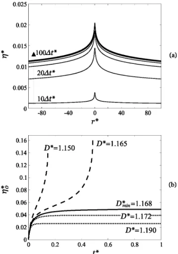
A typical interface profile evolving and reaching an equi-librium state is shown in Fig. 3(a). As well, the different evolution paths that the interface apex can follow, depending on D*, are shown in Fig. 3(b ). For ali the considered values of D*, the instantaneous application of the attractive force at t

=

0 directly results into an abrupt acceleration of the interface. In turn, surface tension generates a restoring force, which acts to oppose the interface deformation. As a consequence, the driving force in the next instant results from the balance between attractive and surface tension forces, both increasing along with the deformation. At the initial stage, the interface speed decreases monotonically due to the viscous dissipation within the liquid phase, which tends to damp the bulk liquid motion. If D* > Drin• the attractive force is sufficiently small to be controlled by the surface tension, and

*

::::-0.025 0.02 0.015 0.01 0.005 0 0.16 0.14 0.12 0.1 10Llt* -80 -40 D*=l.150 1 1 1 0 40 r* 1 D*=l.165 1 80 ｾ＠ 0.08 1 1 / 1 0.06 , ' , . ,. " ;

ｄｾ［ｮ］ｬＮｬＶＸ＠

ＰＮＰＴｾ＠ ｾ＠ ... D*= 1.172 .. .. 0.02 ｾ＠ ... ＧｪｪＮｾＺ￯Ｚ￯ＹＧＧＧ＠ ｯｾＭＭＭＭｾＭＭＭＭｾＭＭＭＭｾＭＭＭＭｾＭＭＭＭｾ＠ 0 0.2 0.4 0.6 0.8 t* (a) (b)

FIG. 3. Interface dynamic evolution obtained from solving Eqs. (12) for Ha= 10-3, Bo

=

10-10_{, and !:!.t*}

₌

_10-3_{• (a)}

Instan-taneous dimensionless profiles forD*

=

1.2 > Dri,, corresponding to increments of lO!:!.t* (from bottom to top). (b) Time-dependent dimensionless apex position for: [- -] D* < Dri,, [-] D*

=

Dri,, and[···] D* > Dri,.

the interface motion slows down until a steady-state profile is achieved, as represented by the dotted curves in Fig. 3(b ). The solid curve indicates the critical dynamic evolution, for which D* = Drin and the profile converges slowly toward an equilibrium state, attained near t* ｾ＠ 1. In contrast, when

D* < Drin• the attractive force is large enough togo beyond the tension force, and the motion grows without a regulating mechanism, leading to the sphere-liquid contact. The profile begins normally its deformation and the speed decreases until it reaches a temporary shrinkage, followed by arise of the speed, the profile divergence, and the subsequent wetting process. Also in Fig. 3(b ), the dashed curves describe this behavior, characterized by the so-called jump-to-contact process.

B. Steady-state equilibrium profile

The interface profile converges toward a final steady-state solution on1y if D* ｾ＠ Drin. An example of the typical equilibrium deformation profiles are shown in Fig. 4, for fixed values of Ha and B0 , and an initially flat surface placed at

'17

=

0, but for different values of D*. The corresponding curvatures,

K!

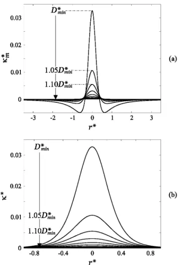
andK* [seeEq. (9)], aredisplayedinFig. 5. Asit

(a) (b)

0.05 0.04

*

s::::- 0.03 0.02

FIG. 4. (a) Steady-state dimensionless equilibrium profiles and (b) zoom of the central region obtained from solving the steady-state Eq. (5), for Ha = 10-3

, Bo = 10-10

, an initial guess with 117 = 0, and

D* with increments ｯｦＰＮＰＵｄｾ＠ (from top to bottom). In this case, it was found that ｄｾ＠ = 1.168.

is clearly depicted in the deformation profile shown in Fig. 4( a), the sphere pulls the interface towards itself only at a very reduced zone near the symmetry axis, as shown in Fig. 4(b ), which is a central region zoom. From r* ｾ＠ 102- 103 and

beyond, the asymptotic solution expressed in Eq. (7) perfectly describes the declining capillary behavior of the deformation. In addition, the meridional and mean curvatures are shown in Figs. S(a) and S(b), respectively. There is a passage from a negative to a positive value of

K:,,

near r*

=

0.37, which indicates a change in the sense of the surface tension force in the axial plane. On the contrary, K* remains always within positive values, showing a narrow logisticlike behavior, barely covering a projected radius. In short, from the curves in Figs. 4 and 5, reducing D* provokes an increment in the magnitude of the attractive force, leading to greater deformation and curvature states, as well as a slight variation of the radial extension of both.

C. Bifurcation diagrams

In fact, for each combination of the parameters Ha, B0 ,

and D*, two solutions for the deformation profile arise from the initial value chosen for TJ7. By taking D* and the two corresponding values of TJÔ as coordinate pairs, we obtain a bifurcation curve. Examples are shown in Fig. 6(a) for a fixed value B0

=

w-10_{• WhenD*}

₌

_{Drin, thereisonlyonesolution}

profile, corresponding to the maximum apex deformation ｔｊｾ＠

and the minimum gap

Erin

between the liquid surface and the sphere. There is no solution for the deformation profile further to the left than this critical point ＨｄｲｩｮＬｔｊｾ｡ｸＩＬ＠ from which the two branches emerge.

As observed from Fig. 6(a), the curve showing the highest apex deformation is thus an unstable branch from the energetic point of view. As well, the curve reporting the lowest apex position, associated to the minimum deformation energy, is a stable branch and thus describes the only possible interface profile. For the stable apex position, the dependency of TJÔ

on D* seems to take the form of a rectangular hyperbola:

*E: ｾ＠

*

ｾ＠ 0.03 0.02 (a) 0.01 0 -3 -2 -1 0 2 3 r* 0.03 0.02 (b) 0.01 Ｐｾｾｾｾｾｾｾｾｾｾ＠ -0.8 -0.4 0 0.4 0.8 r*

FIG. 5. Steady-state dimensionless equilibrium (a) meridional curvatures and (b) local mean curvatures obtained from solving the steady-state Eq. (5), with the same parameter values and variables as in Fig. 4.

the shorter the gap between the probe and the undeformed surface, the larger the deformation becomes. In Figs. 6(b) and 6( c ), the derivative of TJÔ with respect to D* and the curvature of the stable branch are shown, respectively. In both cases,

Drin marks the location of a vertical asymptote, at which the

stable branches are completely halted.

An increase of Ha generates a displacement of the

bifur-cation curve to larger values of D*, as well as a proportional scaling. Conversely, an increase of Bo provokes a very small

decrease of D*, which is negligible in comparison with those provoked by Ha. In general, the impact of Ha is significant, while the effects of a change in B0 are negligible within

the range of common liquids, as it is summarized in Fig. 7. Increasing Ha provokes an enlargement of ｔｊｾ＠ and Drin;

while, if B0 increases, both ｔｊｾ＠ and Drin show slightly smaller

values.

D. Geometrie relations

Noncontact AFM experiments require to control the tip/liquid distance, which is a function of their physical properties. This can be done by considering the geometrie relations that are presented below. When analyzing the apex

0.8 0.6

*0

_(a) 1::--0.4 0.2 0 0

*

ｾ＠

_*O

-2 (b)

..§"

-4 Ha (c) 1.2 1.4 1.6 1.8 2

D*

FIG. 6. Bifurcation diagrams: (a) apex deformation of the inter-face, (b) its derivative with respect to the separation distance, and ( c) its mean curvature, as functions of D*, for Ha E [1 o-s, 10-1]

and Bo = 10-10. Numerical solution of the steady-state Eq. (5) for

[ o] the stable and [ <>] the unstab1e branches, and the analytical solution for [-] the stable and [- -] the unstable branches given by Eqs. (14) and (15). In (a) the position of the sphere surface [·] is shown.

behavior for a given combination of Ha and B0 , it is found that

KÔ

grows along with TJÔ, which in turn becomes larger when

D* decreases, as observed in Fig. 8. The curvature

KÔ

shows a remarkable simple dependency on TJÔ, given by

(14) in which the prefactor C Rj 0.4(B2·06 / ｈｾﾷ Ｕ Ｉ＠ is obtained from

fitting the solutions of Eq. (5) for the range of parameters considered. From Fig. 8, a horizontallogarithmic displacement is produced when modifying the dimensionless numbers: significantly toward larger values of TJÔ when Ha increases; barely noticeable to smaller values of TJÔ when B0 grows.

While TJÔ moves towards TJ::rnx,

KÔ

reaches its maximum value

0.25 0.25 0.2 0.2 ｾ＠ 0.15 *E _0.1 0.15 !::"" ｾ＠ 0.05

-*E !::"" 0 0.1 10-11 10-10 10-9 10-8 (a) Ba 0.05 0 1.8 1.6 1.6 -5 *E 1.4 Cl 1.2 -5 ,. *E 1.4 Cl 1 10-11 10-10 10-9 10-8 (b) Ba 1.2 Ｑ ｇＭｾｾｾ ｾｾ ＭＭｾＭＭＭＭＭＭｾｾ＠ 10-8

FIG. 7. (a) Maximum apex deformation and (b) minimal dimen-sionless distance as functions of Ha for a fixed Bo = 10-10, and (insets) as functions of Bo for a fixed Ha= 10-3_{• [a] solution of the}

steady-state Eq. (5), and[-] tendency curve from the combination ofEqs. (16), (18), and (19).

K:UU.

Rj 3.3 x 10-2, whichstaysnearlyconstantforany Ha and

B0 • TJ::rnx and

K:UU.

indicate the limits ofvalidity ofEq. (14).

For the case of local probes, R is always much smaller than Àc, and as a consequence B0

«

1. Thence, the effect of

the capillarity is negligible compared to that of the attractive term at the symmetry axis, which corresponds to say that TJÔ is fully controlled by the London-vdW potential. Following this statement, disregarding the hydrostatic term in the steady-state Eq. (5), and analytically solving for D* at r*

=

0, we obtain

D*

=

TJÔ

+

1

₊

(Ha

)1/3

2 _Ko * ' (15)

which, when substituting Eq. (14), gives the dependency of

D* on TJÔ, leading to the bifurcation diagram's construction. The resulting relationship supplies the two physically possible solutions of Eq. (5), both stable and unstable branches. Bifurcation curves obtained using Eqs. (15) and (14) are also shown in Fig. 6(a), corresponding to a fixed B0 = 10-10 and

a range Ha E [1

o-

8, 10-1]. Furthermore, the derivative of TJÔ

with respect to D*, as well as

KÔ,

are compared to the stable branch results in Figs. 6(b) and 6( c ), respectively. In a11 cases, a very good accordance with the numerical solution is observed.

10°

w-2

10-4 *0 ｾ＠

w-6

w-s

FIG. 8. Apex mean curvature

Ko

as a function of T/Ô obtained for different modified Hamaker numbers in the range Ha E [1 o-8, 10-1]

and a fixed Bond number of Bo = 10-10 _{and (inset) for different Bond}

numbers in the range B0 E

[10-11_{, IQ-}8_{] and a fixed Ha = IQ-}3_{• [- ·-]}

indicates 1/:;.ax obtained from the evaluation in Eq. (14) of

1/::.U.

in turn obtained when solving Eq. (18). Arrows indicate the growth of the corresponding parameter.

From Fig. 1, the separation distance D between the liquid surface and the probe center, and the height of the interface apex 1Jo are related by an evident geometrie relation

ｄＪ］ｬＫｲｊｾＫｅｾＬ＠ (16)

where ｅｾ＠ = Eo/ R is the dimensionless gap between the deformed interface and the sphere surface. Combining Eq. (16) with Eq. (15) gives the exact expression of the dimensionless gap

(

H

)1/3

ｅｾ＠

= 1

+

₂

KJ

-

1, (17)

which, once more with the employment of Eq. (14), also relates ｅｾ＠ and rJÔ. Considering that the apex position diverges

at Drin, thus ､ｲｊｾｦ､ｄＪ＠ --+ oo, we obtain Drin by calculating

analytically the minimum of Eq. (15). Combining the latter with Eq. (14), the acquired polynomial

* 3

(

Ha * 512 1 Ha

Ｉ

ｾ＠

(

Ｉｾ＠

(rJmax)

+

2C (rJmax) - 16 2C

=

O, (18) is meant to be solved in order to find the maximum deforma-tion, and used to determine the minimum separation distance and the corresponding gap. The minimum gap is now given by

Erin=

1

+

(Ha)l/3_1_ -1

2C ｾ＠ ' (19)

while Drin is obtained when substituting ＱＱｾ＠ and

Erin

in Eq. (16).

In conclusion, the employment of Eq. (14) leads to find expressions, with which we can easily determine Ｑ｝ｾＬ＠

Erin,

and Drin. Together with the knowledge of Ha and B0 , which

are determined using data from the literature [1,11 ,12] or ex-periments [9], the optimal AFM scanning separation distance

range ]Dmïn,2R] is found. Such information is important for imaging liquid topographies and material properties at the nanoscale.

Iv. DEFORMATION SCALING

A. Characteristic length-scales

Taking

rr•

=

3:;rr R3_{ITj4H, wewritethesteady-stateEq. (5)} as follows:

(20)

The absolute value of the terms appearing in Eq. (20) and the curvature decomposition terms in Eq. (9), which contribute to achieve an equilibrium steady state, are depicted in Fig. 9. The existence of three important length-scales, already introduced in Fig. 1, is emphasized.

Firstly, corresponding to the position for which

K:;.

=

0

(inflection point of the meridional profile), ￀ｾ＠ indicates the boundary of a near-field zone, and the beginning of a transition zone, where ali the variables contribute to the deformation. At r* E [O,ÀM, the attractive term HaiT* (positive) is mostly opposed by 2K* (positive), whereas the hydrostatic term B01J*

(positive) is negligible. Characterized by Ha, the equilibrium profile in this near-field range is directly controlled by the balance between attractive potential and capillary pressure, both showing constant magnitudes that slowly decay when r* ＭＭＫ￀ｾＮ＠

Then, at the radial extent for which 2K*

=

0 (zero-curvature), À} marks the end of the transition region and

10°

ｾ］］］］ｾ

ｾＭＭｾｾＭＭｾｾＭＭｾｾ＠

10-5 (a) ｾ＠ 1 -10 -...:.. 0 ••••••••••••••••••••••••••••••••••oo•ooo oomm""""""•--... ' , F ' \ T 10-15 _N

'

10-20

ｾ＠ ｾ＠

ｾ＠

10°

_...

10-5 K* _K* m a

B:

10-10 (b) 10-15 _{N T F} 10-20 10-2 100 102 104 106 r*

FIG. 9. Characteristic length-scales determination. Different terms (a) xj from Eq. (20), for which

L:

xj

=

o,

and (b) Yj from Eq. (9), for which

L

yj = 2K*, as functions of r*' for Ha =

w-

3'

B0 = IQ-10_{,andD* = D::Un = 1.168. TheuppercaselettersN, T,and}

F designate the near-field, transition, and far-field zones, respectively, which extents are bounded by the characteristic length-scales ￀ｾＬ＠ ￀ｾＬ＠

1.6

ＧＧ ｾ＠

1.2 1.2 _{ｾＺｴＺＰＮＸ＠} Ba

*:ti

...;;: 0.4 ［Ｂｾ＠ (a) 0.8 0 o 0.05 0.1 0.4 _Ｑ｝ｾ＠ 0

ｍ ｾ＠

60 6o B ... 0

*"'

40

ｾ＠

::

1

(b) ...;;: 20 0 o 0.05 0.1 Ｑ｝ｾ＠ 0 0 0.05 0.1 0.15 0.2 0.25 0.3 Ｑ｝ｾ＠

FIG. 10. (a) Radial position of the inflection point of the profile

￀ｾ＠ and (b) radial position of zero-curvature ￀ｾＬ＠ as functions of ｦｩｾＬ＠

with the same parameter values and variables as in Fig. 8, as well as the same considerations for the insets. Arrows indicate the growth of the corresponding parameter.

the beginning of the far-field zone, which corresponds to a capillarity dominated decay. When r* ｅ｝￀ｾＬ￀ｽＨＬ＠ K; with-stands both Ha II*, which quickly loses its intensity, and

K;;,,

which has adopted a negative value. In this region,

K;;,

and

K;,

the latter al ways showing a positive value, are

antagonists. B0TJ* remains nearly constant as it slowly gains

weight while both Haii* and 2K* decrease at the same rate.

Finally, the dimensionless capillary length

Àc

shows the extension at which the effect of all terms tend to disappear. Within r* E]À},Àè], Hai1* has become negligible whereas

2K*, which has become negative, attains the order of magnitude of B0TJ*. In this zone, B0TJ*, which diminishes gradually, is

opposed by 2K*, while K;;, and K; are still contending. The shape of the interface profile in this far-field zone is completely given by B0 • Beyond r*

=

Àc,

the interface returns to its

unperturbed fiat state.

In Fig. 10, ￀ｾ＠ and À} are shown as functions of TJÔ for different Ha and B0 • For a given combinations of parameters,

￀ｾ＠ and À} decline as functions of TJÔ, following rectangular hyperbolalike behaviors. This tendency continues until the values of ｄｾ＠ and ｔｊｾ｡ｸ＠ are reached, for which the limiting equilibrium profile and the minimum radial positions of ￀ｾ＠

and À} are attained. The numerical results indicate that

￀ｾ＠ shifts toward higher values when Ha increases in the range Ha E [10-8, 10-1 ]. On the other hand, the impact

of B0 on ￀ｾＬ＠ within B0 E

[10-11_{,10-8], is not significant.}

Likewise, À} follows the same tendency when Ha augments; however, we observe an important decrease of À} when Bo

grows.

The curves in Fig. 10 can also be analyzed as follows. For a given Ha, a decrease of D* provokes the growth of

0.8 *O _0.6 )< ;;;--._ (a) )< 0.4 0.2 0 -5 -4 -3 -2 -1 0 1 2 3 4 5

r*/ À'fi

N ₀ ｾ＠ ｾ＠

_•

*O

•

)<

•

•

ｾ＠ -1

_•

•

(b)

••

*0

_••

!::'"

_••

*1

•

!::'" -2 ' - ' -10 -8 -6 -4 -2 0 2 4 6 8 10

r*/À'fi

FIG. 11. Near-field self-similar dimensionless (a) curvature and (b)interfaceprofilefor Ha E [10-8,10-1] andB0 E [10-11,10-8]. [o] numerical solution of the steady-state Eq. (5) and [-] approximations obtained from Eqs. (21) and (23), for the curvature and the interface profile, respectively.

TI* and TJÔ, leading to a decrease in both ￀ｾ＠ and À}, which

is the action of the capillary pressure to restrain the radial extent of the deformation. From another viewpoint, an increase of Ha generates a given TJÔ at a larger D*, and both ￀ｾ＠

and À} are subsequently increased, which indicates that the attractive potential spans over a larger zone. Because D*

and its induced TJÔ are not significantly affected by B0 , a

change in this parameter has a faint effect over ￀ｾＮ＠ On the other hand, an increase of B0 directly provokes a decrease

of À}, which corresponds to enlarging the heaviness of the interface.

B. Self-similarity

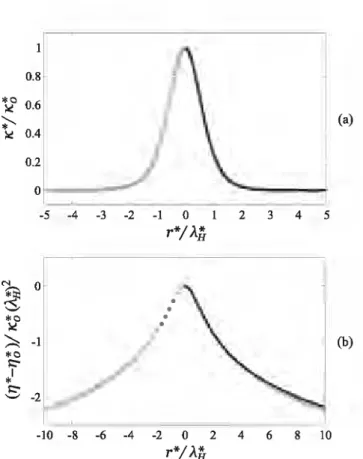
Taking into account the length-scales, ￀ｾ＠ and Àc, we find master curves that display the self-similarity of the deforma-tion profile in the near- and far-field zones, respectively. For

r* E ｛ｏＬ￀ｾ｛Ｌ＠ the reduced variables K* /KÔ and r* Ｏ￀ｾ＠ allow us to find the dimensionless curvature presented in Fig. 11(a). This curve exhibits a logisticlike probability function shape

4exp

{-br;.)

H ₍₂₁₎

[1 +exp{-

br;. )]2'

H

where b is a fitting parameter, which is deterrnined below.

The relative error between the numerical solution of K* /KÔ

In addition, the reduced curvature K* / KÔ can be tak:en as negligible for radial positions beyond r* Rj 1 Ob ￀ｾＮ＠

Matching Eq. (21) with Eq. (3), for small displacements of the liquid surface, and integrating we find

_..!:_ dTJ* - 8K*(b

￀ｾＩ＠

{ exp ( -

ｾＩ＠

r* dr* - 0 r* 1 +exp ( -

br;. )

H +

Ｈ｢ｲＺｾＩＨｭ｛ＱＫ･ｸｰＨＭ

｢ｲ［ｾＩｊＭｲｮｂＩｽＮ＠

0 N -2 ｾ＠

'$

_-4 *0 ;:,c )::: _-6 *0 !::" *1 -8 !::" ' - ' -10 -12 35 30 25 ｾ＠ 20

;;;-..

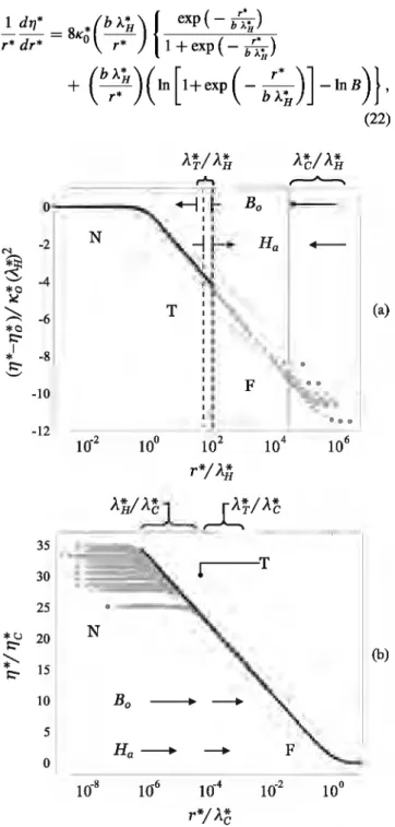
!::" 15 10 5 0 N 10-2 N À*/À* _{T H} rA-I 1.---'T Bo - ----+ 10-4 ｲＪＯ￀ｾ＠ À*/À* _{C H} ,---A--.. (22) (a) (b)

FIG. 12. Self-sunilar deformation profile obtained with the di-mensionless variables in (a) Eq. (23) and (b) Eq. (24). [o] numerical solution of the steady-state Eq. (5) and[-] approximations obtained from Eqs. (23) and (24). The uppercase letters N, T, and F designate the near-field, transition, and far-field zones, respectively. Vertical lines indicate the positions of the reduced characteristic length-scales, while the sense of the arrows shows its displacement when the corresponding dimensionless parameter grows: shifting Ha E

[10-8_,10-1

] for a fixed Bo

= 10-

10 , and varying BoE [10-11,10-8]

for Ha = 10-3_•

where B is an integration constant. From the boundary conditions ｛ｔｊＪ｝ｾ＠ = 0 and the corresponding Taylor expansion of the logarithmic term, we find B = 2. As well, evaluating Eq. (22) and (21) atr* ］￀ｾＬ＠ where 2K* = K;, wededucethe value of b = 3.89 x 10-1. Afterward, performing a second integration of Eq. (22), we obtain the expression of the dimensionless deformation profile

TJ*- TJo _{* *}

2{

1 [ ( r* )] 2 =8b -ln- 1+exp - - b * Ko(ÀH) 2 ÀH

1

r• f(b >.;,.) 1 dx } + ln -[1 +exp (-x)]- , 0 2 x (23) where x is an integration variable. Once more, the relative error

between the numerical solution and Eq. (23) is also 10-3_{, for a}

radial position up tor* ｾ＠ Ｕ￀ｾＮ＠ In Fig. ll(b), the self-similar profile given by Eq. (23) is compared to the numerical results, showing a very good agreement within 0 ｾ＠ r* ｾ＠ ￀ｾＮ＠ for Ha E [10-8_,10-1_{] and B}

0 E

[10-11_{,10-8 ]. Therefore, it is proven}

that (TJ*-ｔｊｯＩＯｋￔＨ￀ｾＩ Ｒ＠ _{and r* Ｏ￀ｾ＠ are the dimensionless}

variables that characterize the self-similar behavior of the deformation in the near-field zone. The logarithmic plot of these parameters, depicted in Fig. 12(a), exposes that this self-similarity spans largely over the transition zone.

Forr* ｅ｝￀ｾＬ￀￪｝Ｌ＠ thecoupleofreduced variables TJ* !TJê and

r* /Àê, where TJê = TJ*(r* = Àê), leads us to find the far-field self-similar deformation profile

KoG:) _c

Ko(1) ' (24)

As shawn in Fig. 12(b), Eq. (24) gives a quite good de-scription of the far-field results within ￀ｾ＠ < r* ｾ＠ Àê, and even spanning over the whole transition zone. The decaying behavior, described by the far-field self-similarity, is observed for r* ｅ｝￀ｾＬｯｯ｛Ｎ＠

V. CONCLUDING REMARKS

An extensive anal y sis of the deformation of a liquid surface, due to its interaction with a nanoprobe, was presented. The phenomenon was portrayed by a strongly nonlinear equation, and the effects of physical and geometrie parameters over the system were considered. Mainly when the interaction within a nanoscale system is considered, our madel generates a more accurate description of the interface deformation than previous works [16,17], which employ the Derjaguin approximation. Furthermore, the application of our results is possible at any scale, considering realistic situations, due to the performed dimensionless approach.

The interface profile evolution, whether the system attains equilibrium or not, depends on the relative magnitude of D*

with respect to the threshold distance

v::nn.

which in tum is given by the combination of the remaining parameters, B0 and

Ha. Bifurcation diagrams relating TJo and D* are established,

in which a zone with nonexistent equilibrium is uncovered and explained, when D* <

n::nn.

On the other band, steady-state stable and unstable equilibrium profiles are obtained when

D* ｾ＠

v::nn.

thus the attractive force is thwarted mostly by the

Three different length-scales were obtained from the analysis of the steady-state equilibrium profiles, all of them being function of Ha and/or B0 • They determine the existence

of: a near-field zone, r* E [O,ÀM, controlled by the attractive interaction/surface tension balance; a far-field zone, r* E

｝ＩＮＮｽＬＩＮＮｾ｝Ｌ＠ dominated by the gravity/surface tension interplay; and a transition zone, r* E]À1J,À}[, where all the variables take an important role. It was found that the two interior length-scales are affected by the size of the probe: ÀH

;S

R

and Àr ｾ＠ lOR, while the capillary length remains fixed Àc "' 10-3. These length-scales are responsible for the liquid surface self-similar deformation profile.

[1] J. N. lsraelachvili, Intermolecular and Surface Forces, 3rd ed. (Elsevier, Amsterdam, 2011 ).

[2] E. Pelletier, J. P. Montfort, and F. Lapique, J. Rheol. 38, 18 (1994).

[3] J. N. Sharpe, Handbook of Experimental Solid Mechanics (Springer, Berlin, 2008).

[4] A. Knoll, R. Magerle, and G. Krausch, Macromolecules 34, 4159 (2001).

[5] H. J. Butt, B. Cappella, and M. Kappl, Surf. Sei. Rep. 59, 1 (2005).

[6] T.-D. Li andE. Riedo, Phys. Rev. Lett. 100, 106102 (2008). [7] M. Delmas, M. Monthioux, and T. Ondarcuhu, Phys. Rev. Lett.

106, 136102 (2011).

[8] B. A. Todd and S. J. Eppell, Langmuir 20, 4892 (2004).

The curvature of the stable profile is found to take a remarkable shape at its apex, ｋｾ＠ ex ＨＱＷｾＩ ＳＯＲ ＠ This fact and the problem geometry give rise to accurate simple formulas for computing the minimum separation distance ｄｾＬ＠ its corresponding maximum deformation IJmax and minimum gap ｅｾＬ＠ when Ha and B0 are previously known [1,11,12]

or experimentally obtained [9]. The knowledge of ｄｾ＠ is fundamental when searching the optimal scanning noncontact AFM conditions, in order to avoid undesired capillarity effects. Nevertheless, the power-law relationship between ｋｾ＠ and ＱＷｾ＠

remains a factual but empiric result, which is a topic for future studies.

[9] R. Ledesma-Alonso, D. Legendre, and P. Tordjeman, Phys. Rev. Lett. 108, 106104 (2012).

[10] H. C. Hamaker, Physica 4, 1058 (1937).

[11] L. Bergstrom, Adv. Colloid Interface Sei. 70, 125 (1997). [12] J. Visser, Adv. Colloid Interface Sei. 3, 331 (1972). [13] K. Mougin and H. Haidara, Europhys. Lett. 61, 660 (2003). [14] L. F. Shampine, 1. Gladwell, and S. Thompson, Solving ODEs

with MATLAB (Cambridge University Press, Cambridge, 2003). [15] F.M. Orr, L. E. Scriven, and A. P. Rivas, J. Fluid Mech. 67, 723

(1975).

[16] F. P.-A. Cortat and S. J. Miklavcic, Langmuir 20, 3208 (2004).

[17] Y. Z. Wang, D. Wu, X. M. Xiong, and J. X. Zhang, Langmuir 23, 12119 (2007).