Multiplexing Avionics and additional flows on a QoS-aware AFDX network

HAL Id: hal-02970656

https://hal.archives-ouvertes.fr/hal-02970656

Submitted on 19 Oct 2020

HAL is a multi-disciplinary open access

archive for the deposit and dissemination of

sci-entific research documents, whether they are

pub-lished or not. The documents may come from

teaching and research institutions in France or

abroad, or from public or private research centers.

L’archive ouverte pluridisciplinaire HAL, est

destinée au dépôt et à la diffusion de documents

scientifiques de niveau recherche, publiés ou non,

émanant des établissements d’enseignement et de

recherche français ou étrangers, des laboratoires

publics ou privés.

Multiplexing Avionics and additional flows on a

QoS-aware AFDX network

Oana Andreea Hotescu, Katia Jaffrès-Runser, Jean-Luc Scharbarg, Christian

Fraboul

To cite this version:

Oana Andreea Hotescu, Katia Jaffrès-Runser, Jean-Luc Scharbarg, Christian Fraboul. Multiplexing

Avionics and additional flows on a QoS-aware AFDX network. 24th IEEE International Conference on

Emerging Technologies and Factory Automation (ETFA 2019), Sep 2019, Zaragoza, Spain. pp.282-289,

�10.1109/ETFA.2019.8869506�. �hal-02970656�

Multiplexing Avionics and additional flows on a

QoS-aware AFDX network

Oana Hotescu, Katia Jaffrès-Runser, Jean-Luc Scharbarg, Christian Fraboul

Institut de Recherche en Informatique de Toulouse, Université de Toulouse, INPT-ENSEEIHT, 2 rue Charles Camichel, 31300 Toulouse, France

Email: {oana.hotescu, kjr, jean-luc.scharbarg, christian.fraboul}@enseeiht.fr

Abstract—AFDX is the standard switched Ethernet solution for the transmission of avionics flows. Today’s AFDX deployments in commercial aircrafts are lightly loaded to ensure the determinism of control and command operations. Manufacturers envision to take advantage of the remaining AFDX bandwidth to transmit additional non avionics flows (video, audio, service). These flows must not compromise the in-time transmission of avionics ones: constraints on jitter at source end system and end-to-end latency have to be insured for each avionics flow. In this paper, we investigate the scheduling of avionics and additional flows, mainly at the end system level. We show that an event-triggered strategy is better than a time-triggered one for additional flows at source level, but it might compromise the jitter constraint of avionics flows and increase the end-to-end latency of additional ones. We consider two time-triggered scheduling strategies, i.e. an optimal one and a simpler one based on a heuristic. We show that the later one performs nearly as well as the former one and that, for both of them, the difference with an event-triggered strategy at source level is limited and can be statically bounded.

I. INTRODUCTION

The drastic increase of embedded systems and avionics functions in civil avionics has led, at the turn of the century, to the design of the now de-facto networking standard named AFDX [1] (Avionics Full-DupleX switched Ethernet). This standard offers a deterministic networking service to a large amount of control and command flows. These flows are carried using virtual links (VL) whose bandwidth is preserved using traffic policing at the network entrance. This policing is possible since all flows are generated with a maximum jitter by the source end system.

Several approaches have been proposed to upper bound end-to-end delays, including network calculus and trajectory approach [3], [2]. The bound on the end-to-end delay provided by these methods is shown to be relatively pessimistic in [4], resulting into a lightly loaded network [3].

Therefore manufacturers envision the network to be shared by regular control command avionics flows and less critical video, audio or service flows related to aircraft monitoring and maintenance operations. Therefore, it is of course mandatory to guarantee that delay as well as jitter constraints are still satisfied for avionics flows. Moreover, if video or audio flows are considered, their timely streaming at the destination is only possible if appropriate guarantees on their end-to-end delay are offered. Thus, advanced scheduling mechanisms have to be implemented both at the switch and end system levels.

At the switch egress ports, Static Priority Queuing (SPQ) scheduling policy with 2 priority levels is currently deployed. It is suitable for the case where a single type of additional flows is carried by the network. Adding more types of flows necessitates the use of advanced scheduling policies such as Deficit Round Robin (DRR) or Weighted Round Robin (WRR). In this paper, we focus on a single type of additional flows.

At source end system, avionics flows have to be regulated as to ensure the fact that they don’t use more bandwidth than planned. This regulation requires the jitter at end system output to be upper bounded to a value specified by the standard (typically 500 µs). The scheduling policy implemented in end systems has to guarantee that this constraint is not violated. This paper investigates different candidate scheduling policies for end systems.

To the best of our knowledge, no previous work has been dedicated to the optimization of source scheduling for different levels of QoS in an AFDX network. Work has been dedicated in the last years to the problem of finding an optimal schedul-ing schema in synchronous time-triggered networks, such as TTEthernet [5], [6], [7] and TSN [8]. The main originality of our problem is related to the impossible synchronization of AFDX end systems and switches. Thus, an event-triggered strategy has to be used at switch level.

The main contribution of the paper is to propose and compare event-triggered as well as time-triggered strategies for the scheduling of mixed flows at source end system.

Section II presents the AFDX network with avionics and additional flows. Section III details the proposed scheduling strategies for end systems. These strategies are compared on a realistic case study in Sections IV and V. Section VI gives conclusions and directions for future works.

II. PROBLEM STATEMENT A. The AFDX network

Avionics Full DupleX switched Ethernet(AFDX) [1] is a switched Ethernet-based network that has been designed for safety-critical avionics applications. An AFDX network is composed of a set of end systems interconnected by switches and physical links. Each end system is connected to a single switch port by a unique physical link. Data exchange between end systems can occur only through virtual communication channels called Virtual Links (VLs). A VL connects one

source end system to one or more destination ones. VLs share the network bandwidth. Thus, each virtual link is assigned an upper bounded bandwidth specified by a Bandwidth Allocation Gap (BAG) and a maximum frame size Smax. The BAG represents the minimum time interval between two consecutive frames transmitted through the VL. The BAG value is given in the set of powers of 2: {1, 2, 4, 8, 16, 32, 64, 128} milliseconds. For a given VL, at most one frame of maximum allowed size can be transmitted within a BAG duration.

A subset of an AFDX configuration is depicted in Figure 1. Six VLs v1 . . . v6 are shown. They are transmitted between five end systems through seven switches. Black dashed lines represent sets of links to/from end systems and switches which are not represented in Figure 1. Additional flow a1 will be explained in Section II-B. Table I summarizes VL features.

sw3 sw4 sw6 sw5 sw1 es1 sw7 sw2 v1,v4,v6 v1,v4,v6 v2,v5 v2,v5 v1,v2,v3,v4,v5 es2 v6 v3 v4,v6 v1 es3 es4 es5 v2 a1 (additionnal flow) v5 v4,v5,v6 v1,v3

Fig. 1. Illustrative AFDX configuration

VLs in Figure 1 have identical frame size (500 bytes), leading to a transmission time of 40 µs at 100 Mb/s. In this paper, we

TABLE I

ILLUSTRATIVE CONFIGURATION FLOWS

Type BAG/period (µs) Smax(bytes)

v1 Av 4000 500 v2 Av 16000 500 v3 Av 2000 500 v4 Av 128000 500 v5 Av 1000 500 v6 Av 2000 500 a1 Add 80 500

assume A350-like AFDX configurations. Such a configuration is composed of two redundant networks interconnecting 126 end systems across 14 switches. 1106 VLs are transmitted on this network.

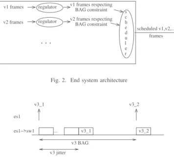
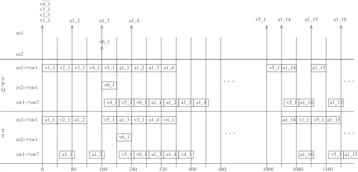
At end system, the BAG constraint has to be guaranteed for each VL. As depicted in Figure 2 a traffic regulator is associated to each VL. It delays any frame which does not respect the BAG constraint. Then, frames coming from the regulators are multiplexed by the scheduler into a single flow to be sent on the output physical link. If multiple frames from different VLs arrive at scheduler input at the same time, some of them may experience queuing delay or jitter. Figure 3 illustrates this jitter on VL v3 in figure 1. The transmissions of two consecutive v3 frames are shown. The first one is delayed by competing frames at the output port of es1, while the second one is transmitted immediately. Therefore, these two frames arrive at switch sw1 within an interval which is smaller than the BAG, i.e. BAG− jitter where jitter is the waiting time of the first frame in es1. This jitter can be problematic.

Indeed the network doesn’t trust the end system. Thus, the BAG constraint of each VL is checked at the entrance of the network. The distance between two consecutive frames of a given VL should never be less than the BAG minus the maximum possible jitter for this VL. The ARINC 664 P7-1 standard specifies that the jitter for a given VL must not exceed 500 µs. s c h e d u l e r v1 frames respecting BAG constraint regulator v1 frames regulator

. . .

Fig. 2. End system architecture

v3_1 es1 es1−>sw1 v3_1 v3_2 v3_2 ... v3 BAG v3 jitter

Fig. 3. Jitter at end system

At the switch level, there are two FIFO queues (high priority, low priority) at each output port. Each incoming frame is buffered in the queue corresponding to its priority. Classically, frames are served in each output port, following a static priority queuing (SPQ) policy (high priority first). Up to now, all VLs are assigned the high priority level.

B. Additional flows on the AFDX network

The AFDX network has to be certified. Typically, a proof of determinism has to be provided: safe upper bounds have to be provided on frame end-to-end delays. Several methods have been proposed to compute such upper bounds, e.g. network calculus [9], [11], trajectory approach [10], forward end-to-end delay analysis (FA) [12]. These methods have to take into account very rare worst-case scenarios and they are based on pessimistic assumptions, resulting in a lightly loaded network. Typically, link load in a 100 Mbps AFDX configuration exceeds 10 % for a very small subset of the links and it never exceeds 25 % [3]. A similar situation occurs for the A350, even if the load is slightly higher since fewer switches are in use. Thus the avionics industry envisions to use the available AFDX bandwidth for the transmission of additional flows of lower criticality such as video, audio or service data flows. Currently, these flows are carried by dedicated communication networks, introducing additional weight and maintenance costs. The goal is to remove these dedicated networks and integrate all flows on the core AFDX backbone.

It is of course mandatory to guarantee that delay as well as jitter constraints are still satisfied for avionics flows. Moreover, if video or audio flows are considered, their timely streaming at the destination is only possible if appropriate guarantees on their end-to-end delay are offered. Thus, advanced scheduling mechanisms have to be implemented both at switch and end system levels.

As previously mentioned, a single type of additional flow is assumed in this paper. Therefore, the already implemented SPQ 2-priority levels is used at switch egress port. In the next section, we describe candidate scheduling policies at the end system level.

III. SCHEDULING AT THE END SYSTEM LEVEL

Figure 2 gives an overview of the architecture of existing end systems. As previously mentioned, regulators ensure that each VL respects its bandwidth limit. A scheduler multiplexes frames from the different VLs on the output link.

Additional video and audio flows are regulated, while ser-vice flows might not be regulated. Usually, video flows have higher demand of transmission than audio flows or avionics flows, but they are not authorized to exceed the available bandwidth. Nevertheless, these additional flows have to be scheduled with the avionics VLs. For avionics flows, the main constraint is the maximum allowed jitter at source end system, i.e. 500 µs as specified in the ARINC 664 standard. In the next paragraphs, we present the two classes of solutions for the scheduling of frames at end system level:

• the event-triggered solutions where pending frames are transmitted, based on their arrival time and priority order, • the time-triggered solutions where pending frames are

transmitted in dedicated slots.

A. Event-triggered scheduling

In an event-triggered scheduling, pending frames are se-lected for transmission, based on their priority and the cor-responding scheduling policy. Many scheduling policies have been considered, such as FIFO, SPQ, WRR or DRR. In the context of this paper, we assume two types of flows: critical avionics flows and less/not critical additional ones. The impact of additional flows on avionics ones has to be strictly mastered. Thus FIFO scheduling policy cannot be considered, since avionics flows would be delayed by a potentially large number of additional frames (all pending frames at the arrival of the avionics one).

The other scheduling policies are able to control the impact of additional flows on avionics ones. With WRR or DRR, a guaranteed portion of the bandwidth is allocated to each class of flows, leading to an isolation between classes. The portion of bandwidth is the number of frames for WRR and the number of bytes for DRR. Considering SPQ scheduling policy, the impact of additional flows on avionics ones can be limited to one frame with maximum size provided that avionics flows have a higher priority than additional ones. Since existing AFDX hardware implement SPQ with two priority levels and

we address one single type of additional flows, we assume such a scheduling policy in the context of this paper.

Figure 4 considers the flows emitted by end systems es1 and es2 in Figure 1. The SPQ part in Figure 4 shows a possible scenario when SPQ scheduling policy is implemented at the end system level. At time 0, one frame from each VL v1, v2, v3, v4, v5 and from additional flow a1 is ready at end system es1. Based on SPQ, VLs have a higher priority than additional flow. Thus, frames from the VLs are transmitted first, in an arbitrary order (v11, v21, v31, v41, v51 in Figure 4). Then frames from additional flow a1 are transmitted (a11 arrived at 0 and the following ones arrived later). At time 1000 µs, v5 second frame is ready for transmission (v5 BAG is 1 ms) and it is immediately transmitted, since there are no other pending frames in es1.

As previously mentioned, SPQ scheduling policy is used in switch output ports. Thus, VL frames are transmitted in their arrival order, while additional frames are transmitted in their arrival order, provided there are no pending VL frames.

In the scenario in Figure 4, additional frames have no impact on VL ones. The situation might be different if an additional frame is under transmission at the arrival time of a VL one. However, this impact is bounded by the transmission duration of one additional frame. Thus it can be easily taken into account.

Let’s now consider the jitter of VLs at the end system level. In Figure 4, v5 is the only VL with two transmitted frames, since it is the only one with a BAG smaller than 2 ms. The first frame of v5 waits till time 160 µs, since there are four other pending VL frames which are arbitrarily transmitted first (they are ready at the same time). Conversely, the second one is transmitted immediately (at time 1000 µs). Thus, the jitter for v5 at its source end system is 160 µs in this scenario. Using such an SPS scheduling, this jitter might increase dramatically when the number of VLs generated by the end system increases. As previously mentioned, this jitter must never exceed 500 µs.

One goal of the time-triggered scheduling presented in the next paragraph is to mitigate this jitter.

B. Time-triggered scheduling

In an AFDX network without additional flows, Time-triggered scheduling can be implemented in end systems by statically reserving slots for each VL [13]. It comes to build a table as the one depicted in Figure 5 for es1 in Figure 1. The duration of each slot should be at least the transmission time of any frame in the configuration. In Figure 1, the transmission time of any frame is 40 µs. Thus the slot length in Figure 5 is 40 µs. The scheduling in the table is repeated forever. Therefore the duration of the table is the least common multiple of the BAGs, i.e. 128 ms. In Figure 5, one line duration is 1 ms, leading to a table with 128 lines. The four first lines are represented. v5 is allocated one slot every line, since its BAG is 1 ms. Following the same principle, v3 is allocated one slot every two lines.

es2

v6_1

v5_1 v6_1

v2_1 v5_1

a1_1 a1_2 a1_3 v3_1 a1_4 v4_1

v6_1

a1_1 a1_2 a1_4 v4_1

a1_1 v5_1 v4_1 v3_1 v2_1 v1_1 0

v4_1 v5_1 v6_1 a1_1 a1_2 a1_3 a1_4 v6_1

es2−>sw1

v1_1 v2_1 v3_1 v4_1 a1_1 a1_2 a1_3 a1_4 v5_1

v1_1 a1_3 v5_1 v5_1 v5_1 v5_1 es1

a1_2 a1_3 a1_4

80 sw1−>sw7 es1−>sw1 es2−>sw1 sw1−>sw7 es1−>sw1 S P Q T T a1_14 a1_14 a1_14 a1_15 a1_15 a1_15 a1_15 1000 160 240 320 400 480 1080 1160

. . .

. . .

v5_1 a1_14 a1_15 a1_16

a1_14

. . .

. . .

Fig. 4. Scheduling at the end system level

v2 v5 v3 v4 v1 v5 v5 v3 ... ... ... ... ... ... ... ... 40 us 1000 us

Fig. 5. Table with one slot per BAG per VL

Considering the table in Figure 5 and the scenario in the upper part in Figure 4, we obtain frame transmission as depicted in the TT part in Figure 4 (we assume that the table starts at time 0).

Since the duration between two consecutive slots allocated to a given VL is exactly a BAG, the duration between two consecutive transmissions of a given VL is never less than its BAG (although it can be more since the BAG is a minimum inter-frame duration). Thus, the jitter constraint is guaranteed by construction for each VL: the upper bound of the jitter is 0.

The main drawback of this time-triggered solution is the waiting time till the next slot allocated to the VL, which can be close to the BAG. In Figure 4, this waiting time is more than 1 ms for VL v1. Depending on the scenario, it could be close to 128 ms for v4.

A classical solution to mitigate this problem is to over-reserve slots: for instance, if one slot is allocate to each VL every ms, a frame will never wait more than 1 ms. Thanks to the regulator unit associated to each VL in its source end system (Figure 2), a VL will never use more than one slot

within a BAG. In the rest of the paper, we assume such an over-reservation (one slot per ms per VL). It comes to assign one column of the table to each VL. This over-reservation limits the available bandwidth for additional flows. Therefore, a compromise between the over-reservation and the waiting delay till the next slot might be an interesting solution for VLs. This point is left for future work.

When additional flows are considered, their impact on avionics one has to be mastered. The simplest solution is to schedule these additional flows in the free slots of the table. This solution is illustrated in the TT part in Figure 4. Pending additional frames have to wait till the next free slot(s). Obviously the positions of the VL slots in the table will impact this waiting time. In the next paragraphs, we propose two policies for the assignment of slots to VLs in the table.

1) Uniform table scheduling: The idea of the first policy is to uniformly distribute free slots in the table. It is based on a very simple heuristic. Columns of slots assigned to VLs are spread in the table so that the distance between any two columns is the same. Figure 6 shows such a table for es1 in Figure 1. Since we have 5 VLs and 25 slots per ms, one column is allocated to a VL every 5 slots (columns 1, 6, 11, 16 and 21). v1 v1 v1 ... ... ... ... ... ... v2 v2 v2 v3 v3 v3 v4 v4 v4 v5 v5 v5

2) Optimal table scheduling: The second policy aims at choosing the slot assignment of VLs that minimizes the emis-sion lag of additional flows, i.e. the maximum waiting time of any additional frame in the end system. The problem can be formulated as an integer constrained optimization problem. The two types of flows are defined by the following sets:

• A set V of VLs with for which a bounded jitter has to be ensured. These flows need an entire column reservation in table scheduling in order to keep their jitter to zero. • A set A of additional flows whose maximal emission lag

has to be minimized.

The following definitions are given: • D_srepresents the slot duration.

• N represents the number of slots composing the table. • P_Ai is the actual period of frame generation for an

additional flow Ai∈ A.

• N_A is the number of frames generated by all additional flows in A during the table duration.

• |V | is the number of avionics VLs in V • L is the number of lines in the table • C is the number of columns in the table

Two different types of decision variables are defined: • the integer decision variables{xi}i∈[1,NA] that take their

values in the integer set{1, .., N }. xi gives the identifier of the slot where an additional frame i is scheduled. Thus, x= [x1, .., xi, .., xNA] is a sorted set of slot identifiers. • the integer decision variables {yj}j∈[1,|V |] representing

the slot at which the first avionics frame of VL Vj is scheduled. Following frames of Vj are scheduled period-ically every line of the table. These variables take their values in the integer set {1, .., C}.

There is one variable yj for each VL and one variable xi for each additional frame.

The additional frames generation dates are listed in the ordered set {di}i∈[1,..,NA]. The value of di represents the

slot number in which the frame i is generated and thus di∈ {1, .., N }.

The optimization criterion minimizes the maximum emis-sion lag over all additional frames. The emisemis-sion lag is given by δi= xi−direpresenting the number of entire slots between the generation and the actual scheduling date of an additional frame i.

The following mathematical program is defined: M inimize max i∈[1,..,NA] (xi− di) Subject to: xi> xj, i > j, ∀i, j ∈ [1, NA] (1) xi≥ di, ∀i ∈ [1, NA] (2) xi6= yj+ (l − 1)×C, ∀i ∈ [1, NA], ∀j ∈ [1, |V |], ∀l ∈ [1, L] yj 6= yk, j6= k, ∀j, k ∈ [1, |V |] (3) The set of constraints in equation (1) ensures that a slot in the scheduling table can be assigned to exactly one additional

frame while the set of constraints in equation (2) ensures that a slot can be assigned to an additional frame only after its frame generation date. Equation (3) ensures that a VL can be assigned slots in a single column of the table. The slots on this column can neither be assigned to another VL nor to an additional flow. The problem dimension is given by the number of VLs and the number of frames generated by the additional flows.

IV. CASE STUDY A. Network configuration

Currently deployed AFDX networks work at 100 Mbps. To be able to carry additional flows such as video or audio data, network data rate needs to be increased. For this reason, aircraft manufacturers envision to increase AFDX data rate to 1 Gbps in future deployments.

In our case study hereafter, we consider 1 Gbps AFDX network carrying additional uncompressed video flows coming from surveillance cameras situated on various locations of the plane.

The video transmission in avionics systems follows the ADVB standard specifications [14]. It specifies that only

uncompressed digital video streams can be exchanged in the avionics systems to mitigate stream reconstruction delays at the receiver. This protocol is based on Fiber Channel Audio Video (FC-AV) protocol which is particularly suited for high bandwidth communications of high-resolution video streams. The delivery of video data without compression is needed by the avionics systems supporting time-critical functions such as assisted takeoff and landing, navigation, etc. Thus, neither frame losses nor additional latency introduced by compression/decompression operations are tolerated.

A video is composed of a sequence of images referred to as video frames. A video frame is transmitted as a sequence of data packets called ADVB frames. The sequence of ADVB frames form an ADVB container that is specific to a single video frame. ADVB frames are labeled with an object field that represents the type of data carried in the frame:

• Object 0 frame contains video frame header data (image information and auxiliary data),

• Object 1 frame contains audio data, • Object 2 or 3 frames contain video data.

For the transmission of an image, the first frame is of object 0 type and lists information related to the image (sequence num-ber, type of color coding, dimensions, etc.). ADVB standard specifies that, to encapsulate video data into frames, images are scanned from left to right, line by line. If the last frame’s payload for a line is not complete, padding bytes are added to keep the frame size constant.

The ADVB frame is very similar to the frame used for Eth-ernet with a maximum frame length of 1518 bytes including 1500 bytes of payload. Therefore, AFDX network is a good candidate to deliver video streams in accordance with ADVB specifications.

ADVB specifies several video formats. These formats are listed in Table II. In this paper, we consider VGA and XGA

formats. XGA video format with 3-byte color requires a resolution of 1024 pixels× 768 lines per image, progressively scanned from left to right and from top to bottom as 3-byte RGB pixels. This format needs 3072 bytes per line that can be encapsulated into 3 Ethernet frames. To encapsulate the entire image, a total of 2305 frames will be used (2304 frames for the video data and 1 additional frame for the auxiliary information). A video that displays 24 frames per second has to receive 55320 frames per second with a bandwidth requirement of 640.685 Mbps. Since video is uncompressed here, the period of video frame generation equals 18.076µs for XGA format. Similarly, the VGA format with 640 pixels × 480 lines per image leads to a bandwidth requirement of 280 Mbps and a period of Ethernet frame generation of 43.35µs.

TABLE II

ETHERNET FRAME ENCAPSULATION FOR DIFFERENT VIDEO DISPLAY FORMATS IN3-BYTESRGBAND FRAME SIZE OF1518BYTES.

Display format Data rate Period Number of (pixels×pixels) (Mbps) (µs) video frames/s QVGA(320 × 240) 93 129.8 7 704

VGA(640 × 480) 280 43.35 23 064 SVGA(800 × 600) 350 34.69 28 824 XGA(1024 × 768) 672 18.076 55 320 SXGA(1280 × 1024) 896 13.55 73 752

The network configuration is similar to the one deployed on the Airbus A350 on which a couple of ADVB video flows are added. The basic configuration is composed of 126 ES, 7 switches on each redundant network and 1106 VLs. A unique ES of this configuration is subject to video transmission. This ES is source of 8 VLs emitting frames periodically at their BAG. BAG values of these VLs are in the set of {4, 8, 16, 32} as indicated in Table III. The maximum frame length of avionics frames carried by these VLs is between 115 and 835 bytes.

TABLE III

VLS AT SOURCEESTARGETED FOR VIDEO TRANSMISSION

VL 1 2 3 4 5 6 7 8

BAG(ms) 16 16 8 32 4 4 32 16 Length 131 579 323 115 323 115 835 131

Paths of these VLs cross from 1 to 3 switches. Video flows can be added on any of these paths. The most loaded switch egress port uses around 40 Mbps of the 1Gbps available on the network. The rest of the bandwidth can thus be dedicated to video flows. Thus, video flows originating from the same ES cannot exceed 960 Mbps.

We illustrate here two possible scenarios for the evaluation. • First, one camera is deployed. A single XGA video flow (768 × 1024) with a requirement of 672 Mbps can be transported into the network.

• Second, two cameras are connected to the given ES for redundancy. The screen resolution needs to be decreased making possible the transmission of 2 SVGA flows with a requirement of 350 Mbps each or of 2 VGA flows requiring each 280 Mbps.

Next we discuss the scheduling of these additional video flows at the end system level.

B. Scheduling at end system

We now focus on the source ES and we analyze how the scheduling policy impacts the transmission of video flows.

1) Event-triggered: If SPQ policy is applied at ES level, no bandwidth over provision is required. The total amount of available network (approximately 994 Mbps) can thus be used by the video flows. Therefore, the three scenarios of video transmission established previously are possible(i.e. 1 XGA, 2 SVGA or 2 VGA flows).

2) Time-triggered: The table scheduling is configured with 1Gbps data rate. The table is composed of 128 lines of 1ms. Each line is divided into 64 slots of 15.625µs. This slot duration has been chosen as a function of the maximum frame length of the flows and the data link rate and it is long enough to transmit one frame of any flow. According to this time division, the table can be now represented as a 2D matrix of 128 lines× 64 columns.

When the order of frames is established at ES by the table scheduling, the number of time slots are over provisioned for avionics frames. Also, the slot duration of 15.625 µs is over sized so that a frame with the maximum length can be transmitted in a single slot. The total amount of bandwidth required for slot reservation of the 8 VLs is thus of 315 Mbps.The rest of the available bandwidth of 685 Mbps can be used by the video flows. In this case, only two scenarios of video transmission are still possible without exceeding the network bandwidth: 1 XGA video flow or 2 VGA video flows together with the VLs.

Uniform and optimal table schedules can be applied. Uni-form heuristic gives an emission lag of 1 slot to the XGA video flow and of 2 slots for the 2 VGA flows. The VLs distribution in the table corresponding to the columns allocated to them is the following one: {0, 8, 16, 24, 32, 40, 48, 56}. It is the same for the two scenarios of video transmission.

The mathematical optimization program is solved using the CPLEX commercial constraint solver [15]. The optimal table schedule produces the same maximum emission lag as the uniform one: 1 slot for the XGA flow and 2 slots for the 2 VGA flows. The solving time is around 1 hour and 20 minutes for both scenarios. However, the solutions are different as the VLs distributions in table are different. The VLs are allocated at columns {2, 10, 18, 26, 34, 42, 50, 58} for the transmission of the XGA flow. When 2 VGA are added, the VLs are assigned to columns in the set of {4, 11, 22, 29, 41, 46, 54, 62}.

These table allocations will be compared in Section V. V. END-TO-END DELAY EVALUATION

In this section, we evaluate the impact of scheduling strate-gies on VL and video flow delays. First, we give simulation results to evaluate the distribution of video flow delays for both event-triggered and time-triggered scheduling. Second we compute worst-case end-to-end latencies for VLs in order to

TABLE IV

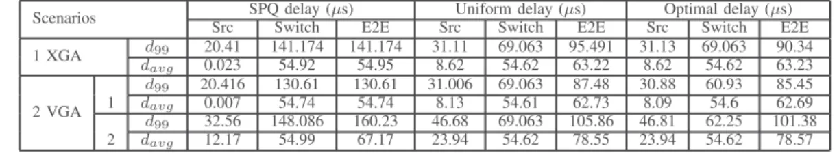
AVERAGE(davg)AND99TH CENTILE(d99)DELAYS FOR VIDEO FLOWS WITH THESPQ, UNIFORM ANDOPTIMAL TABLE SCHEDULES. SCENARIOS CONSIDER8 VLS SHARING THE BANDWIDTH WITHi) 1 XGAFLOW ANDii) 2 VGAFLOWS. END-TO-END(E2E)DELAY IS COMPOSED OF SOURCE,

SWITCH QUEUING AND LINK TRANSMISSION DELAY.

Scenarios _Src SPQ delay (µs)_{Switch E2E Src}Uniform delay (µs)_{Switch E2E Src}Optimal delay (µs)_{Switch E2E} 1 XGA d99 20.41 141.174 141.174 31.11 69.063 95.491 31.13 69.063 90.34 davg 0.023 54.92 54.95 8.62 54.62 63.22 8.62 54.62 63.23 2 VGA 1 d99 20.416 130.61 130.61 31.006 69.063 87.48 30.88 60.93 85.45 davg 0.007 54.74 54.74 8.13 54.61 62.73 8.09 54.6 62.69 2 d99 32.56 148.086 160.23 46.68 69.063 105.86 46.81 62.25 101.38 davg 12.17 54.99 67.17 23.94 54.62 78.55 23.94 54.62 78.57

determine the impact of video flows on VL worst-case delay. Such a worst-case analysis is mandatory for certification.

A. Simulation study

This section investigates the distribution of source, network and end-to-end delay of video and avionics frames for the event-triggered and time-triggered scheduling policies intro-duced previously in this paper. Next, our simulation settings are introduced. In a second stage, results for two representative scenarios are given and analyzed.

1) Simulation settings:

a) Simulator: Following results were produced by an in-house AFDX network simulator whose core relies on the OMNeT++ discrete event framework [16]. Our simulator models the main parameters of AFDX (routing of virtual links, queuing policies, switching latency, etc.). The simulation sce-nario considers the network architecture described previously. On these architecture, the video flows follow the path of the additional flow in Fig. 1.

b) Scheduling policies: At the switch level, a 2-level SPQ policy is applied. The higher priority is allocated to VLs and the lower one to video flows. At source ES, the delay statistics are compared for the SPQ policy and the uniform and optimal table schedules.

c) Network settings: The network data rate is set to 1 Gbps and the switching delay to 2µs. The results presented herein are made available for the case where the video flows and avionics VLs follow the same path and cross 3 switches. Thus, for a maximum frame size, the minimum expected end-to-end delay is 54.576 µs.

d) Offsets: There is no global synchronization of ADFX network pieces of equipment. Thus any possible shift is possible between any two end system, depending on their relative starting time and clock drift. We introduce random relative offsets in our simulations to capture this unpredictable shift. Indeed we have to take into consideration that not all end systems start emitting frames simultaneously and we define therefore an end system relative offset of end system X as the delay between the transmission date of the first frame in the network and the date of the first frame transmission by end system X. The sole assumption we make on these offsets is that they cannot exceed the maximum BAG value.

To capture the delay distribution of a wide range of possible scenarios, Monte-Carlo simulations are performed here. The relative offsets of end systems take a new randomly chosen

value in the [0..128ms] interval at each new simulation. Source, network and end-to-end delays of video frames are measured for each new simulation. All values are merged to obtain the global distribution of these delays. Repeated simulations have shown that around one hundred simulation runs are enough to retrieve a complete distribution.

e) Simulation duration: The simulation duration has been set to 384ms, corresponding to 3 × 128 ms. It is equivalent to 2 times the duration of the hyper period (128 ms) in addition to the maximum offset value of 128ms. This duration captures the complete delay distribution as after at most two cycles, the system behavior becomes cyclic. Since the end system offset is a random value, it will vary for each simulation run, leading to a variation of the number of generated frames during the same simulation duration. For that reason, we consider the distribution delay for the first 5906 frames arrived at their destination for the VGA display format and the first 14162 frames arrived at their destination for the XGA format.

2) Results: Results in Table IV shows the 99th centile(d99) and the average(davg) delay of video flows measured at source ES output, at network, and at destination ES with SPQ, Uniform and Optimal table schedules. The investigated scenarios consider the emission of i) 1 XGA video flow and ii) 2 VGA video flows together with 8 VLs.

The source delay experienced by the XGA flow is around 20.41µs with the SPQ policy and around 31µs with both uniform and optimal tables. As expected, delays with Uniform and Optimal table schedules are similar. The SPQ low delay value is due to the small number of VLs and the reduced length of avionics frames requiring a transmission delay between 0.92 to 6.6µs. Even though, the table scheduling produces a greater source delay because of the fixed time slot duration of 15.625µs, it is beneficial for avionics frames whose jitter is 0, while SPQ generates some delay variation due to the simultaneous emission of the VLs. Table schedule has a positive impact on the network crossing delay and on the end-to-end delay that are significantly reduced in comparison with SPQ.

Similar results can be observed on the 2VGA flows. These simulation results show that event-triggered policy can have a better performance for video flows at ES level, but it introduces a delay variation for VLs. Time-triggered policy may be disadvantageous for video flows at source ES, but null

jitter is ensured for avionics frames as well as a reduction of the end-to-end delay of video flows.

B. Worst-case analysis for avionics frames

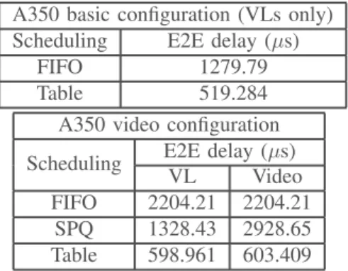
Table V shows the worst-case end-to-end delay for a VL crossing the same path as a video flow. Results have been com-puted first for the basic A350 network configuration where no video transmission is enabled. The case of a video flow added on this architecture is considered in a second stage. FIFO, SPQ and table scheduling applied at ES are compared. Worst-case analysis is realized with Network Calculus. Following results were produced with the C++ tool developed by A. Soni et al. in [17] implementing the latest version of Network Calculus.

TABLE V

WORST-CASE BOUND ON THE END-TO-END DELAY FOR AVLAND VIDEO FLOW CROSSING THE SAME PATH.

A350 basic configuration (VLs only) Scheduling E2E delay (µs)

FIFO 1279.79

Table 519.284

A350 video configuration Scheduling E2E delay (µs)

VL Video

FIFO 2204.21 2204.21 SPQ 1328.43 2928.65 Table 598.961 603.409

For the basic configuration, the worst-case end-to-end delay of the VL is higher with FIFO policy applied at ES level than with table scheduling. The upper bound on the end-to-end delay is reduced with table scheduling as offsets are introduced between VLs at source end system permitting to spread their arrival at the switch level. When a video flow is added, we can see that FIFO produces a large upper bound delay on both VL and video flow as no priority is considered between flows. SPQ allows the use of two priorities reducing the bound on the VL’s end-to-end delay. This bound is clearly reduced with table scheduling. Still, the impact on the end-to-end delay of the VL is limited in comparison with the basic video-free configuration.

VI. CONCLUSION

In this paper, we consider an AFDX network shared be-tween avionics and additional (less critical) flows. We inves-tigated event-triggered and time-triggered scheduling policies for the transmission of avionics and additional flows at the end system level. We show that an event-triggered strategy is better for additional flows at source level, but it might dramatically increase the jitter for avionics flows at source level and increase the end-to-end latency of additional flows. Therefore, a time-triggered strategy is the most promising candidate. We also show that a very simple heuristic can efficiently build such a time-triggered scheduling.

In this paper we assume a single type of additional flows. However, different types of additional flows are envisioned

by manufacturers. Thus our work has to be extended, first at the switch level where more complex scheduling policies should be considered (such as WRR or DRR), second at the end system level where types of additional flows should be treated differently.

REFERENCES

[1] Aeronautical Radio Inc. ARINC specification 664 P7-1, Aircraft Data

Network, Part 7: Avionics Full Duplex Switched Ethernet (AFDX) Network, 2009.

[2] H. Bauer, J. L. Scharbarg, and C. Fraboul, Applying and optimizing

trajectory approach for performance evaluation of AFDX avionics network, IEEE Emerging Technologies and Factory Automation (ETFA), 2009.

[3] H. Charara, J. L. Scharbarg, J. Ermont and C. Fraboul. Methods for

bounding end-to-end delays on an AFDX network, Proceedings of the 18th Euromicro Conference on real-time Systems (ECRTS’06), Dresden, 2006.

[4] H. Bauer, J. L. Scharbarg, and C. Fraboul. Worst-case end-to-end delay

analysis of an avionics AFDX network, Proceedings of the Conference on Design, Automation and Test in Europe, European Design and Automation Association, 2010.

[5] D. T˘ama¸s–Selicean, P. Pop, and W. Steiner, Design optimization of

TTEthernet-based distributed real-time systems, real-time Systems 51.1, pp 1-35, 2015.

[6] S. S. Craciunas, R. S. Oliver, and V. Ecker, Optimal static scheduling

of real-time tasks on distributed time-triggered networked systems, IEE Emerging Technology and Factory Automation (ETFA), pp. 1-8, 2014. [7] S. S. Craciunas, and R. S. Oliver, Combined task-and network-level

scheduling for distributed time-triggered systems, Real-Time Systems 52, no. 2, pp. 161-200, 2016.

[8] S. S. Craciunas, R. S. Oliver, M. Chmelík, and W. Steiner, Scheduling

real-time communication in IEEE 802.1 Qbv time sensitive networks, In Proceedings of the 24th International Conference on Real-Time Networks and Systems, ACM, pp. 183-192, 2016.

[9] J. Y. Le Boudec, and P. Thiran, Network calculus: a theory of

deter-ministic queuing systems for the internet, Springer Science & Business Media, vol. 2050, 2001.

[10] H. Bauer, J. L. Scharbarg, and C. Fraboul. Applying Trajectory approach

with static priority queuing for improving the use of available AFDX resources, real-time systems 48.1, pp 101-133, 2012.

[11] X. Li, J. L. Scharbarg, and C. Fraboul, Improving end-to-end delay

upper bounds on an AFDX network by integrating offsets in worst-case analysis, IEEE Emerging Technologies and Factory Automation (ETFA), 2010.

[12] N. Benammar, F. Ridouard, H. Bauer, and P. Richard, Forward

End-to-End Delay for AFDX Networks, IEEE Transactions on Industrial Informatics, 14.3, pp 858-65, 2018.

[13] O. Hotescu, K. Jaffrès-Runser, J. L. Scharbarg, and C. Fraboul, Towards

Quality of Service Provision with Avionics Full Duplex Switching, ECRTS 2017 Work-in-Progress Session, pp 19-21, 2017.

[14] ARINC specification 818-2 Avionics Digital Video Bus (ADVB) High

Data Rate, 2013.

[15] IBM ILOG CPLEX Optimization Studio CP Optimizer User’s

Man-ual. [Online]. Available:https://www.ibm.com/support/knowledgecenter/ SSSA5P_12.6.1/ilog.odms.studio.help/pdf/usr/CPoptimizer.pdf [16] A. Varga and R. Hornig. An overview of the OMNeT++ simulation

environment. In Proceedings of Simutools ’08. ICST, Brussels, Belgium, 2008.

[17] A. Soni, X. Li , J.L. Scharbarg and C. Fraboul, Work in progress paper:

pessimism analysis of network calculus approach on AFDX networks, 12th IEEE International Symposium on Industrial Embedded Systems (SIES), pp. 1-4, 2017.