HAL Id: hal-00201063
https://hal.archives-ouvertes.fr/hal-00201063
Submitted on 22 Dec 2007HAL is a multi-disciplinary open access archive for the deposit and dissemination of sci-entific research documents, whether they are pub-lished or not. The documents may come from teaching and research institutions in France or abroad, or from public or private research centers.
L’archive ouverte pluridisciplinaire HAL, est destinée au dépôt et à la diffusion de documents scientifiques de niveau recherche, publiés ou non, émanant des établissements d’enseignement et de recherche français ou étrangers, des laboratoires publics ou privés.
Numerical simulation of colloid dead-end filtration:
effect of membrane characteristics and operating
conditions on matter accumulation
Yolaine Bessiere, David Fletcher, Patrice Bacchin
To cite this version:
Yolaine Bessiere, David Fletcher, Patrice Bacchin. Numerical simulation of colloid dead-end filtration: effect of membrane characteristics and operating conditions on matter accumulation. Journal of Membrane Science, Elsevier, 2008, 313 (1-2), pp.52. �10.1016/j.memsci.2007.12.064�. �hal-00201063�
Numerical simulation of colloid dead-end filtration: effect of
membrane characteristics and operating conditions on matter
accumulation
BESSIERE Yolainea, FLETCHER David Fb, BACCHIN Patricea
aLaboratoire de Génie Chimique, Université Paul Sabatier, 31062 Toulouse cedex 9 – France bSchool of Chemical and Biomolecular Engineering , University of Sydney, NSW 2006, Australia
bacchin@chimie.ups-tlse.fr
Abstract
The aim of this work is to develop a simulation capability applicable to dead-end filtration of colloidal dispersions in order to investigate the effect of process conditions, such as membrane configuration and operating parameters, on filtration efficiency through the analysis of the appearance of a deposit on the membrane. To reach this goal, a model describing the transport behaviour of a concentrated colloidal dispersion is implemented in a commercial CFD code (ANSYS-CFX). The collective diffusion induced by inter-particle interactions is accounted for from knowledge of the variation of the osmotic pressure with the particle volume fraction. Coupled with a transient, two dimensional hydrodynamic solution, such a model allows description of the mass transport properties both in the dispersed (concentration polarization) and the condensed (deposit) forms of accumulation. Two-dimensional concentration profiles along the membrane are obtained. Simulations are used to understand the role of operating parameters and membrane characteristics on the appearance of a deposit at the
membrane surface. This formation is controlled by the hollow fibre configuration, where there are zones working in both cross-flow and dead-end mode due to the particular hydrodynamic conditions.
Key-words: CFD Simulation - Colloid - Fouling - Ultrafiltration – Aggregation – Heterogeneity
Nomenclature Roman
D diffusion coefficient (m2.s-1) H(φ) Happel function (-)
J filtration flux (m.s-1) mp particle mass fraction (-)
p pressure (Pa)
Rd hydraulic resistance induced by deposit formation (m-1)
Rm membrane permeability (m-1)
r radial coordinate (m)
rp particle radius (m)
t time (s)
U velocity vector (m.s-1)
Vacc volume of depositaccumulated per unit membrane area (m3.m-2)
Vp particle volume (m3)
Greek
α specific resistance of deposit (m.kg-1) ρ density (kg.m-3)
П osmotic pressure (Pa)
φ volume fraction (-)
μ dynamic viscosity (Pa.s)
τ stress tensor (Pa)
Subscripts b bulk
cp close packing
p particle s solvent
solid solid produced by deposit w water
1. Introduction
Colloidal fouling is always a severe problem to be faced when using membranes to separate particles from water in drinking or waste water processes [1]. To control the colloidal fouling it is necessary to understand the effects of specific colloid properties (mainly controlled by their surface interaction) on the matter accumulation at the membrane surface. It has been shown that with colloids, the deposit formation is the direct consequence of significant concentration polarization, which leads to a phase transition of the matter from a dispersed to a condensed state [2], this phase transition being linked to inter-particle surface interactions. The consequences of the transition have been theoretically and experimentally analysed in terms of critical fouling conditions both in cross-flow [3] and dead-end mode [4].
Furthermore, the effect of the membrane configuration is not well understood: in drinking water treatment hollow fibres are used more and more as they yield an efficient packing density allowing the civil engineering costs to be reduced significantly [5]. However, no study reports the impact of the hollow fibre configuration on the way colloids accumulate and a deposit appears at the membrane surface. It is linked to the fact that experiments analysing the deposit formation (and its possible heterogeneity along the membrane) are very hard to perform in in/out hollow fiber configuration. Light deflection techniques, ultrasonic reflectometry or magnetic resonance imaging techniques allows in-situ quantification of the fouling layer but do not provide enough detailed information below 100 micrometers [17].
Several questions remain: what is the effect of channel diameter on fouling? Does the low tangential velocity induced by the permeate flow play a role in the dead-end hollow fibre configuration? What are the consequences on the way deposit forms at the membrane?
To answer, at least partly these questions, this work aims to develop a model of mass and momentum transfer in dead-end filtration (i.e. time-dependant conditions) with an applied constant flux, in order to understand specific colloidal fouling behaviour associated with the hollow fibre configuration. After a short presentation of the state of knowledge of colloidal fouling and its description, the suspension properties and the assumptions used for the simulation of mass and momentum transfer are presented. Simulation results are then discussed by considering the dynamics of matter accumulation and identifying the position along the membrane where the transition between concentration polarisation and deposit formation is likely to occur.
2. Background
This study focuses on fouling controlled by surface mechanisms, i.e. concentration polarisation and deposit formation for which different models can be found in the literature. After a brief analysis of the phenomena involved in colloidal fouling, the existing classical filtration laws are presented in order to underline their limitations. 2.1 Colloidal fouling
Numerous studies have shown that fouling layers created during filtration of colloidal dispersion can exhibit both characteristics of concentration polarisation and deposit mechanisms [6]. The interplay between these mechanisms has been analysed through the existence of a phase transition [7, 8] in the colloidal dispersion which is linked to a
critical concentration in colloids. Through this analysis, the deposit formation can be seen as the consequence of a concentration polarisation mechanism which leads to the critical concentration at the membrane; the deposit formation is then preceded by a concentration polarisation mechanism. This concept of phase transition has been applied in membrane science to determine critical filtration conditions leading to the formation of deposit in tangential [9] and dead-end mode [10]. In dead-end filtration it has been shown, both from an experimental and theoretical point of view [4], that the interaction of concentration polarisation and deposit formation mechanisms has consequences on the accumulated layer reversibility and subsequently on the way filtration should be run to increase the productivity.
2.2 Modelling of filtration dynamics
To describe the evolution of permeability with time during dead-end filtration, it is generally assumed that the accumulated matter is homogeneous on the whole membrane surface. The variation of the accumulated volume of matter per unit area of membrane with time is then given for constant flux conditions by the following relationship:
t J
Vacc = φb (1)
When deposit formation is the main fouling mechanisms [11], it is classically assumed that the deposit is created on the membrane as soon as filtration begins. The additional hydraulic resistance induced by deposit formation, Rd, is then:
acc solid
d V
R =αρ (2)
where α is the specific resistance of the deposit and ρsolid is the density of the solid produced by the deposit formation. When operating at constant flux, such a model leads to a linear increase of the trans-membrane pressure with time that is classically used to
determine the specific resistance. However, such a modelling procedure of filtration is based on some assumptions:
• homogeneous accumulation on the membrane surface; • instantaneous deposit formation.
The validity of these assumptions is examined in this paper using 2D simulation of colloids filtration in tubular and hollow fibre geometries.
3. Model development
3.1 Modelling of colloidal properties
The description of the concentrated colloidal suspension is based on the variation of the osmotic pressure with the particle volume fraction, which is an experimentally accessible parameter used in colloidal science to account for multi-body particle interactions. To illustrate this, simulations are made using experimental data for the osmotic pressure corresponding to 40 nm radius (mean value by number, rp) latex
particles in 10-3 M KCl [3,12]. The colloidal osmotic pressure (or more precisely the variation of the osmotic pressure with particle volume fraction) has been theoretically shown as being useful to predict collective diffusion of particles in a concentration gradient and phase transitions between fluid (dispersed) and solid (condensed) phases occurring in a dispersion [7]. The details of this modelling approach are described elsewhere [12].
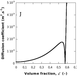
The collective diffusion coefficient can be estimated through the generalised Stokes-Einstein relation, where the diffusivity (D) is given as a function of the derivative of the
osmotic pressure (Π) with the volume fraction (φ), the radius (rp) and the volume (Vp) of
particles, the solvent viscosity (µs) and the Happel function (H(φ)) accounting for the
effect of concentration: φ φ πμ φ d d ) ( H 6 1 ) ( = p Π p s V r D (3)
The osmotic pressure and the diffusion coefficient variations with the particle volume fraction are given in Figures 1a and 1b, respectively. In this system of stable colloids, the presence of repulsive surface interactions between particles is responsible for an increase in both the osmotic pressure and the diffusion coefficient. As implied by theory, the transition between a fluid and a solid phase (i.e. when attractive interactions overcome repulsive interactions) is represented by the zero derivative of the osmotic pressure variation (Fig. 1a) and by a zero diffusion coefficient (Fig. 1b). This volume fraction dependence of the diffusion coefficient is implemented in the conservation equation for particle mass solved by the CFD code in order to account for this colloidal behaviour.
3.2 The computational model
Whilst there have been a large number of CFD studies performed to examine the flow in membrane channels and systems, there have apparently been no studies that combine the complex physics of colloidal behaviour in the wall region with flow modelling. Ghidossi et al. provide a recent review of CFD modelling across the entire domain of membranes [13] and demonstrate how CFD can be used in the study of a hollow fibre ultrafiltration system [14]. Wiley and Fletcher [15] developed a detailed CFD model of Reverse Osmosis that included feed and permeate channels, linked by detailed
modelling of the trans-membrane mass transfer process, and subsequently applied this to RO treatment of brackish water [16]. The computational approach developed here is based on that work but includes the addition of detailed modelling of the variation of physical properties based on the particle volume fraction.
The computational model reported here has been developed using ANSYS-CFX11 (http://www.ansys.com/cfx).
Geometry
Dead-end filtration with time-dependent flow of a latex dispersion in a tubular configuration (Fig. 2) is studied. The membrane is 1.3 m in length, comprising a 0.1m non-porous entry length (shown in grey in the figure) in order for the flow to have a fully-developed hydrodynamic boundary layer when it reaches the porous part. This hollow fibre has a standard lumen diameter of 0.94 mm (this parameter is investigated later) corresponding to a typical hollow fibre dimension and the fibre is closed at the end. To prevent an abrupt change in particle fraction at the end of the membrane the small length of impermeable wall was neglected and the membrane permeability was ramped down smoothly.
A two dimensional, axisymmetric slice of the tube (shown in red in Figure 2) was meshed with a structured mesh, generated using ANSYS ICEM-HEXA, having a very fine mesh near the membrane surface, with the nearest node located 0.15 microns away from the surface and the mesh expanded smoothly towards the fibre axis. Tests showed that this level of mesh resolution gave grid independent results.
The hollow fibre is fed with a 0.2 g.L-1 latex suspension (bulk volume fraction, φ
b =
1.4431×10⁻⁴) at fluxes ranging from 1.39×10⁻⁵ to 3.89×10⁻⁵ m.s-1 (50 to 140 L.h-1.m-2) corresponding to inlet velocities in the axial direction ranging between 0.071 to 0.199 m.s-1 when considering a 0.94 mm diameter hollow fibre. Considering an ultrafiltration membrane with low MWCO, the porous medium is, furthermore, assumed to be totally rejecting.
Formulation and solution of the conservation equations
Assuming an incompressible fluid and isothermal conditions, together with use of a mass-weighted velocity, the equations for the conservation of mass, momentum and particle mass are:
0 ) ( = ∇ + ∂ ∂ • ρU ρ t (4) τ U U U . ) ( ⊗ =−∇ +∇ ∇ + ∂ ∂ • p t ρ ρ (5) 0 ) .( ) ( −∇ ∇ = ∇ + ∂ ∂ • p p p m D m t m ρ ρ ρ U (6)
The stress tensor is given by ) . 3 2 ) ( ( U U δ U τ= μ ∇ + ∇ T − ∇ (7)
The fluid density, which is composition dependent, is given by ) / ) 1 ( / /( 1 mp ρp mp ρs ρ = + − (8)
where ρp and ρs are the densities of the latex and solvent (water), respectively. The
expressions for μ and D used in this work are concentration dependant, and are given in equations (9) and (3), respectively.
2 1 25 . 1 1 ) ( ⎥ ⎥ ⎥ ⎥ ⎦ ⎤ ⎢ ⎢ ⎢ ⎢ ⎣ ⎡ − + = cp w φ φφ μ φ μ (9)
were φcp is the maximum allowed particle volume fraction. The particle density was set
to 1386 kg.m-3.
These equations were solved using ANSYS CFX11, which is a hybrid finite volume- finite element code that solves the equations on a vertex based grid. A coupled solver is used to determine the velocity and pressure fields, with the particulate mass fraction being solved in a segregated step. All simulations were performed using a second order bounded differencing scheme for the convective terms and second order differencing for temporal derivatives. The constitutive equations for the diffusion coefficient and dynamic viscosity were integrated into the model using the CFX Expression Language. Thus, these quantities are automatically updated using the latest solution values at every iteration step. Iteration was carried out at each time-step to achieve time-accurate solutions.
In all cases for which results are presented the normalised rms residuals for the velocities and mass fractions were reduced to less than 10-4 at every time-step and the global balances of mass and momentum were always below 0.1%.
A flat velocity profile is set at the inlet of the channel, which develops along the non-porous section to yield a parabolic profile at the start of the membrane. The tangential velocity at the membrane surface is set to zero.
The volumetric permeate flux through the membrane at position x, J(x), is linked to the evolution of the volume fraction through the osmotic pressure model:
m s m R x p x J ⋅ Π − = μ φ ) ( ) ( ) ( (10)
The initial permeability is 250 L.h-1.m-2.bar-1 corresponding to a membrane resistance, Rm, of 1.43×10¹² m-1. This boundary condition was implemented in the model by specifying a surface mass sink that removed the correct amount of mass, as defined by equation (10) above and also removed the necessary momentum. No particle mass was removed because of the assumption of perfect rejection.
Coupling between momentum and mass transfer
In this application, the equations for momentum and mass transfer are strongly coupled through the variation of the osmotic pressure which is linked both to mass transfer (through diffusion) and to the momentum transfer (through the boundary conditions for the solvent flux across the permeable interface). These equations are also linked through the viscosity which is concentration dependent. This coupling is performed implicitly within the ANSYS-CFX solver without the need for any user intervention.
Transient simulations of mass accumulation are performed with a constant permeate flux. These simulations were run as transients, with the pressure difference being set to achieve the desired constant flux. Convergence was always excellent until the latex volume fraction reached around 0.56, at which point the model failed to converge and the simulation was stopped. The reason for this failure, below the critical value of φ, is currently being investigated. Typical hydrodynamic conditions at the start of a filtration run are presented in Figure 3 for a permeate flux of 110 L.h-1.m-2. A parabolic flow is reached very quickly in the inlet section (after the first 5 grid points i.e. after 0.04 m). Figure 3 shows the distribution of the fluid speed along the membrane and the streamlines. As the flow enters the tube there is a small section of impermeable wall, (top right) then the flow changes from being axial to having a radial component due to fluid extraction, as shown by the streamlines. The velocities fall with distance along the tube, due to the fluid extraction (but the radial profile was observed to remain parabolic) and therefore the shear stress at the membrane surface also reduces along the tube.
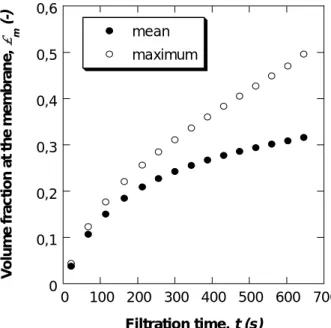
4.1 Evolution of the volume fraction versus filtration time
The simulation results (Figure 4) give the evolution of both the maximum ({) and mean value (z) of the volume fraction at the membrane surface. The increasing difference observed between these two values, which reaches more than 50% after 600 seconds, underlines an important heterogeneity of matter accumulation.
An illustration of this heterogeneity in mass accumulation is given in Figure 5, where the profile of the volume fraction as a function of the two dimensions of the hollow
fibre is given after 600 seconds for a mean permeate flux of 3.06×10⁻⁵ m.s-1. It should be noted that for the operating conditions corresponding to Figure 5, due to the pressure drop in the channel and to the development of the osmotic pressure at the membrane surface (according to equ. (10)), the local flux decreases along the membrane, ranging from 3.31×10⁻⁵ m.s-1 at the inlet to 2.78×10⁻⁵ m.s-1 at the end of the membrane.
This figure clearly shows that the matter accumulation is rather heterogeneous and is influenced by the hydrodynamics peculiar to the hollow fibre configuration, even if the Reynolds number (and therefore the wall shear stress) is relatively low (Re=147 at the channel entrance for this permeate flux). Even, if no experimental data are available in the literature in order to provide a strict comparison with these simulations in the inside/out configuration, the effect of hydrodynamic conditions is qualitatively corroborated by experiments of outside/in filtration [19].
To highlight the time dependence of matter accumulation, the axial volume fraction at the membrane surface is reported in Figure 6 for different filtration times ranging between 100 and 600 seconds, corresponding to filtered volumes of 3 to 18 L.m-2. Figure 6 shows that the volume fraction at the membrane reaches stationary values (for example before 300s at x = 0.6 m). Actually the accumulation behavior here appears to be a mix of two different behaviors:
• a zone, at the channel inlet, working as in cross-flow (with stationary
accumulation)
• a zone, at the end of the channel, working as in dead-end (with progressive accumulation).
It also shows that the proportion of the membrane working in dead-end mode (where mass accumulates) decreases with time. Two direct consequences can be drawn from this observation:
- the critical particle volume fraction (leading to the irreversible formation of a deposit) will be reached at the end of the hollow fibre;
- A comparison with “pure” dead-end filtration (the dotted line on Figure 6 after 600s of filtration) corresponding to an homogeneous accumulation which could take place at a flat sheet membrane, underlines that the critical condition will be reached faster when using a hollow fibre but only on a small part of the membrane.
4.2 Analysis of mass accumulation
A further analysis of the results can be made by considering the accumulated volume per unit membrane area (defined by equ. (11)), Vacc, corresponding to the total volume
of particle matter accumulated for a given axial position from the beginning of the filtration:
∫
⋅
=
wall r accr
V
0d
φ
(11)The evolution of the axial accumulated volume, Vacc, with the axial distance and for
different filtration times is shown in Figure 7. This figure illustrates that accumulation in the channel becomes more and more heterogeneous with increased filtration time. Whereas a flat sheet configuration would have resulted in a homogeneous matter accumulation, the hollow fibre configuration is influenced significantly by the slight tangential velocity: after 600 s of filtration, the last 600 mm of the membrane (50% of the porous part) contains 79% of the total accumulated mass.
Accumulation is higher at the end of the channel because of the thickening of the diffusive boundary layer (as in cross-flow conditions). Such a trend has already been experimentally proven by numerous studies in cross flow conditions and for different geometries. Simulations here show that this phenomena is accentuated in hollow fibre dead-end filtration because of the tangential velocity decrease in the axial direction (from 0.15 m.s-1 at the inlet to 0 m.s-1 at the end of the channel for dead-end filtration) resulting in a lower shear stress at the end of the channel, as is evident from the velocity profile shown in Figure 3.
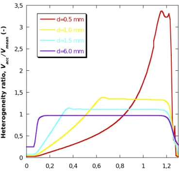
This heterogeneity can be quantified through the heterogeneity ratio, HR, defined as the ratio of the accumulated volume in the hollow fibre, V , over the mean accumulated acc volume, V , corresponding to homogeneous accumulation: the closer the value of this acc heterogeneity ratio is to 1, the more the matter accumulation is homogeneous. A HR value greater than one corresponds to the existence of a higher mass accumulation than would occur for a flat sheet membrane. This parameter has been used to quantify the effect of membrane diameter and filtration flux on the way accumulation occurs.
4.3 Effect of membrane configuration
Different diameter tubes were investigated in order to cover the range encountered in industrial applications: between 0.5 mm (dialysis fibres) up to 6mm (tubular membranes). The length of the tube was kept constant at 1.3m. All the results presented here correspond to a filtration flux of 110 L.h-1.m-2 leading to inlet velocities ranging
from 0.01 m.s-1 (for the 6 mm diameter tube) to 0.29 m.s-1 (for the 0.5 mm diameter tube) but having the same Reynolds number value at the inlet of the channel of 147.
The axial distribution of heterogeneity ratio after filtration of 9 L.m-2 (corresponding to 300 s) is presented in Figure 8. This figure underlines the statement that the heterogeneity decreases when the diameter increases; a 6 mm diameter membrane exhibits similar behaviour to a flat sheet membrane with a homogeneous accumulation over all the surface of the membrane. The time (i.e. filtered volume) dependence of this heterogeneity can be investigated by determining the percentage of membrane area working in dead-end filtration.
Simulations underline the fact that the membrane configuration is of great importance in the way matter accumulates at the surface. Such trends have already been theoretically and experimentally investigated for the outside/in hollow fibre configuration [18, 19]. Simulations here show that the use of an inside/out hollow-fibre membrane also introduces axial accumulation heterogeneities which can have important implications. However, if the accumulation is locally fastest in a hollow fibre than when using a flat sheet membrane, it is still located on a small percentage of the filtration surface, from which one can expect lower consequences on the overall process. Design of membranes, the effect of the position of the feed, constant pressure operation, etc. could be investigated using this CFD tool in order to find optimized conditions allowing the best control of fouling.
The effect of filtration flux is of interest as it is one of the parameters that can most easily be modified when running a filtration operation. One can observe from Figure 9 that the heterogeneity increases when the flux decreases. For example, at the end of the fibre, for a flux of 50 L.h-1.m-2, the accumulation is five times faster than what it would be for a flat sheet membrane. This can be explained by the important heterogeneity in the hydrodynamic conditions: the boundary layer thickness increases by a large amount due to the decreasing axial velocity along the channel. It has been shown by considering 1D modelling that the critical filtered volume is inversely proportional to the permeate flux: decreasing permeate flux allows longer filtration times before the formation of deposit starts [10]. The 2D modelling of a hollow fibre membrane shows that this conclusion should be moderated by the fact that reducing the flux also increases the heterogeneity in mass accumulation, which can lead to the appearance of a deposit at the end of the channel after a shorter time.
5. Conclusions
The description of the colloidal phase transition coupled with hydrodynamic and mass transfer equations allows a quantitative description of the filtration process through the evaluation of the dynamics of matter accumulation. Results highlight the heterogeneity of the mass accumulation and furthermore deposit formation at the membrane surface: for a constant flux of 110 L.h-1.m-2 and a 1 mm diameter hollow fibre, the accumulation can be, after 16 L m-2 of filtration, locally twice the value that would be reached homogeneously for a planar configuration. Conditions for deposit formation are then reached faster but the important information that the model provides is that this
accumulation occupies only a small part of the membrane. For a hollow fibre, the deposit formed on 15% of the membrane surface at the closed-end of the channel whereas it appears on the whole surface in the planar configuration. Simulation shows that this heterogeneity in mass accumulation rate and deposit coverage increases when the channel diameter is decreased or the permeate rate is decreased.
For hollow fibre and tubular configurations, simulations quantify the important interplay between the hydrodynamics, the dynamic establishment of concentration polarisation and the deposit formation during filtration of colloidal dispersions. Simulation results show that assumptions of homogeneous accumulation and instantaneous deposit formation which are classically used to model fouling are not appropriated in such configurations. Such simulations can be helpful not only to predict the formation of a deposit along the membrane channel but also to estimate the efficiency of relaxation or fouling removal. These simulations, developed using a commercial CFD code (ANSYS CFX), could then lead to an interesting tool to investigate the effect of process conditions (nature of the filtered colloids, membrane configuration, operating parameters ...) on its efficiency.
Acknowledgements
David Fletcher is grateful for funding from the CNRS to spend time at UMR 5503 in Toulouse developing this model.
References
[1] K.J. Howe, M.M. Clark, Fouling of microfiltration and ultrafiltration membranes by natural waters, Environmental Science & Technology 36 (2002) 3571-3576.
[2] P. Bacchin, M. Meireles, M., P. Aimar, Modelling of filtration: from the polarised layer to deposit formation and compaction, Desalination, 145 (2002) 139-146.
[3] B. Espinasse, Approche théorique et expérimentale de la filtration tangentielle de colloïdes : flux critique et colmatage, Thèse de l'Université Paul Sabatier, Toulouse, (2003).
[4] Y. Bessiere, Filtration frontale sur membrane : mise en évidence du volume filtré critique pour l'anticipation et le contrôle du colmatage, Thèse de l'Université Paul Sabatier, Toulouse, (2005).
[5] L.L. Zeman, A.L. Zydney, Microfiltration and ultrafiltration - Principles and applications, Marcel Dekker Inc., (1996).
[6] V. Chen, A.G. Fane, S. Madaeni, I.G. Wenten, Particle deposition during membrane filtration of colloids: transition between concentration polarization and cake formation, Journal of Membrane Science 125 (1997) 109-122.
[7] A.S. Jonsson, B. Jonsson, Ultrafiltration of colloidal dispersions--A theoretical model of the concentration polarization phenomena, Journal of Colloid and Interface Science, 180 (1996) 504-518.
[8] W.B. Russel, D.A. Saville and W.R. Schowalter, Colloidal dispersion, Cambridge University Press, 1989.
[9] B. Espinasse, P. Bacchin, P. Aimar, On an experimental method to measure critical flux in ultrafiltration, Desalination 146 (2002) 91-96.
[10] Y. Bessiere, N. Abidine, P. Bacchin, Low fouling conditions in dead-end filtration: evidence for a critical filtered volume and interpretation using critical osmotic pressure, Journal of Membrane Science 264 (2005) 37-47.
[11] J. Hermia, Constant pressure blocking filtration laws-application to power-law non-newtonian fluids, Trans. IChemE. 60 (1982) 183-187.
[12] P. Bacchin, B. Espinasse, Y. Bessiere, D.F. Fletcher, P. Aimar, Numerical simulation of colloidal dispersion filtration: description of critical flux and comparison with experimental results, Desalination 192 (2006) 74-81.
[13] R. Ghidossi, D. Veyret, P. Moulin, Computational fluid dynamics applied to membranes: State of the art and opportunities, Chem. Eng. Process., 45 (2006) 437-454. [14] R. Ghidossi, J.V. Daurelle, D. Veyret, P. Moulin, Simplified CFD approach of a hollow fiber ultrafiltration system, Chem. Eng. J. 123 (206) 117-125.
[15] D.E. Wiley, D.F. Fletcher, Techniques for computational fluid dynamics modelling of flow in membrane channels, J. Membr. Sci. 211 (2003) 127-137.
[16] D.F. Fletcher and D.E. Wiley, A computational fluid dynamics study of buoyancy effects in reverse osmosis, J. Membr. Sci. 245 (2004) 175-181.
[17] J.C. Chen, Q. Li, M. Elimelech, In situ monitoring techniques for concentration polarization and fouling phenomena in membrane filtration, Advances in Colloid and Interface Science 107 (2004) 83-108.
[18] T. Carroll and N.A. Booker, Axial features in the fouling of hollow-fibre membranes, J. Membr. Sci. 168 (2000) 203-212.
[19] G.S. Chang, A.G. Fane and T.D. Waite, Analysis of constant permeate flow filtration using dead-end hollow fiber membranes, J. Membr. Sci. 268 (2006) 132-141.
Figures captions
Figure 1. Evolution of a) osmotic pressure and b) diffusion coefficient with latex volume fraction. The symbols represent the experimental data (green symbols for latex in dispersed phase, red symbol for latex in condensed phase). The line represents the model fit.
Figure 2. Geometry definition for hollow fibre dead-end filtration
Figure 3: The fluid velocity along the channel for dead-end filtration at 110 Lh-1m-2. The black lines represent streamlines. Note that as the flow progresses from left to right the velocity falls due to extraction at the membrane surface.
Figure 4. Evolution of the colloid volume fraction at the membrane surface versus the filtration time (J=110 L.h-1.m-2)
Figure 5. Profile of the colloid volume fraction after 600s of filtration (J=110 L.h-1.m-2)
Figure 6. Time evolution of the colloid volume fraction at the membrane surface
Figure 7. Time evolution of the axial accumulated volume in the channel of the fibre
Figure 9. Heterogeneity ratio after filtration of 16 L.m-2 (d = 1 mm) for various mass fluxes
Figure 1 0 1 10-9 2 10-9 3 10-9 4 10-9 5 10-9 0 0,1 0,2 0,3 0,4 0,5 0,6 0,7 Dif fus io n c o e ffi cie n t ( m 2 .s -1 ) Volume fraction, φ (-) 0 5 103 1 104 1,5 104 2 104 2,5 104 0 0,1 0,2 0,3 0,4 0,5 0,6 0,7 Π reversible Π irreversible Os m o ti c p res s u re , Π (P a ) Volume fraction, φ (-) a) b)
Figure 2
r x
J(x)
Figure 3
z
Figure 4 0 0,1 0,2 0,3 0,4 0,5 0,6 0 100 200 300 400 500 600 700 mean maximum Vo lu m e f ra c tio n a t th e m e m b ra n e , φ m (-) Filtration time, t (s)
Figure 5 0 1 2 3 4 5 x 10 -5 0 0.5 1 0 0.1 0.2 0.3 0.4 0.5
y, distance from the wall (m) x, distance from the inlet (m)
v o lu m e f ra c ti on (-)
Figure 6 . 0 0,1 0,2 0,3 0,4 0,5 0,6 0,7 0 0,2 0,4 0,6 0,8 1 1,2 100 s 200 s 300 s 400 s 500 s 600 s V o lu m e f rac ti on a t th e m e m b ra n e , φm (-)
Figure 7 0 1 10-6 2 10-6 3 10-6 4 10-6 5 10-6 6 10-6 7 10-6 0 0,2 0,4 0,6 0,8 1 1,2 100 s 200 s 300 s 400 s 500 s 600 s A cc u mu la te d v o lu me, Va cc y (m 3 /m 2 )
Distance from the inlet, x (m)
« pure » dead-end
Vacc
Figure 8 0 0,5 1 1,5 2 2,5 3 3,5 0 0,2 0,4 0,6 0,8 1 1,2 d=0.5 mm d=1.0 mm d=1.5 mm d=6.0 mm H e te ro g e n e it y r a tio , V acc /V me a n (-)
Figure 9 0 1 2 3 4 5 6 0 0,2 0,4 0,6 0,8 1 1,2 J = 50 L.h-1.m-2 J = 80 L.h-1.m-2 J = 110 L.h-1.m-2 J = 140 L.h-1.m-2 H e tero g en e ity ra ti o , Vac c /Vme an (-)