HAL Id: hal-02380657
https://hal.archives-ouvertes.fr/hal-02380657
Submitted on 8 Dec 2020
HAL is a multi-disciplinary open access
archive for the deposit and dissemination of
sci-entific research documents, whether they are
pub-lished or not. The documents may come from
teaching and research institutions in France or
abroad, or from public or private research centers.
L’archive ouverte pluridisciplinaire HAL, est
destinée au dépôt et à la diffusion de documents
scientifiques de niveau recherche, publiés ou non,
émanant des établissements d’enseignement et de
recherche français ou étrangers, des laboratoires
publics ou privés.
To cite this version:
Nathalie Aubrun, Mathieu Sablik, Julien Esnay. Domino Problem Under Horizontal Constraints.
STACS 2020 37th International Symposium on Theoretical Aspects of Computer Science, 2020,
Mont-pellier, France. �10.4230/LIPIcs.STACS.2020.26�. �hal-02380657�
Nathalie Aubrun
Univ Lyon, CNRS, ENS de Lyon, Université Claude Bernard Lyon 1, LIP, F-69342, LYON Cedex 07, France
https://perso.ens-lyon.fr/nathalie.aubrun/ [email protected]
Julien Esnay
Institut de Mathématiques de Toulouse, Université Paul Sabatier, 118 route de Narbonne, F-31062 Toulouse Cedex 9, France
Univ Lyon, CNRS, ENS de Lyon, Université Claude Bernard Lyon 1, LIP, F-69342, Lyon Cedex 07, France
Mathieu Sablik
Institut de Mathématiques de Toulouse, Université Paul Sabatier, 118 route de Narbonne, F-31062 Toulouse Cedex 9, France http://www.math.univ-toulouse.fr/~msablik/index.html [email protected]
Abstract
The Domino Problem on Z2asks if it is possible to tile the plane with a given set of Wang tiles; it is a classical decision problem which is known to be undecidable. The purpose of this article is to parameterize this problem to explore the frontier between decidability and undecidability. To do so we fix some horizontal constraints H on the tiles and consider a new Domino Problem DPH: given
a vertical constraint, is it possible to tile the plane? We characterize the nearest-neighbor horizontal constraints where DPH is decidable using graphs combinatorics.
2012 ACM Subject Classification Theory of computation → Models of computation; Mathematics of computing → Combinatoric problems
Keywords and phrases Dynamical Systems, Symbolic Dynamics, Subshifts, Wang tiles, Undecidab-ility, Domino Problem, Combinatorics, Tilings, Subshifts of Finite Type
Digital Object Identifier 10.4230/LIPIcs.STACS.2020.26
Funding Nathalie Aubrun: Supported by the ANR project CoCoGro (ANR-16-CE40-0005). Julien Esnay: Supported by the ANR project CoCoGro (ANR-16-CE40-0005) and the Labex CIMI (project “Computational Complexity of Dynamical Systems”).
Mathieu Sablik: Supported by the Labex CIMI (project “Computational Complexity of Dynamical Systems”).
1
Introduction
The Domino Problem is a classical decision problem introduced by Wang [20] to study satisfaction procedures for some fragments of first-order logic. Considering a finite set of tiles that are squares with colored edges, called Wang tiles, we ask if it is possible to tile the plane with shifted copies of these tiles so that contiguous edges have the same color.
This question is also central in symbolic dynamics. A Zd-subshift of finite type is a set of
colorings of Zd by a finite alphabet, called configurations, and a finite set of patterns that
are forbidden to appear in those configurations. The set of tilings obtained when we tile the
plane with a Wang tile set is an example of Z2-subshift of finite type. In this setting, the
Domino Problem becomes: given a finite set of forbidden patterns, is the associated subshift of finite type empty?
On Z-subshifts of finite type, the Domino Problem is easily shown to be decidable. On
those over Z2, Wang conjectured the Domino Problem was decidable too, and produced
an algorithm of decision relying on the hypothetical fact that all subshifts of finite type contained some periodic configuration. However, his claim was disproved by Berger [5] who
proved that the Domino Problem over any Zd, d ≥ 2 is algorithmically undecidable. The
key of the proof is the existence of a Zd-subshift of finite type containing only aperiodic
configurations, on which computations are implemented. In the decades that followed, many alternative proofs of this fact were provided [19, 17, 14].
The exact conditions to cross this frontier between decidability and undecidability have been intensively studied under different points of view during the last decade. To explore
the difference of behavior between Z and Z2, the Domino Problem has been extended on
discrete groups [7, 11, 6, 1, 2] and fractal structures [4] in order to determine which types of structures can implement computation. The frontier is also studied by restraining complexity (number of patterns of a given size) [15] or bounding the difference between numbers of colors and tiles [13]. Additional dynamical constraints are also considered, such as block gluing property [18, Lemma 3.1] or minimality [9].
In this article we propose a new approach. We fix horizontal constraints H which define a
Z-subshift of finite type and consider the decision problem DPHthat given vertical contraints
V asks if it is possible to tile the plane. In other words, is the Z-subshift of finite type
defined by V compatible with the one defined by H? The purpose is to determine for which
horizontal constraints H the decision problem DPH is decidable.
This point of view has various motivations. First, one could eliminate horizontal con-straints that necessarily yield periodic configurations to perform a more efficient computer proof of the smallest aperiodic Wang tile set (reached with 11 Wang tiles in [12]). Second, a classical result is that every effective Z-subshift can be realized as an horizontal projection on
Z of a Z2-subshift of finite type [10, 3, 8]. However, in these constructions, the subshift in the
vertical direction is trivial. We can ask which other vertical subshift can be compatible with a given horizontal restriction: the result presented here is the first step to understand this. Finally, looking for the undecidable frontier under horizontal constraints helps us understand how to transfer information in order to implement computation.
Section 2 recalls the notions needed and formalizes the problem. Section 3 presents three categories of horizontal constraints that yield a decidable Domino Problem. Finally Section 4 proves that all others have an undecidable Domino Problem. This is shown by reduction: we prove that for any Wang tile set W , it is possible to add vertical constraints to these H so that the resulting subshift simulates W . These vertical constraints can control the horizontal transfer of information and implement any Wang tile set, and by extension computation. The proof faces combinatorial explosion into subcases and is based on a careful dichotomy.
2
Definitions
As a preliminary note, any interval mentioned in this article will be an interval of integers, unless explicitly stated otherwise.
2.1 Symbolic Dynamics
For a given finite set A called the alphabet, AZd is called the d-dimensional full shift over A.
Any x ∈ AZd, called a configuration, can be seen as a function from Zd to A and we write
x~v:= x(~v). For any ~k ∈ Zd define the shift map σ
~
k : AZd→ AZd such that σ~k(x)
~v= x~v+~k.
The product topology on AZd is generated by the metric d(x, y) = 2− inf{|~v||~v∈Zd,x
~
makes AZd a compact space. A pattern p is a finite configuration p ∈ APp where P p⊂ Zd
is finite. We say that a pattern p ∈ APp appears in a configuration x ∈ AZd – or that x
contains p – if there exists ~k ∈ Zd such that for every ~` ∈ Pp, σ ~ k(x)
~ `= p~`.
A Zd-subshift associated to a set of patterns F , called set of forbidden patterns, is defined
by XF= {x ∈ AZd | ∀p ∈ F , ∀~k ∈ Zd, ∃~` ∈ P p, σ ~ k (x)~`6= p~`}
that is, XF is the set of all configurations that do not contain any pattern from F . Note
that there can be several sets of forbidden patterns defining the same subshift X. A subshift can equivalently be defined as a closed set under both the topology and the shift map. If
X = XF with F finite, then X is called a Subshift of Finite Type, SFT for short.
For Z-subshifts, we will talk about nearest-neighbor SFTs if F ⊂ A{0,1}. For Z2-subshifts,
the most well-known nearest-neighbor SFTs are the Wang shifts, defined by a finite number of squared tiles with colored edges that must be placed matching colors called Wang tiles.
Formally, these tiles are quadruplets of symbols (te, tw, tn, ts). A Wang shift is described by
a finite Wang tile set, and local rules x(i, j)e= x(i + 1, j)wand x(i, j)n= x(i, j + 1)sfor all
integers i, j.
Note that Wang shifts are enough to encode any Z2-SFT, albeit changing the underlying
local rules and alphabet, so that a Z2-SFT is empty if and only if the corresponding Wang
shift is.
2.2 One-dimensional SFTs as graphs
As explained in [16], a nearest-neighbor SFT X = XF ⊂ AZ, with F ⊂ A2, can be described
as an oriented graph G = (V, ~E) with V = A and (a, b) ∈ ~E ⇔ ab /∈ F . This graph, that
encodes the allowed patterns, depends on A and F , thus two different descriptions of the same SFT will yield different graphs.
However one graph can be canonically associated to a nearest neighbor SFT from any other description of said SFT. It is the only one obtained by iterated suppression of all vertices with no incoming edge or no outgoing edge, and so there only remain biinfinite paths in the graph, that correspond to proper tilings of the line. This graph, denoted by G(X), is called the Rauzy graph (of order 1) of X. Note that a Rauzy graph can be made of one or several strongly connected components, SCC for short. In case it has several SCCs it can also contain transient vertices, that are vertices with no path from themselves to themselves. I Example 1. The two subshifts that are X = X{10,20,21,11,30,31,32,33}⊂ {0, 1, 2, 3}Z and
Y = Y{10,20,21,11}⊂ {0, 1, 2}Zare the same SFT. They have the same Rauzy graph made of
two SCCs {0} and {2}, and one transient vertex 1 (vertex 3 has been deleted from G(X) else it would be of out-degree 0).
This technique that algorithmically associates a graph to an SFT will be of great use in Section 4, because it means that our proof can mostly focus on combinatorics over graphs to describe all nearest-neighbor one-dimensional SFTs.
2.3 The Domino Problem
Define DP (Zd
) = {< H >| H is a nonempty Zd-SFT} where < H > is the encoding of the
SFT H using a finite alphabet and a finite set of forbidden patterns. DP (Zd) is a language
decidable, i.e. recognizable by a Turing Machine. Said otherwise, is it possible to find a
Turing Machine that takes as input any finite set of patterns F ⊂ AZd of rules and answers
YES if XF contains at least one configuration, and NO if it is empty?
It is widely known that DP (Z) is decidable, because the problem can be reduced to the emptiness of nearest-neighbor Z-SFTs, and finding a valid configuration in a nearest-neighbor SFT is equivalent, via what precedes, to finding a biinfinite path – hence a cycle – in a
finite oriented graph. On the contrary, DP (Z2) is undecidable [5, 19, 17, 14], and so is any
DP (Zd
) for d ≥ 2 by reduction to the undecidability of DP (Z2).
2.4 Framework
IDefinition 2. Let H, V ⊂ AZ be subshifts. The two-dimensional subshift
XH,V := {x ∈ AZ
2
| ∀i, j ∈ Z, (xk,j)k∈Z∈ H and (xi,`)`∈Z∈ V }
is called the combined subshift of H and V , and uses H as horizontal rules and V as vertical rules.
IRemark. The projection of the horizontal configurations that appear in XH,V does not
necessarily recover all of H; we may simply have a subset of it. Indeed, all configurations in
H will not necessarily appear because some of them may not be legally extended vertically.
An easy instance of this is choosing A = {0, 1}, H nearest-neighbor and forbidding 00 and
11, and V non-nearest-neighbor and forcing to alternate a 0 and two 1s: the resulting XH,V
is empty, although neither H nor V are. In some sense, said H and V are incompatible. The previous remark motivates the main problem we will study in the rest of this article: understanding when two one-dimensional SFTs are compatible to build a two-dimensional SFT, and by extension where the frontier between decidability and undecidability lies. This question is notably reflected by the following adapted version of the Domino Problem: IDefinition 3. Let H ⊂ AZ be an SFT. The Domino Problem depending on H is the language
DPH := {< V >| V ⊂ AZ is an SFT and XH,V 6= ∅}.
IRemark. It is important to understand that this Domino Problem is defined for a given H,
and its decidability depends on such a H we choose beforehand. Subshifts can be conjugate, this being defined as a continuous bijection that commutes with the shift maps. Although it allows to identify structurally identical subshifts from a dynamical point of view, these
subshifts remain different in how they can encode information. Indeed, some SFT H1and
H2 may be conjugate with DPH1 decidable but DPH2 undecidable. Consider for instance
the following Rauzy graphs and applications on finite words (extensible to biinfinite words):
a b β α γ φ : aa 7→ γ ab 7→ β ba 7→ α bb 7→ β ψ : α 7→ a β 7→ b γ 7→ a
These graphs describe conjugate SFTs through these applications, with φ(x)i+1 =
φ(xixi+1). However, as we will see in Section 3, the first graph has decidable DPH and the
3
Main result: frontier between decidability and undecidability
To understand where our future decidability conditions stem from, we study three examples: IExample 4. Consider the following Rauzy graphs:
G(H1) G(H2) G(H3)
Let us consider a “vertical” Z-SFT V . As long as one can build a single column respecting
the rules of V , this column can legally be juxtaposed with itself in XH1,V since any element of
H1 can be horizontally juxtaposed with itself due to the self-loop at each vertex. Conversely,
if XH1,V contains a configuration, then in particular it contains a single column respecting
the rules of V . Hence checking if XH1,V is empty is tantamount to checking if V is empty.
Since DP (Z) is decidable, DPH1 is easily decidable in this case.
The same reasoning can be applied to the two other cases: for H2 any pair of columns,
and for H3 any triplet of columns, can be juxtaposed with itself. This finite number of
columns makes the decidability of our Domino Problem at stake depend on the decidability of DP (Z). The extensive proof of this fact is located below Theorem 6.
With these three examples, we briefly saw how these three kinds of graphs yielded a
decidable DPH. The rest of this article will produce a proper proof of this and, more
importantly, will show that these three rather natural categories are in fact the only ones where decidability appears.
IDefinition 5. We say that an oriented graph G = (V, ~E) verifies condition D (for “Decid-able”) if all its SCCs have a type in common among the following list. A SCC S can be of none, one or several of these types:
for all vertices v ∈ S, we have (v, v) ∈ ~E) (we say that S is of reflexive type);
for all vertices v 6= w ∈ S such that (v, w) ∈ ~E, we have (w, v) ∈ ~E (we say that S is of
symmetric type; note that S = {v} a single vertex with a loop is also symmetric);
S =F Vi such that ∀v ∈ Vi, [(v, w) ∈ ~E ⇔ w ∈ Vi+1] with i meant modulo the number of
classes (we say that S is of state-split cycle type in reference to a term used in [16]; note that a partition with one unique class V0 causes S to be a single vertex with self-loop). ITheorem 6. Let H be a nearest-neighbor Z-SFT.
DPH is decidable ⇔ G(H) verifies condition D.
Proof. Proof of ⇐: assume G(H) verifies condition D. Then its SCCs share a common type, be it reflexive, symmetric, or state-split cycle. For each of these three cases, we produce an
algorithm that takes as input a Z-SFT V ⊂ AZ, and that returns YES if XH,V is nonempty,
and NO otherwise.
Let M be the maximal size of forbidden patterns in FV (since V is an SFT, such an
integer exists).
If G(H) has state-split cycle type SCCs: let L be the LCM of the number of Vis in each
component. If there is no rectangle of size L × M (|A|LM+ 1) (width × height) respecting
local rules of XH,V and containing no transient element, then answer NO. Indeed, any
transient elements. If there is such a rectangle R, then by the pigeonhole principle it
contains at least twice the same rectangle R0 of size L × M . To simplify the writing, we
assume that the rectangle that repeats is the one of coordinates [1, L] × [1, M ] inside
R where [1, L] and [1, M ] are intervals of integers, and that it can be found again with
coordinates [1, L] × [k, k + M − 1]. Else, we simply truncate a part of R so that it becomes true.
Define P := R|[1,L]×[1,k+M −1]. Since V has forbidden patterns of size at most M , and since
R respects our local rules and begins and ends with R0, P can be vertically juxtaposed
with itself (overlapping on R0).
P can also be horizontally juxtaposed with itself (without overlap). Indeed, one line of P uses only elements of one SCC of H (since elements of two different SCCs cannot be
juxtaposed horizontally, and we banned transient elements). Since L is a multiple of the length of all cycle classes, the first element in a given line can follow the last element in the same line. Hence all lines of P can be juxtaposed with themselves.
As a conclusion, P is a valid patch that can tile Z2 periodically. Therefore, XH,V is
nonempty; return YES.
If G(H) has symmetric type SCCs the construction is similar, but this time build a
rectangle R of size 2 × M (|A|2M + 1). Either we cannot find one and return NO; or we
can find one and from it extract a patch that tiles the plane periodically and return YES. Finally, if G(H) has reflexive type SCCs, the construction is even simpler than before.
Build a rectangle R of size 1 × M (|A|M+ 1); the rest of the reasoning is identical.
Proof of ⇒ is postponed to Section 4, and is done by contraposition. If G(H) does not verify
condition D, then for any Wang shift W we can algorithmically build some Z-SFT VW such
that XH,VW reproduces all configurations in W . If we were able to solve DPH, then there
would exist a Turing Machine M able to tell us if XH,V is empty for any Z-SFT V . But
then we could build a Turing Machine N taking as input any Wang shift W , building the
corresponding VW after the following construction, and by running M, N would be able to
tell us if XH,VW is empty or not. Then it could answer if W is empty or not; but determining
the emptiness or nonemptiness of every Wang shift is equivalent to DP (Z2) being decidable,
which is false. Hence, since DP (Z2) is undecidable, DPH is too. J
4
Encoding a Wang shift under horizontal constraints
We begin this section by presenting the core idea of our algorithmic construction to prove the direct implication by contraposition. Then, we introduce the vertical patterns needed to achieve it in a generic case, said generic case being based on a set of conditions C. Finally, we show that most graphs that do not verify condition D do verify condition C, and those which don’t only need a slight adaptation of our generic construction.
4.1 Core idea
We have a one-dimensional nearest-neighbor SFT H ⊂ AZ(“horizontal”) that does not verify
condition D, and we fix a Wang shift W with a set of N tiles τ = {τ1, ..., τN}.
The idea is to introduce a well-chosen one-dimensional SFT V ⊂ AZ(“vertical”) depending
on W so that XH,V encodes the full shift on N elements. Then, we refine V by adding
conditions on forbidden patterns, thus encoding exactly the configurations in W . Such a construction is done with the use of two main parts, that we will obtain by some carefully chosen forbidden patterns in V .
sync T0,0 sync T1,0 sync T2,0 sync T3,0 sync T4,0 sync T0,1 sync T1,1 sync T2,1 sync T3,1 sync T4,1 sync T0,2 sync T1,2 sync T2,2 sync T3,2 sync T4,2
(a) Basic depiction of sync parts
and coding parts that represent tiles of W (not to scale; actually unrealizable). sync T0,0 sync T1,0 sync T2,0 sync T3,0 sync T4,0 sync T0,1 sync T1,1 sync T2,1 sync T3,1 sync T4,1 sync T0,2 sync T1,2 sync T2,2 sync T3,2 sync T4,2
(b) Same construction adding
“buffers” between codings of tiles to be realizable. sync T0,0 T0,0 T0,0 T0,0 sync T1,0 T1,0 T1,0 T1,0 sync T2,0 T2,0 T2,0 T2,0 sync T3,0 T3,0 T3,0 T3,0 sync T4,0 T4,0 T4,0 T4,0 sync T0,1 T0,1 T0,1 T0,1 sync T1,1 T1,1 T1,1 T1,1 sync T2,1 T2,1 T2,1 T2,1 sync T3,1 T3,1 T3,1 T3,1 sync T4,1 T4,1 T4,1 T4,1 sync T0,2 T0,2 T0,2 T0,2 sync T1,2 T1,2 T1,2 T1,2 sync T2,2 T2,2 T2,2 T2,2 sync T3,2 T3,2 T3,2 T3,2 sync T4,2 T4,2 T4,2 T4,2 (c) Improved construction: we
encode vertically the horizontal restrictions between tiles of W . A tile of W (here T2,1) is
repres-ented in bold.
Figure 1 Steps of the core idea to reach the generic construction. Not to scale: the sync part
will be much bigger than the code part.
First, there are parts of synchronization, also called sync parts, that give some rigidity to our tilings. They precise where the actual coding parts can be, which letters of the alphabet can be used and where in these coding parts, and they ensure that you cannot glue patches together in an unexpected way. They are the frame of our construction. Second comes the filling: the coding parts. A given coding part simply codes a number between 1 and N , possibly several times.
In Figure 1a (our first rough attempt to encode a full shift on an alphabet of size N ), we suppose that our sync parts properly maintain this global structure. We notice that it offers an interesting opportunity to transmit information vertically. Since our coding parts are exactly aligned, once we have encoded the full shift over an alphabet of size N , it will suffice to add vertical conditions to our V to precise whether a coding part can be above another one.
However, horizontally Figure 1a overlooks two problems:
Since we must respect the horizontal conditions given by H, we cannot put any coding part next to any other one if we do not put some kind of buffer between the two; Even with this, we have no control on the horizontal transfer of information. The idea is to transmit this horizontal information vertically, since we can add vertical constraints. We can fix the first problem by setting a buffer (see Figure 1b) between two coding parts, a portion of column that contains no coding and which can be next to any coding part. Of course, we must ensure that this buffer cannot be anywhere in a configuration but obediently remains between two coding parts. The sync parts will be designed to handle this.
However, this does not solve our need for horizontal transmission of information. Hence a new idea: altering our coding parts so that they transmit information diagonally. We put several consecutive lines of them, shifted little by little, as illustrated in Figure 1c. That way, we can encode horizontal forbidden patterns vertically, because we can see vertically which coding part is on the right of the one we are considering. For instance, by looking vertically
we can know that the encoding of T1,1 is next to T2,1 and above T1,0, and thus restrict the
content of these codings.
In what follows, we will build Figure 1c in details, although some technicalities will be needed to preserve the integrity of our sync parts and to ensure that the coding of a tile of
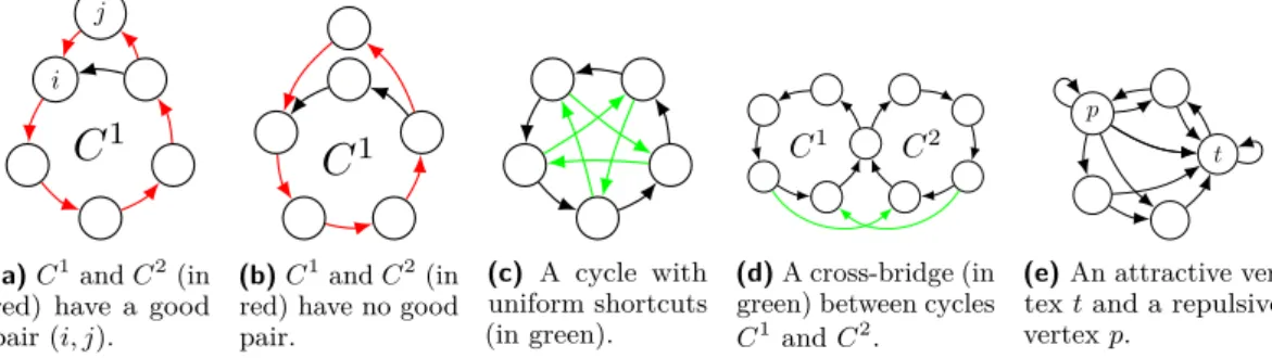
i j
C
1(a) C1and C2(in
red) have a good pair (i, j).
C
1(b) C1and C2(in
red) have no good pair. (c) A cycle with uniform shortcuts (in green). C2 C1 (d) A cross-bridge (in
green) between cycles C1and C2.
t p
(e) An attractive
ver-tex t and a repulsive vertex p.
Figure 2 Cases of compliance or not with elements of Condition C.
of W . Then, it can easily be refined by adding vertical rules so that the local rules of W are
ensured. Consequently, our newly built XH,V will properly simulate all configurations of W ,
allowing us to perform the rest of the proof of Theorem 6.
4.2 Generic construction
In this section, we describe a set of conditions on a nearest-neighbor SFT H that allows to build formally what we described informally in Section 4.1. In all that follows, we denote
elements of cycles with an index that is written modulo the length of the corresponding cycle.
The following definitions are illustrated in Figure 2.
IDefinition 7. Let C1 and C2 be two cycles in an oriented graph G, with elements denoted respectively c1
i and c2j. Let M := lcm(|C1|, |C2|).
We say that the cycles C1 and C2 contain a good pair if there is a pair (i, j) and
an integer 1 < l < M − 1 such that c1
i 6= c2j, c1i+1 6= c2j+1, . . . , c1i+l 6= c2j+l and c1i+(l+1) =
c2 j+(l+1), . . . , c 1 i+(M −1)= c 2 j+(M −1).
IDefinition 8. Let H ⊂ AZ be a one-dimensional nearest-neighbor SFT. We say that H
verifies condition C if G(H) = (V, ~E) contains two cycles C1 and C2, of elements denoted
respectively c1
i and c2j, with the following properties:
(i) |C1| ≥ 3;
(ii) C1 and C2 contain a good pair;
(iii) (there is no uniform shortcut neither in C1 nor in C2) There does not exist any k ∈ {0, 2, ..., |C1| − 1} such that for any c1
i ∈ C1, (c1i, c1i+k) ∈ ~E; and there does not
exist any k ∈ {0, 2, ..., |C2| − 1} such that for any c2
j ∈ C2, (c2j, c2j+k) ∈ ~E;
(iv) (there is no cross-bridge between C1 and C2) There are no i ∈ {0, ..., |C1| − 1} and
j ∈ {0, ..., |C2| − 1} with c1
i 6= c2j and c1i+1 6= cj+12 such that (c1i, c2j+1) ∈ ~E and
(c2
j, c1i+1) ∈ ~E;
(v) (there cannot be both an attractive vertex and a repulsive vertex for C1) Either there is no r ∈ C1∪ C2 such that for all c ∈ C1, (c, r) ∈ ~E, or there is no r ∈ C1∪ C2 such that for all c ∈ C1, (r, c) ∈ ~E.
IProposition 9. If G(H) verifies condition C, then DPH is undecidable.
The rest of the subsection is devoted to proving this result.
Let H with G(H) verifying condition C. We focus on encoding a full shift on an alphabet
τ of cardinality N . Then, the possibility to add vertical rules will allow us to encode any
Wang shift W using this alphabet, that is, to simulate the configurations of W as described in Section 4.1.
For the rest of the construction, we will name M := lcm(|C1|, |C2|) and K := 2|C1| +
|C2| + 3. We suppose that N ≥ 2 and do not focus on the trivial instance of W being a
monotile Wang shift.
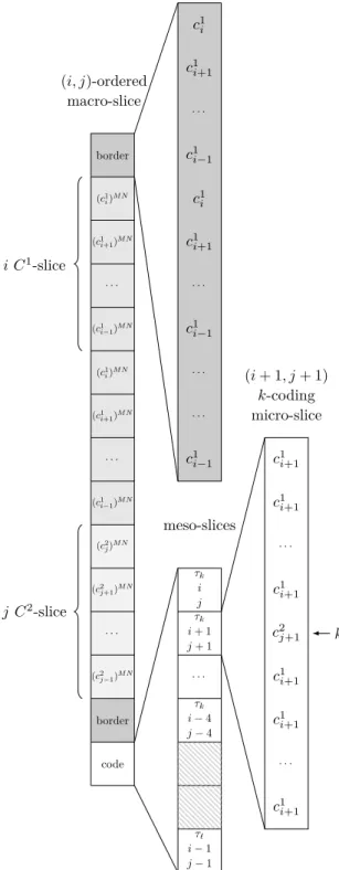
We refer to Figure 3a in all that follows. We use the term slice as a truncation of a column: it is a part of width 1 and of finite height. We use the following more specific denominations for the various scales of our construction:
A macro-slice is of height KM N . Any column is merely made of a succession of some specific macro-slices called ordered macro-slices (see below).
A meso-slice is of height M N . An ordered macro-slice is made of various meso-slices that ensure it carries information and is correctly aligned with neighboring ordered macro-slices (of neighboring columns).
A micro-slice is of height N . This subdivision is used inside code meso-slices (see below). Although any scale of slice could denote any truncation of column of the right size, we will only focus on specific slices that are meaningful because of what they contain, so that we can assemble them precisely. They are:
An (i, j) k-coding micro-slice is a micro-slice composed of N − 1 symbols c1
i and one
symbol c2j at position k. It encodes the kth tile of alphabet τ , unless c1i = c2j: it is then
called a buffer and encodes nothing.
An (i0, j0)-code meso-slice is made of M successive coding micro-slices starting with a
(i0, j0) coding micro-slice (that can encode anything). We add the vertical constraint that if c1
i 6= c2j, then the (i, j) k-coding micro-slice is vertically followed by the (i + 1, j + 1)
k-coding micro-slice. If c1i = c2j, the (i, j) k-coding micro-slice can be vertically followed by any (i + 1, j + 1) l-coding micro-slice. Note that there can be at most one such rupture
in the coding since C1 and C2 contain a good pair; k is then called the main-coded tile,
and l the side-coded tile.
An i-border meso-slice is made of |CM1|N times the vertical repetition of elements of the
cycle C1, starting at c1
i.
A c1i meso-slice is made of M N times the vertical repetition of element c1i, denoted
(c1
i)MN in Figure 3a. Same for a c2j meso-slice.
The succession of a c1
i meso-slice, then a c1i+1 meso-slice, ..., then a c1i−1meso-slice is called
a i C1-slice (of height M N |C1|). Similarly, we define a j C2-slice (of height M N |C2|).
Finally, a (i, j)-ordered macro-slice is the succession of a i-border meso-slice, a i C1-slice,
a second i C1-slice, a j C2-slice, a i-border meso-slice, and finally a (i, j)-code meso-slice.
Now, the patterns we authorize in V are exactly the cyclic permutations of (i0+ k, j0+
k)-ordered macro-slices with some good pair (i0, j0) and k ∈ {0, . . . , M − 1}. As a consequence,
a given column is simply the repetition of a given (i, j)-ordered macro-slice. We prove below
that it is enough for our resulting XH,V to simulate a full shift on τ .
We say that two legally adjacent columns are aligned if they are subdivided into ordered macro-slices exactly on the same lines. We say that two adjacent and aligned columns are
synchronized if any (i, j)-ordered macro-slice of the first one is followed by a (i + 1, j +
1)-ordered macro-slice in the second one.
IProposition 10. In this construction, two legally adjacent columns are aligned up to a vertical translation of size at most 2|C1| − 1 of one of the columns.
Proof. If two columns, call them K1 and K2, can be legally juxtaposed such that they
are not aligned even when vertically shifted by 2|C1| − 1 elements, it means that one of
the border meso-slices of K1 has at least 2|C1| vertically consecutive elements that are
26:10 Domino Problem Under Horizontal Constraints c1 i c1 i+1 . . . c1 i−1 c1 i c1 i+1 . . . c1i−1 . . . . . . c1 i−1 (i, j)-ordered macro-slice border (c1 i)M N (c1 i+1)M N . . . (c1 i−1)M N (c1 i)M N (c1 i+1)M N . . . (c1 i−1)M N (c2 j)M N (c2 j+1)M N . . . (c2 j−1)M N border code i C1-slice j C2-slice meso-slices τk i j τk i + 1 j + 1 . . . τk i − 4 j − 4 τ` i − 1 j − 1 (i + 1, j + 1) k-coding micro-slice c1 i+1 c1 i+1 . . . c1 i+1 c2 j+1 c1 i+1 c1 i+1 . . . c1 i+1 k
(a) Columns allowed, for (i, j) in the orbit of a good pair.
Here c1i−3= c2j−3and c1i−2= c2j−2, forming buffers in the code meso-tile. border (c1 i)M N (c1 i+1)M N ... (c1 i−1)M N (c1 i)M N (c1 i+1)M N ... (c1 i−1)M N (c2 j)M N (c2 j+1)M N ... (c2 j−1)M N border code border (c1 i)M N (c1 i+1)M N ... (c1 i−1)M N (c1 i)M N (c1 i+1)M N ... (c1 i−1)M N (c2 j)M N (c2 j+1)M N ... (c2 j−1)M N border code (c1 i+1)M N ... (c1 i−1) M N (c1 i)M N (c1 i+1)M N ... (c1 i−1) M N (c2 j) M N (c2 j+1)M N ... (c2 j−1) M N border code border (c1 i) M N (c1 i+1)M N ... (c1 i−1)M N (c1 i) M N (c1 i+1) M N ... (c1 i−1)M N (c2 j)M N (c2 j+1)M N ... (c2 j−1)M N border code
(b) Faulty alignment of adjacent
columns.
Since 2|C1| < M N , at least |C1| successive elements among the ones of the border meso-slice
are horizontally followed by elements that are part of the same meso-slice. If this is a code
meso-slice, simply consider the other border meso-slice of K1(the first you can find, above
or below, before repeating the pattern cyclically): this one must be in contact with a c1
i
or c2
j meso-slice instead. Either way, we obtain that a border meso-slice has at least |C1|
successive elements that are horizontally followed by some t meso-slice made of a single
element t. Hence if we suppose that juxtaposing K1 and K2 this way is legal, it means that
in H all the elements of C1 lead to t, i.e t is an attractive vertex. Either this is forbidden, or
the “reverse” reasoning where we focus on the borders of K2 proves that there is also an
element p used in a Cj slice of K
1 that leads to every element of C1; that is, a repulsive
vertex. We forbade any graph that had both, hence we reach a contradiction here. We obtain
the proposition we announced. J
IProposition 11. In this construction, two legally adjacent columns are always aligned and synchronized.
Proof. Proposition 10 states that two adjacent columns K1 and K2 are always, in some
sense, approximately aligned (up to a vertical translation of size at most 2|C1| − 1). If the
two columns are indeed slightly shifted, then any meso-slice of the C1 slice of K
1 (consisting
only of the repetition of some c1
i) is horizontally followed by two different meso-slices in K2.
Being different, at least one of them is not c1i+1 but some c1i+k, k ∈ {2, ..., |C1|}. This is true
with the same k for all values of i because all meso-slices representing c1
i are repeated twice
so that there is no “border effect”. We obtain something that contradicts our assumption that
C1 has no uniform shortcut. Hence there is no vertical shift at all between two consecutive
columns. Thus our construction ensures that two adjacent columns are always aligned.
It is easy to see that a meso-slice made only of c1
i in column K1 is horizontally followed,
because the columns are aligned, by a meso-slice made only of c1
i+k in column K2. This k is
once again independent of the i because inside a macro-slice, meso-slices respect the order of
cycle C1. But because C1has no uniform shortcut, we must have k = 1. The reasoning is
the same for the C2 slice, and we use the fact that C2 has no shortcut either. Hence our
columns are synchronized. J
With these properties, we have ensured that our structure is rigid: our ordered macro-slices are aligned just as we expected. The last fact to check is the transmission of information between horizontally aligned code meso-slices (since, by the structure of a code meso-slice, the vertical transmission is guaranteed).
We have to ensure that, every M horizontally aligned coding micro-slices, we have a succession of buffers (a (i, j)-coding micro-slice that does not encode information because
c1
i = c2j) then of non-buffers. Furthermore, we ask that all the buffers follow each other so
that we get some distinct “coding zone” and “buffer zone”. This is actually simply deduced from the fact that we only authorized as ordered macro-slices the ones based on the orbit of a good pair (see Definition 7).
Now, in which situation can there be a problem of horizontal transmission of the encoded tile between two micro-slices? Suppose we have a (i, j) micro-slice then a (i + 1, j + 1)
micro-slice. A problem of transmission would mean that c1
i can be followed by c2j+1, and c2j
by c1
i+1. A problem of transmission also assumes that we transmit something, hence we don’t
consider buffer micro-slices: necessarily c1
i 6= c2j and c1i+16= c2j+1. Then we would contradict
assumption (iv) “no cross-bridge” (which was assumed precisely to prevent this case). As a consequence of all this, every M micro-slices starting with a buffer micro-slice, horizontally successive coding micro-slices encode exactly one element of τ , since there is one single coding zone and the coded tile is correctly transmitted.
b
a
c
a a c b b c c c c c a a c b b c c c a c a b c b c c c a a c b b c c c c c a a c b b c c c a c a b c b c c c a a c b b c c c c c a a c b b c c c a c a b c b c c c a c a b c b c c cFigure 4 Some Rauzy graph and several associated code meso-slices for |τ| = 3. Here are
horizontally successively encoded τ3, τ1, τ2and τ2, the number being indicated by the location of the
line of c’s.
In the end, we proved that if we were able to find such C1 and C2 complying with
condition C, they would be enough to build the construction we desire: a full shift on N elements. Then, to encode only configurations that are valid in W , we forbid the following additional vertical patterns:
the code meso-slices that would contain both the main-coded kth tile and the side-coded
lth tile if tile k cannot be horizontally followed by tile l in W ;
and the vertical succession of two ordered macro-slices that would contain code meso-slices with two main-coded tiles that cannot be vertically successive in W .
With this, we proved Proposition 9.
4.3 Proof of Theorem 6 for one strongly connected component
We suppose that H ⊂ AZis a one-dimensional nearest-neighbor SFT such that its Rauzy
graph does not verify condition D and is made of only one SCC.
Note that G(H), since it does not verify condition D, contains at least one loopless vertex, and one unidirectional edge.
The idea is to divide the possible graphs into various cases. This way, one has a standard
procedure to find convenient C1and C2inside any graph to perform the generic construction.
Of course, for some specific cases, we won’t meet condition C even if H does not verify condition D. However, we will punctually adapt the generic construction to these specificities.
Table 1 Table of the main cases, each of them illustrated with an example (the C2
on which we perform the generic construction is in red).
Loops No loop
Bidirectional edges No bidirectional edge
v w C1 v w u C1 v a u C1 v w u C1 v w C1 C1 C1 C1
The division into cases is presented in a disjunctive fashion, see Table 1: Is there a loop on a vertex?
If YES: Is there a unidirectional edge (v, w) ∈ ~E so that v is loopless and w has a loop
(or the reverse, which is similar)?
If YES: This is Case 1.1. We can find C1 and C2 that check condition C with
the exception of the possible presence of both an attractive and a repulsive vertices. However, Proposition 10 is verified anyway because choosing the smallest possible cycle containing such v and w, v has in-degree 1, a property that allows for an easy synchronization.
If NO: Do unidirectional edges have loopless vertices?
∗ If YES: This is Case 1.2. We can find C1 and C2 that check condition C, possibly
by reducing to a situation encountered in case 2.2.
∗ If NO: This is Case 1.3. This one generates some exceptional graphs with 4 or 5
vertices that do not check condition C and must be treated separately. However, technical considerations prove that our generic construction still works.
If NO: Is there a bidirectional edge?
If YES: Is there a cycle of size at least 3 that contains a bidirectional edge?
∗ If YES: This is Case 2.1. We can find C1 and C2 that verify condition C rather
easily.
∗ If NO: This is Case 2.2, in which checking condition C is also easy.
If NO: Is there a minimal cycle with a path between two different elements of it, say
c1
0 and c1k, that does not belong to the cycle?
∗ If YES: Can we find such a path of length different from k?
· If YES: This is Case 3.1, a rather tedious case, but we can find cycles C1 and C2
that verify condition C nonetheless.
· If NO: This is Case 3.2, which relies heavily on the fact that G(H) is not of
state-split cycle type to find cycles that verify condition C.
∗ If NO: This is Case 3.3, an easy case to find cycles that verify condition C.
4.4 Proof of Theorem 6 for multiple strongly connected components
The idea if H has several SCCs is to build one, by products of SCCs, that is none of the three types that constitute condition D. We can then apply what we did in the previous subsections.
The direct product S1× S2 of two SCCs S1and S2 is made of pairs (s1, s2), where an
edge exists between two pairs if and only if edges exist in both S1 and S2 between the
corresponding vertices. It can be used in our construction by forcing pairs of elements (s1, s2) ∈ S1× S2to be vertically one on top of the other.
Since H does not verify condition D, it has a non-reflexive SCC S1, a non-symmetric
SCC S2 and a non-state-split SCC S3 (two of them being possibly the same). But then:
Since S1is non-reflexive, no SCC of S1× S2× S3 is reflexive. Indeed, since S1is strongly
connected, all vertices of S1are represented in any SCC C of that graph product, meaning
that for any s1∈ S1 there is at least one vertex of the form (s1, ∗, ∗) in C. But if C had
loop on all its vertices, then in particular S1 would be reflexive.
Similarly, since S2is non-symmetric, no SCC of S1× S2× S3 is symmetric.
Finally, since S3 is non-state-split, no SCC of S1× S2× S3 is a state-split cycle. Indeed,
suppose S is such a state-split SCC of the direct product. It can be written as a collection
new classes (Wi)i∈I, with some elements of S3that possibly appear in several of these.
Let c be any vertex in S3 that appears at least twice with the least difference of indices
between two classes where it appears; say c ∈ Wi and c ∈ Wi+k. Since S is state-split, all
elements in Wi+1 are exactly the elements of S3 to which c leads. But it is the same for
Wi+k+1. Hence Wi+1= Wi+k+1. From this we deduce that Wi= Wi+k for any i, using
the fact that indices are modulo |I|. Since k is the smallest possible distance between
classes having a common element, classes from (Wi)i∈{0,...,k−1} are all disjoint; and they
obviously contain all vertices from S3. Now simply consider these classes W0to Wk−1:
you get the proof that S3 is state-split.
Perspectives
Nearest-neighbor conditions are strong constraints, hence it is rather coherent that apart
from some very simple graphs the undecidability of DPH is systematic. Investigation has
begun about non-nearest-neighbor constraints, for which there seem to be more graphs with a decidable Domino Problem, this set of graphs possibly being non-recursive. For instance, the graph below is of decidable Domino Problem.
aa
ab ba
bb
Another perspective would be to generalize these results to Zd: we fix restrictions on a
Zk-SFT with k < d and look at the consequent decidability for Zd-SFTs. It is immediate
that if d − k ≥ 2 then we can reduce to DP (Z2) so this new problem is always undecidable.
However, the d − k = 1 case – that is, fixing a hyperplane – is still open.
References
1 Nathalie Aubrun, Sebastián Barbieri, and Emmanuel Jeandel. About the Domino Problem for Subshifts on Groups, chapter 9, pages 331–389. Springer International Publishing, 2019. doi:10.1007/978-3-319-69152-7_9.
2 Nathalie Aubrun, Sebastián Barbieri, and Etienne Moutot. The domino problem is undecidable on surface groups. In 44th International Symposium on Mathematical Foundations of Computer Science, MFCS 2019, August 26-30, 2019, Aachen, Germany, pages 46:1–46:14, 2019. doi: 10.4230/LIPIcs.MFCS.2019.46.
3 Nathalie Aubrun and Mathieu Sablik. Simulation of Effective Subshifts by Two-dimensional Subshifts of Finite Type. Acta Appl. Math., 126:35–63, 2013. doi:10.1007/ s10440-013-9808-5.
4 Sebastián Barbieri and Mathieu Sablik. The domino problem for self-similar structures. In Pursuit of the universal, volume 9709 of Lecture Notes in Comput. Sci., pages 205–214. Springer, [Cham], 2016. doi:10.1007/978-3-319-40189-8_21.
5 Robert Berger. Undecidability of the Domino Problem, volume 66 of Memoirs AMS. American Mathematical Society, 1966.
6 David B. Cohen. The large scale geometry of strongly aperiodic subshifts of finite type. ArXiv e-prints, December 2014. arXiv:1412.4572.
7 David B. Cohen and Chaim Goodman-Strauss. Strongly aperiodic subshifts on surface groups. ArXiv e-prints, October 2015. arXiv:1510.06439.
8 Bruno Durand, Andrei E. Romashchenko, and Alexander Shen. Fixed-point tile sets and their applications. J. Comput. Syst. Sci., 78(3):731–764, 2012. doi:10.1016/j.jcss.2011.11.001. 9 Silvère Gangloff and Mathieu Sablik. Simulation of minimal effective dynamical systems
on the cantor sets by minimal tridimensional subshifts of finite type. Prépublication (http://arxiv.org/abs/1806.07799), 2018.
10 Michael Hochman. On the dynamics and recursive properties of multidimensional sym-bolic systems. Inventiones mathematicae, 176(1):131, December 2008. doi:10.1007/ s00222-008-0161-7.
11 Emanuel Jeandel. Aperiodic subshifts of finite type on groups. https://hal.inria.fr/hal-01110211, 2015.
12 Emmanuel Jeandel and Michaël Rao. An aperiodic set of 11 wang tiles. CoRR, abs/1506.06492, 2015. arXiv:1506.06492.
13 Emmanuel Jeandel and Nicolas Rolin. Fixed parameter undecidability for wang tilesets. In Proceedings 18th international workshop on Cellular Automata and Discrete Complex Systems and 3rd international symposium Journées Automates Cellulaires, AUTOMATA & JAC 2012, La Marana, Corsica, September 19-21, 2012., pages 69–85, 2012. doi:10.4204/EPTCS.90.6.
14 Jarkko Kari. The tiling problem revisited (extended abstract). In Jérôme Durand-Lose and Maurice Margenstern, editors, Machines, Computations, and Universality, pages 72–79, Berlin, Heidelberg, 2007. Springer Berlin Heidelberg. doi:10.1007/978-3-540-74593-8_6.
15 Jarkko Kari and Etienne Moutot. Decidability and periodicity of low complexity tilings. CoRR, abs/1904.01267, 2019. arXiv:1904.01267.
16 Douglas Lind and Brian Marcus. Symbolic Dynamics and Coding. Cambridge University Press, 1995.
17 Shahar Mozes. Tilings, substitution systems and dynamical systems generated by them. Journal d’Analyse Mathématique, 53(1):139–186, December 1989. doi:10.1007/BF02793412.
18 Ronnie Pavlov and Michael Schraudner. Entropies realizable by block gluing Zd shifts of finite type. Journal d’Analyse Mathématique, 126(1):113–174, April 2015. doi:10.1007/ s11854-015-0014-4.
19 Raphael M. Robinson. Undecidability and nonperiodicity for tilings of the plane. Inventiones mathematicae, 12(3):177–209, September 1971. doi:10.1007/BF01418780.
20 Hao Wang. Proving theorems by pattern recognition – II. The Bell System Technical Journal, 40(1):1–41, 1961. doi:10.1002/j.1538-7305.1961.tb03975.x.