On polynomially integrable Birkhoff billiards on surfaces of constant curvature.

(1)

HAL Id: ensl-01664204

https://hal-ens-lyon.archives-ouvertes.fr/ensl-01664204v3

Submitted on 21 Nov 2019

HAL is a multi-disciplinary open access

archive for the deposit and dissemination of sci-entific research documents, whether they are pub-lished or not. The documents may come from teaching and research institutions in France or

L’archive ouverte pluridisciplinaire HAL, est destinée au dépôt et à la diffusion de documents scientifiques de niveau recherche, publiés ou non, émanant des établissements d’enseignement et de recherche français ou étrangers, des laboratoires

On polynomially integrable Birkhoff billiards on surfaces

of constant curvature.

Alexey Glutsyuk

To cite this version:

Alexey Glutsyuk. On polynomially integrable Birkhoff billiards on surfaces of constant curvature.. Journal of the European Mathematical Society, European Mathematical Society, In press. �ensl-01664204v3�

(2)

On polynomially integrable Birkhoff billiards on

surfaces of constant curvature

Alexey Glutsyuk∗†‡ February 20, 2019

Abstract

The polynomial version of Birkhoff Conjecture on integrable bil-liards on complete simply connected surfaces of constant curvature (plane, sphere, hyperbolic plane) was first stated, studied and solved in a particular case by Sergei Bolotin in 1990-1992. Here we present a complete solution of the polynomial version of Birkhoff Conjecture. Namely we show that every polynomially integrable real bounded pla-nar billiard with C2-smooth connected boundary is an ellipse. We ex-tend this result to billiards with piecewise-smooth and not necessar-ily convex boundary on arbitrary two-dimensional simply connected complete surface of constant curvature: plane, sphere, Lobachevsky– Poincar´e (hyperbolic) plane; each of them being modeled as a plane or a (pseudo-) sphere in R3 _{equipped with appropriate quadratic form.} Namely, we show that a billiard is polynomially integrable, if and only if its boundary is a union of confocal conical arcs and appropriate geodesic segments. We also present a complexification of these results. These are joint results of Mikhail Bialy, Andrey Mironov and the author. The proof is split into two parts. The first part is given in two papers by Bialy and Mironov (in Euclidean and non-Euclidean cases respec-tively). Their geometric construction reduced the Polynomial Birkhoff Conjecture to a purely algebro-geometric problem to show that an ir-reducible algebraic curve in CP2 with certain properties is a conic. They have shown that its singular and inflection points lie in the com-plex light conic of the above-mentioned quadratic form. In the present paper we solve the above algebro-geometric problem completely.

∗

CNRS, France (UMR 5669 (UMPA, ENS de Lyon) and UMI 2615 (Interdisciplinary Scientific Center J.-V.Poncelet)), Lyon, France. E-mail: aglutsyu@ens-lyon.fr

†

National Research University Higher School of Economics, Russian Federation ‡

Supported by part by RFBR grants 13-01-00969-a, 16-01-00748, 16-01-00766 and ANR grant ANR-13-JS01-0010.

(3)

1 Introduction

1.1 Main results

The famous Birkhoff Conjecture deals with strictly convex bounded planar billiards with smooth boundary. Recall that a caustic of a planar billiard Ω ⊂ R2 is a curve C such that each tangent line to C reflects from the boundary of the billiard to a line tangent to C. A billiard Ω is called Birkhoff caustic-integrable, if a neighborhood of its boundary in Ω is foliated by closed caustics, and the boundary ∂Ω is a leaf of this foliation. It is well-known that each elliptic billiard is integrable, see [40, section 4]. The Birkhoff Conjecture states the converse: the only Birkhoff caustic-integrable convex bounded planar billiard with smooth boundary is an ellipse.1

Let now Σ be a two-dimensional surface with a Riemannian metric, Ω ⊂ Σ be a connected domain2 with piecewise smooth boundary. The billiard flow Btacts on the tangent bundle T Σ|Ω as follows. A point (Q, P ) ∈ T Σ|Ω,

Q ∈ Ω, P ∈ TQΣ moves along a trajectory of the geodesic flow of the surface

Σ until Q hits the boundary ∂Ω. While hitting the boundary, the point Q remains unchanged, and the velocity vector P is reflected from the boundary to the vector P∗ according to the usual reflection law: the angle of incidence equals to the angle of reflection; |P | = |P∗|. Afterwards the new point (Q, P∗) again moves along a trajectory of the geodesic flow etc. The billiard flow thus defined, which can be viewed as a geodesic flow with impacts on T Σ|Ω, has an obvious first integral: the absolute value |P | of the velocity. A

strictly convex billiard Ω with smooth boundary is called integrable in the Liouville sense, if its flow has an additional first integral independent with

1

This conjecture, classically attributed to G.Birkhoff, was published in print only in the paper [37] by H. Poritsky, who worked with Birkhoff as a post-doctoral fellow in late 1920-ths.

(5)

|P | on the intersection with T Σ|_Ω of a neighborhood of the unit tangent bundle to the boundary.

The notions of a caustic and Birkhoff caustic-integrability extend to the case of a strictly convex domain Ω on an arbitrary surface Σ equipped with a Riemannian metric, with lines replaced by geodesics. The Liouville and Birkhoff caustic integrabilities are equivalent: it is a well-known folklore fact. There is an analogue of the Birkhoff Conjecture for billiards on a sim-ply connected complete Riemannian surface of non-zero constant curvature: sphere or hyperbolic (Lobachevsky–Poincar´e) plane. This is also an open problem.

The particular case of the Birkhoff Conjecture, when the additional first integral is supposed to be polynomial in the velocity components, motivated the next definition and conjecture.

Definition 1.1 Let Σ be a two-dimensional surface with Riemannian met-ric, and let Ω ⊂ Σ be a domain with piecewise smooth boundary. We say that the billiard in Ω is polynomially integrable, if its flow has a first integral on T Σ|Ω that is a polynomial in the velocity P and whose restriction to the

hypersurface {|P | = 1} is non-constant.

Definition 1.2 Let Σ be as above, and let Ω ⊂ Σ be a domain with piece-wise smooth boundary. We say that Ω is analytically integrable, if there exists a first integral analytic in P on a neighborhood in T Σ|Ω of the zero

section of the tangent bundle T Σ|Ω that is not a function of just the

mod-ulus |P |. In addition, it is required that there exists a r > 0 such that the integral is defined for all (Q, P ) with Q ∈ Ω and |P | ≤ r and its Taylor series in P converges uniformly in the above (Q, P ).

Note that all the integrals under question, which are defined over an open domain Ω, should be invariant under the geodesic flow in Ω and under the reflections from its boundary.

Remark 1.3 The following facts are well-known:

- Analytic integrability implies polynomial integrability, since each ho-mogeneous part in P of an analytic integral is a first integral itself, see [32, p. 107] (the converse is obvious);

- In the case, when Σ is a simply connected complete surface of constant curvature and the boundary ∂Ω is smooth and connected, polynomial inte-grability is equivalent to the existence of a polynomial integral as above in a neighborhood of the unit tangent bundle to ∂Ω in T Σ|Ω, by S.V.Bolotin’s

(6)

that is just polynomial in P is globally analytic on T Σ, see [17, proof of proposition 2] and Theorem 1.22.

The Polynomial Birkhoff Conjecture states that if a convex planar billiard with smooth boundary is polynomially integrable, then its boundary is a conic. The Polynomial Birkhoff Conjecture together with its gener-alization to billiards with piecewise smooth (may be non-convex) bound-aries on simply connected complete surfaces of constant curvature was first stated and studied by S.V.Bolotin [16, 17] and later studied in joint papers of M.Bialy and A.E.Mironov [10, 11, 12]. In the present paper we give a complete solution of the Polynomial Birkhoff Conjecture in full generality (Theorems 1.6 and 1.21).

Remark 1.4 The Polynomial Birkhoff Conjecture and its generalization are important and interesting themselves, independently on a potential solu-tion of the classical Birkhoff Conjecture. They lie on the crossing of different domains of mathematics, first of all, dynamical systems, algebraic geometry and singularity theory. They are not implied by the classical Birkhoff Con-jecture. For the general case of piecewise-smooth boundaries this is obvious. Even in the case of smooth convex boundary, while the polynomiality con-dition is a very strong restriction, the concon-dition of just non-constance of a polynomial integral on the unit velocity level hypersurface is topologically weaker than the independence condition in the Liouville integrability, which requires independence of the additional integral and the energy on a whole neighborhood in T R2|_Ω of the unit tangent bundle to the boundary.

Without loss of generality we consider simply connected complete sur-faces Σ of constant curvature equal to 0 or ±1: one can make non-zero constant curvature equal to ±1 by multiplication of metric by constant fac-tor; this changes neither geodesics, nor polynomial integrability. Thus, Σ is either the Euclidean plane, or the unit sphere, or the Lobachevsky–Poincar´e hyperbolic plane. It is modeled as one of the three following surfaces in the space R3 _{with coordinates x = (x}

1, x2, x3) equipped with the quadratic form

< Ax, x >, A ∈ {diag(1, 1, 0), diag(1, 1, ±1)}, < x, x >= x2₁+ x2₂+ x2₃. - Euclidean plane: Σ = {x3 = 1}, A = diag(1, 1, 0).

- The unit sphere: Σ = {x2₁+ x2₂+ x2₃= 1}, A = Id. - The hyperbolic plane: Σ = {x2

1 + x22 − x23 = −1} ∩ {x3 > 0}, A =

diag(1, 1, −1).

The metric of constant curvature on the surface Σ under question is induced by the quadratic form < Ax, x >. The geodesics on Σ are its

(7)

intersections with two-dimensional vector subspaces in R3. The conics on Σ are its intersections with quadrics {< Cx, x >= 0} ⊂ R3, where C is a real symmetric 3 × 3-matrix.

Example 1.5 The billiard in a disk in R2(x1,x2) centered at 0 has first

inte-gral x1P2− P1x2 linear in P . The billiard in any conic in any of the above

surfaces Σ has an integral quadratic in P , see [17, proposition 1].

Theorem 1.6 Let a billiard in Σ with a C2-smooth connected boundary be polynomially integrable. Let its boundary be not contained in a geodesic. Then the billiard boundary is a conic (or a connected component of a conic). Corollary 1.7 Every bounded polynomially integrable planar billiard with a C2-smooth connected boundary is an ellipse.

Below we extend the above theorem to billiards with countably piecewise smooth boundaries, see the following definition.

Definition 1.8 A domain Ω ⊂ Σ has countably piecewise (Cr-) smooth boundary, if ∂Ω consists of the two following parts:

- the regular part: an open and dense subset ∂Ωreg ⊂ ∂Ω, where each

point X ∈ ∂Ωreg has a neighborhood U = U (X) ⊂ Σ such that the

inter-section U ∩ ∂Ω is a (Cr-) smooth one-dimensional submanifold in U ; - the singular part: the closed subset ∂Ωsing = ∂Ω \ ∂Ωreg⊂ ∂Ω.

Remark 1.9 In the above definition the regular part of the boundary is always a dense and at most countable disjoint union of (C2-) smooth arcs (taken without endpoints). The particular case of domains with piecewise smooth boundaries corresponds to the case, when the above union is finite, the arcs are smooth up to their endpoints and the singular part of the boundary is a finite set (which consists of endpoints and may be empty). For a general billiard with countably piecewise smooth boundary the billiard flow is well-defined on a residual set for all time values. In the case, when the singular part of the boundary has zero one-dimensional Hausdorff measure, the billiard flow is well-defined as a flow of measurable transformations. Remark 1.10 The notions of polynomially (analytically) integrable bil-liards obviously extend to bilbil-liards with countably piecewise smooth bound-aries, and these two notions are equivalent, as in the piecewise smooth case.

(8)

Definition 1.11 A billiard in R2 with countably piecewise smooth bound-ary is called countably confocal, if the regular part of its boundbound-ary consists of arcs of confocal conics and may be some straight-line segments such that

- at least one conical arc is present;

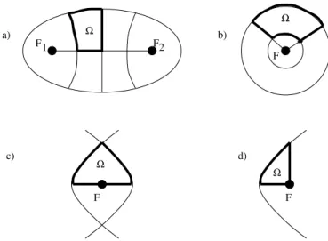
- in the case, when the common foci of the conics are distinct and finite (i.e., the conics are ellipses and (or) hyperbolas), the ambient line of each straight-line segment of the boundary is either the line through the foci, or the middle orthogonal line to the segment connecting the foci, see Fig. 1a); - in the case, when the conics are concentric circles, the above ambient lines may be any lines through their common center, see Fig. 1b);

- in the case, when the conics are confocal parabolas, the ambient line of each straight-line segment of the boundary is either the common axis of the parabolas, or the line through the focus that is orthogonal to the axis, see Fig. 1 c), d).

Let us extend the above definition to the non-Euclidean case. To do this, let us recall the following definition.

Definition 1.12 [46, p.84]. Let Σ ⊂ R3 be one of the standard surfaces of constant curvature defined by a quadratic form < Ax, x >. Let B be a real symmetric 3 × 3-matrix that is not proportional to A. In the Euclidean case, when A = diag(1, 1, 0), we require in addition that the x3-axis does

not lie in Ker B. The pencil of confocal conics in Σ defined by B consists of the conics

Γλ = Σ ∩ {< Bλx, x >= 0}, Bλ = (B − λA)−1. (1.1)

For those λ, for which det(B − λA) = 0 and the kernel Kλ = Ker(B − λA)

is one-dimensional, we set Γλ to be the geodesic3

Γλ= Σ ∩ Kλ⊥, (1.2)

provided that the latter intersection is non-empty. In the case, when dimKλ =

2, for every two-dimensional vector subspace H ⊂ R3 orthogonal to Kλ the

intersection Σ ∩ H will be also denoted Γλ = Γλ(H).

Remark 1.13 In the conditions of Definition 1.12 the confocal conic pencil is well-defined: det(B − λA) 6≡ 0 as a function of λ. In the non-Euclidean

3

Everywhere below, whenever the contrary is not specified, the orthogonal complement sign ⊥ and the vector product are understood with respect to the standard Euclidean scalar product on R3_.

(9)

cases this is obvious, since the matrix A is non-degenerate. In the Euclidean case one has A = diag(1, 1, 0) and the x3-axis does not lie in Ker B: that is,

some of the matrix elements B13, B23, B33 is non-zero. One has

det(B − λA) = −λ3det(A − λ−1B)

= λ2B33+ λ(B132 + B232 − B33(B11+ B22)) + det B 6≡ 0 : (1.3)

in the above right-hand side the identical vanishing of the coefficients at λ2 and at λ would imply that B33= B13= B23= 0, which is forbidden by our

assumptions. Hence, det(B − λA) 6≡ 0. Conversely, if in the Euclidean case the x3-axis were contained in the kernel of the matrix B, then obviously

det(B − λA) ≡ 0, and the confocal pencil would not be well-defined. Remark 1.14 The matrix B is uniquely defined modulo transformation B 7→ µB − λA, µ 6= 0 (i.e., modulo RA and up to constant factor) by the corresponding confocal pencil. In the Euclidean case, when Σ = {x3 = 1},

A = (1, 1, 0), the above notion of confocal conics coincides with the classical one. In the Euclidean case the kernel Kλ is two-dimensional for some λ, if

and only if the confocal conics under question are concentric circles; then the corresponding geodesics Γλ(H) are the lines through their common center.

Definition 1.15 Consider a confocal conic pencil (1.1) defined by a matrix B. The corresponding admissible geodesics are the following:

1) Each geodesic Γλ in (1.2) and (or) Γλ(H) (if any) is admissible.

2) Consider the special case, when B = Aa ⊗ b + b ⊗ Aa (modulo RA, see Remark 1.14) where a, b ∈ R3\ {0}, < a, b >= 0.

2a) In the subcase, when Σ is non-Euclidean: those of the geodesics {r ∈ Σ | < r, a >= 0}, {r ∈ Σ | < r, Ab >= 0} (1.4) that are well-defined (i.e., non-empty) are also admissible.

2b) In the subcase, when Σ = {x3 = 1} is Euclidean and b is not parallel

to Σ: only Γλ and the first geodesic in (1.4) are admissible.

Remark 1.16 Note that the subcase in 2) when Σ = {x3 = 1} and b is

parallel to Σ is impossible, since in this subcase the x3-axis would lie in

the kernel Ker B, which is forbidded by our assumptions. This implies that in subcase 2b) the first geodesic in (1.4) is non-empty: the vector a is not vertical, since its orthogonal b is not horizontal. In the above subcases 2a), 2b) the corresponding admissible geodesics from (1.4) do not coincide with geodesics Γλ (Γλ(H)). Indeed, suppose the contrary, say, the first geodesic

(10)

a⊥∩ Σ in (1.4) is non-empty and coincides with some Γλ or Γλ(H). Then

a ∈ Ker(B − λA), that is,

< Aa, a > b+ < b, a > Aa =< Aa, a > b = λAa.

Thus, either < Aa, a >= 0 and λAa = 0, or the vector b, which is orthogonal to a, is proportional to Aa, thus < Aa, a >= 0 again. But then a⊥∩ Σ = ∅, see [17, p.122], – a contradiction. The case, when the second geodesic in (1.4) coincides with Γλ, is treated analogously. The above non-coincidence

statement can be also deduced from the next proposition.

Remark 1.17 In the subcase 2a) set _ea = Ab, eb = Aa. Then B = A_ea ⊗ eb + eb ⊗ A_ea, and < _ea, eb >= 0, since A2 = Id. The geodesics in (1.4) are written in terms of the new vectors _ea and eb in the opposite order. Thus, each geodesic of type (1.4) can be represented by the first equation in (1.4) for appropriate presentation B = Aa ⊗ b + b ⊗ Aa.

Definition 1.18 A billiard Ω ⊂ Σ with a countably piecewise smooth boundary is countably confocal, if its boundary consists of arcs of confo-cal conics (at least one coniconfo-cal arc is present) and may be some segments of geodesics admissible with respect to the confocal conic pencil given by the conical arcs in ∂Ω, see Definition 1.15.

Confocal billiards with piecewise smooth boundaries were introduced by S.V.Bolotin [17], who proved their polynomial integrability with integrals of first, second or fourth degree. See the following proposition, whose proof presented in loc. cit. remains valid in the countably piecewise smooth case. Proposition 1.19 [17, proposition 1 in section 2; the theorem in section 4] Each countably confocal billiard is polynomially integrable: it has a non-trivial first integral that is either linear, or quadratic, or a degree 4 poly-nomial in the velocity components that is non-constant on the unit velocity hypersurface. If all the geodesic pieces of its boundary lie in Γλ (Γλ(H)),

then the integral can be chosen of degree at most 2. The case of a degree 4 integral that cannot be reduced to an integral of degree at most 2 is ex-actly the case, when the conics forming the billiard boundary are contained in a confocal pencil of types 2a) or 2b) from Definition 1.15 and the billiard boundary contains at least one segment of some of the admissible geodesics from (1.4) mentioned in 2a) and 2b) respectively.

(11)

F Ω F Ω Ω Ω F c) d) a) b) F F 1 2

Figure 1: Examples of confocal planar billiards; F1, F2, F are the foci;

the conics in c) and d) are parabolas. All of these billiards have quadratic integrals, except for the billiard at Fig. 1d), which has a degree 4 integral.

Example 1.20 For Euclidean billiards the two countably confocality no-tions given by Definino-tions 1.11 and 1.18 are equivalent. A Euclidean bil-liard whose boundary contains an arc of parabola and a segment of the line through the focus that is orthogonal to the axis of the parabola, as at Fig. 1d), is exactly a billiard of type 2b), see the end of paper [17]; the above line is the first geodesic in (1.4). This example of a billiard having a degree 4 integral was first discovered in [38]. Analogous billiards on surfaces of non-zero constant curvature were constructed in [2].

The main result of the paper is the following theorem.

Theorem 1.21 4 Let a billiard in Σ with countably piecewise C2-smooth boundary be polynomially integrable (or equivalently, analytically integrable, see Definition 1.2), and let the regular part of its boundary contain at least one non-geodesic arc. Then the billiard is countably confocal.

Theorem 1.21 is a joint result of M.Bialy, A.E.Mironov and the author. Its proof sketched below consists of the two following parts:

1) The papers [10, 11] of Bialy and Mironov, whose geometric construc-tion reduced the proof of Theorem 1.21 to a purely algebro-geometric

(12)

lem that was partially investigated by them.

2) The complete solution of the above-mentioned algebro-geometric prob-lem obtained in the present paper (Theorem 1.25).

1.2 Sketch of proof of Theorem 1.21 and plan of the paper

In what follows a point r ∈ Σ will be identified with its radius-vector in R3. Theorem 1.22 (S.V.Bolotin, see [16], [17, p.118; proposition 2 and its proof on p.119], [33, chapter 5, section 3, proposition 5].) For every polyno-mially integrable billiard Ω ⊂ Σ with countably piecewise C2-smooth bound-ary a polynomial integral non-constant on the unit velocity hypersurface {|P | = 1} can be chosen to be a homogeneous polynomial Ψ(M ) of even degree in the components of the moment vector

M = [r, P ] = (x2P3− x3P2, −x1P3+ x3P1, x1P2− x2P1), (1.5)

r = (x1, x2, x3) ∈ Σ, P = (P1, P2, P3) is the velocity vector.

(This statement is local and holds for reflection from an arbitrary smooth curve in Σ.) Each C2-smooth arc of the boundary ∂Ω with non-zero geodesic curvature lies in an algebraic curve.

Theorem 1.23 (see [17, section 4]). Let a billiard on Σ with a countably piecewise C2-smooth boundary be polynomially integrable. Let its boundary contain a non-geodesic conical arc. Then the billiard is countably confocal. Remark 1.24 S.V.Bolotin’s theorems implying Theorems 1.22 and 1.23 were stated and proved in loc. cit. for piecewise smooth boundaries, but their proofs remain valid in the countably piecewise smooth case. To make the paper self-contained and to extend the main results to complex domain, we give a proof of Theorem 1.23 in Subsection 2.2. It follows the arguments from [17, section 4], but here it is done in the dual terms using results of Bialy and Mironov from [10, 11].

The boundary ∂Ω is countably piecewise C2-smooth. Therefore, it con-tains an open and dense subset contained in ∂Ωreg that is a disjoint union

of geodesic segments and C2-smooth arcs with non-zero geodesic curvature. Let α ⊂ ∂Ω be a C2-smooth arc with non-zero geodesic curvature: it existence follows from assumptions. By Bolotin’s Theorem 1.23, for the proof of Theorem 1.21 it suffices to show that α contains a conical sub-arc.

(13)

To do this, we use Bialy–Mironov construction of the dual billiard and their results presented in Subsection 2.1. Let us describe them briefly.

In what follows π : R3_{\ {0} → RP}2 _{denotes the tautological projection.}

Its complexification and restriction to Σ will be also denoted by π.

Recall that the standard Euclidean scalar product < x, x > on R3defines the orthogonal polarity: the correspondence sending each two-dimensional vector subspace in R3 to its Euclidean-orthogonal one-dimensional sub-space. This together with the projection π induces a projective duality RP2∗(x1:x2:x3) → RP

2

(M1:M2:M3) sending lines to points. Namely, each

projec-tive line, which is the projection of a two-dimensional vector subspace H (punctured at the origin), is dual to the point π(H⊥\ {0}). (It is well-known that in the affine chart (x1: x2: 1) the projective duality defined by

the orthogonal polarity is the composition of the polar duality with respect to the unit circle and the central symmetry with respect to the origin.)

For simplicity, the curve dual to the projection π(α) ⊂ RP2 with respect to the above projective duality will be denoted by α∗ and called the curve Σ-dual to α. By definition, the dual curve α∗ is the family of points in RP2 that are dual to the projective tangent lines to the curve π(α) ⊂ RP2. The curve α∗ is C1-smooth, since the curve π(α) is C2-smooth and has no inflection points: the geodesic curvature of the curve α is non-zero.

Bialy and Mironov proved the following results in [10, 11]:

- Let Ψ(M ) be the homogeneous first integral of even degree 2n from Bolotin’s Theorem 1.22. For every point B ∈ α∗ the restriction to the projective tangent line TBα∗ of the rational function

G(M ) = Ψ(M )

< AM, M >n (1.6)

is invariant under a special projective involution TBα∗ → TBα∗ fixing B:

the so-called angular symmetry centered at B. More precisely, invariance of the function G is equivalent to the statement saying that for every r ∈ α the function Ψ(M ) = Ψ([r, v]) in v ∈ TrΣ is invariant under reflection of the

vector v from the line Trα.

- Consider the so-called absolute: the complex conic

I = {< AM, M >= 0} ⊂ CP2(M1:M2:M3). (1.7)

The above angular symmetry coincides with the restriction to TBα∗ of the

unique projective involution CP2 → CP2fixing B that fixes each line through B and permutes its intersection points with the conic I: the so-called I-angular symmetry centered at B.

(14)

- Concider the complex projective Zariski closure of the curve α∗, which is an algebraic curve, by Theorem 1.22. Each its non-linear irreducible com-ponent γ generates a rationally integrable I-angular billiard, see Definition 2.10: for every point B ∈ γ \ I the restriction of a rational function G to the projective tangent line TBγ is invariant under the I-angular symmetry

centered at B; the function G is non-constant on CP2 and has poles in I. - For every curve γ generating a rationally integrable I-angular billiard all its singular and inflection points (if any) lie in I.

The main algebro-geometric result of the present paper, which implies the main results, is the following theorem.

Theorem 1.25 Let I ⊂ CP2 be a conic: either regular, or a union of two distinct lines. Every irreducible algebraic curve γ ⊂ CP2 different from a line and from I and generating a rationally integrable I-angular billiard is a conic.

For the proof of Theorem 1.25 we study local branches of the curve γ at points C ∈ γ ∩ I: the irreducible components of the germ (γ, C). Each local branch is holomorphically bijectively parametrized in so-called adapted affine coordinates by small complex parameter t as follows:

t 7→ (tq, ctp(1 + o(1))), as t → 0; q, p ∈ N, 1 ≤ q < p, c 6= 0. In Section 4 we prove Theorem 4.1 giving a list of statements on p and q satisfied by local branches of appropriate type (see Cases 1) and 2) below). Afterwards in Section 5 we prove the following general algebro-geometric theorem. It states that Bialy–Mironov inclusions Sing(γ), Inf l(γ) ⊂ I and the statements of Theorem 4.1 on local branches together imply that γ is a conic.

Theorem 1.26 Let I ⊂ CP2 be a conic: either regular, or a union of two distinct lines. Let γ ⊂ CP2 be an irreducible complex algebraic curve differ-ent from a line and from I. Let all the singularities and inflection points (if any) of the curve γ lie in I. Let for every C ∈ γ ∩ I the local branches b of the curve γ at C satisfy the following statements:

Case 1): C is a regular point of the conic I. If b is tangent to I, then it is quadratic: p = 2q. If b is transversal to I, then it is regular and quadratic: q = 1, p = 2.

Case 2): I is a union of two distinct lines intersecting at C. If b is transversal to both lines, then b is subquadratic: p ≤ 2q.

(15)

The proof of Theorem 1.26, which will be given in Section 5, is based on the ideas and arguments due to E.Shustin on plane curve invariants from the proof of its analogue for the outer billiards case [27, subsections 4.1, 4.2]. The most technical part of the paper is the proof of statement (ii-b) of Theorem 4.1, which asserts that each local branch of the curve γ that is transversal to I and is based at a regular point of the conic I is regular and quadratic. Its proof is based on a remarkable formula of Bialy and Mironov for the Hessian of the function defining γ, see [10, theorem 6.1] and [11, formulas (16) and (32)]. This formula is recalled in Section 3 as formula (3.4). We use asymptotic formulas for both sides of Bialy–Mironov formula along the transversal local branches that are stated and proved in Subsection 3.4. In their proofs we use asymptotic formulas for the defining functions and their Hessians stated and proved in Subsections 3.2 and 3.3 respectively.

In Section 6 we prove the main results: Theorems 1.25, 1.21 and 1.6 and the complexification of Theorem 1.21 stated in the next subsection.

1.3 Complexification

Here we state a complexification of Theorem 1.21, which deals with the space C3(x1,x2,x3)equipped with a quadratic form < Ax, x >, x = (x1, x2, x3),

A ∈ {diag(1, 1, 0), diag(1, 1, ±1)}, and a complex surface Σ ⊂ C3_.

- Euclidean case: Σ = {x3 = 1}, A = diag(1, 1, 0).

- Non-Euclidean case: Σ = Σ±= {< Ax, x >= ±1}, A = diag(1, 1, ±1).

We equip the surface Σ under question with the complex bilinear quadratic form induced by the form < Ax, x > on its tangent planes.

Note that the surfaces Σ± are regular, connected and obtained one from

the other by the transformation (x1, x2, x3) 7→ (ix1, ix2, x3), but the latter

transformation changes the sign of the quadratic form < Ax, x > on T Σ±.

Recall that a one-dimensional subspace Λ in a complex linear space equipped with a C-bilinear scalar product is isotropic, if each vector in Λ has zero scalar square. A holomorphic curve Λ in a complex manifold Σ equipped with a C-bilinear quadratic form on T Σ is isotropic, if for every x ∈ Λ the tangent subspace TxΛ ⊂ TxΣ is isotropic.

A complex geodesic is

- a non-isotropic line in Σ = C2 in the Euclidean case;

- the intersection of the surface Σ with a two-dimensional subspace in C3 that is not tangent to the light cone bI = {< Ax, x >= 0} in the non-Euclidean case.

(16)

Proposition 1.27 Consider the non-Euclidean case: A = diag(1, 1, ±1). For every two-dimensional vector subspace H ⊂ C3 tangent to the light cone bI the intersection H ∩ Σ is a union of two parallel isotropic straight lines. Each isotropic holomorphic curve in Σ is a line contained in a two-dimensional vector subspace in C3 tangent to bI. For every r ∈ Σ the one-dimensional isotropic vector subspaces in the plane TrΣ are exactly its

in-tersections with two-dimensional vector subspaces in C3 containing r and tangent to bI: there are exactly two of them.

Proof For every r ∈ Σ the quadratic form on TrΣ induced by < Ax, x >

is non-degenerate, since TrΣ is < Ax, x >-orthogonal to the radius-vector

of the point r and transversal to it: < Ar, r >= ±1 6= 0. For every two-dimensional subspace H tangent to bI the restriction of the form < Ax, x > to H is non-zero and has a non-zero kernel K: the tangency line of the plane H with bI. Hence, in appropriate affine coordinates (z1, z2) on H centered at

0 one has < Ax, x > |H = z12, K = {z1 = 0}, H ∩Σ = {z12 = ±1}. Therefore,

the intersection H ∩ Σ is a union of two lines parallel to K, which are thus isotropic. The first statement of the proposition is proved.

Let us now prove the third and the second statements of the proposition. For every point r ∈ Σ the tangent plane TrΣ equipped with the quadratic

form induced by < Ax, x > contains two distinct one-dimensional isotropic vector subspaces, by non-degeneracy. Each ot them is the line of intersection of the plane TrΣ with a two-dimensional subspace H through r that is

tangent to bI. This follows from the first statement of the proposition and the fact that there are two distinct 2-dimensional subspaces through r that are tangent to bI. This implies the third statement of the proposition. This also implies that each isotropic curve in Σ is locally a phase curve of a (double-valued) holomorphic line field defined by the above intersections. The only phase curves of the latter field are the isotropic lines in H ∩ Σ, H being tangent to bI, by the first statement of the proposition and uniqueness theorem in ordinary differential equations. This proves the proposition. 2 Definition 1.28 Consider the surface Σ in the non-Euclidean case. Let γ ⊂ Σ be a complex geodesic. Let Gγ denote the stabilizer of the geodesic γ

in the group of automorphisms C3 → C3 _{preserving the form < Ax, x >. Its}

identity component, which will be denoted by G0_γ, will be called the group of translations along the geodesic γ. A translation of the complex Euclidean plane along a complex line L is the translation by a vector parallel to L. Remark 1.29 In the above definition in the non-Euclidean case let H ⊂ C3

(17)

denote the corresponding two-dimensional vector subspace: γ = H ∩ Σ. The geodesic γ is thus a regular conic in the plane H that is biholomorphically parametrized by C∗. Its projective closure ˆγ in CP2 ⊃ H intersects the infinity line CP2 \ H at two distinct points. The restrictions to γ of the translations along the geodesic γ are exactly those conformal automorphisms ˆ

γ → ˆγ that fix the latter intersection points. One has ˆγ ' C, γ ' C∗. This yields to a natural isomorphism G_γ0 ' C∗.

Definition 1.30 A complex billiard on Σ is a collection (finite or infinite, countable or uncountable) of holomorphic curves Γt ⊂ Σ distinct from

isotropic lines (see [25, definition 1.3] for finite collections in the Euclidean case). A complex billiard is said to be polynomially integrable, if there exists a function Φ(r, P ) on T Σ (called a polynomial integral) that is polynomial in P ∈ TrΣ with the following properties:

- Φ|{<AP,P >=1} 6≡ const;

- the restriction of the function Φ to the tangent bundle of every complex geodesic is invariant under the translations along the geodesic;

- for every point r ∈ Γt such that the line TrΓt is non-isotropic for

the quadratic form on TrΣ induced by < Ax, x > the restriction Φ|TrΣ is

invariant under the symmetry with respect to the complex line TrΓt(see [25,

definition 2.1]): the unique non-trivial C-linear involution TrΣ → TrΣ that

preserves the form < Ax, x > on TrΣ and fixes the points of the line TrΓt.

Example 1.31 Consider a polynomially integrable billiard with countably piecewise smooth boundary in a real surface of constant curvature. Then the smooth part of the boundary is contained in a union of arcs of conics and segments of admissible geodesics (Theorem 1.21). Their complexifications form a complex billiard having a polynomial integral that is the complexifi-cation of the real polynomial integral of the real billiard: it can be chosen of degree no greater than four, see Proposition 1.19.

Remark 1.32 The confocality notion from Definition 1.12 for real conics extends to the case of complex conics in Σ without changes in both non-Euclidean and non-Euclidean cases with B being a complex symmetric matrix and λ ∈ C. In the Euclidean case this complex confocality notion is equiv-alent to the one given in [25, definition 2.24], which follows from definition and Remark 1.14.

Remark 1.33 A pencil of confocal conics given by a matrix B is well-defined, if and only if inequality (1.3) holds: det(B − λA) 6≡ 0 as a function

(18)

of λ. In the real case inequality (1.3) is equivalent to the condition that the x3-axis is not contained in the kernel of the matrix B, i.e., (B13, B23, B33) 6=

(0, 0, 0), see Remark 1.13. In the complex case inequality (1.3) is equivalent to the following weaker condition: for every choice of sign ± the equalities

B33= 0, B23= ±iB13, B132 (B11− B22± 2iB12) = 0

do not hold simultaneously.

Definition 1.34 A complex billiard Γt is said to be confocal, if the set of

its curves different from complex geodesics is non-empty, all of them are confocal complex conics, and the complex geodesics from the family Γt are

admissible with respect to the corresponding confocal conic pencil in the sense of Definition 1.15, where now everything is complex: B, λ, a, b,... Remark 1.35 A priori, some complex curves Γλ in (1.2), Γλ(H) and some

subsets in (1.4) may be isotropic lines; then they are not complex geodesics, and we do not call them admissible. For example, in the non-Euclidean case let λ ∈ C be such that the kernel Kλ= Ker(B −λA) is one-dimensional. The

corresponding intersection Γλ = Kλ⊥∩ Σ is isotropic, if and only if Kλ ⊂ bI. This follows from Proposition 1.27 and since the Euclidean orthogonal K_λ⊥ is tangent to the light cone bI if and only if Kλ ⊂ bI: see the last statement of Corollary 2.15 in Subsection 2.2.

Theorem 1.36 Every polynomially integrable complex billiard Γton Σ

con-taining at least one non-geodesic curve is confocal and has an integral Φ(r, P ) = Ψ(M ) (where M = [r, P ] is the complexified Euclidean vector product) that is a homogeneous polynomial in M of degree at most four. The integral can be chosen quadratic in M , except for the cases 2a), 2b) in Definition 1.15, when Γt contains a corresponding admissible complex geodesic of type (1.4):

in this case there is an integral of degree four. Theorem 1.36 will be proved in Subsection 6.4.

1.4 Historical remarks

Existence of caustics in any strictly convex planar billiard with sufficiently smooth boundary was proved by V.F.Lazutkin [34]. Non-existence of caus-tics in higher-dimensional billiards with boundaries different from quadrics was proved by M.Berger [6].

The Birkhoff Conjecture was studied by many mathematicians. In 1950 H.Poritsky [37] proved it under the additional assumption that the billiard

(19)

in each closed caustic near the boundary has the same closed caustics, as the initial billiard. Later in 1988 another proof of the same result was obtained by E.Amiran [5]. Recall that the reflection from the boundary of a convex planar billiard Ω acts on the space of oriented lines intersecting Ω, and their space is called the phase cylinder: each line is reflected from the boundary ∂Ω at its last point of intersection with ∂Ω (with respect to its orientation), and its reflected image is directed inside the domain Ω at this point. In 1993 M.Bialy [7] proved that if the phase cylinder of the billiard is foliated by non-contractible continuous closed curves which are invariant under the billiard map, then the boundary ∂Ω is a circle. (Another proof of the same result was later obtained in [47].) In particular, Bialy’s result implies Birkhoff Conjecture under the assumption that the foliation by caustics extends to the whole billiard domain punctured at one point: then the boundary is a circle. In 2012 he proved a similar result for billiards on the constant curvature surfaces [8] and also for magnetic billiards [9]. In 1995 A.Delshams and R.Ramirez-Ros suggested an approach to prove splitting of separatrices for generic perturbation of ellipse [19]. In 2013 D.V.Treschev [42] made a numerical experience indicating that there should exist analytic locally integrable billiards, with the billiard reflection map having a two-periodic point where the germ of its second iterate is analytically conjugated to a disk rotation. Recently Treschev studied the billiards from [42] in more detail in [43] and their multi-dimensional versions in [44]. A similar effect for a ball rolling on a vertical cylinder under the gravitation force was discovered in [3]: the authors have shown that the ratio between its vertical and horizontal oscillation periods is a universal irrational constant, the number p7/2. Recently V.Kaloshin and A.Sorrentino have proved a local version of the Birkhoff Conjecture [31]: an integrable deformation of an ellipse is an ellipse. (The case of ellipses with small extentricities was treated in the previous paper by A.Avila, J. De Simoi and V.Kaloshin [4].) A dynamical entropic version of Birkhoff Conjecture was stated and partially studied by J.-P.Marco in [35].

In 1988 A.P.Veselov proved that every billiard bounded by confocal quadrics in any dimension has a complete system of first integrals in in-volution that are quadratic in P [45, proposition 4]. In 1990 he studied a billiard in a non-Euclidean ellipsoid: in the sphere and in the Lobachevsky (i.e., hyperbolic) space of any dimension n. He proved its complete inte-grability and provided an explicit complete list of first integrals [46, the corollary on p. 95]. In the same paper he proved that all the sides of a billiard trajectory are tangent to the same n − 1 quadrics confocal to the boundary of the ellipsoid and the billiard dynamics corresponds to a shift of

(20)

the Jacobi variety corresponding to an appropriate hyperelliptic curve [46, theorems 3, 2 on p. 99]. The Polynomial Birkhoff Conjecture together with its generalization to surfaces of constant curvature was stated and studied by S.V.Bolotin, who proved in 1990 that in its conditions the billiard bound-ary lies in an algebraic curve [16]. In the same paper and in [17, section 4] he proved the conjecture under the assumption that at least one irreducible component of the corresponding complex projective planar algebraic curve is non-linear and nonsingular (in the non-Euclidean case it is also required that in addition, at least one intersection point of the latter component with the absolute be transversal). In [17] Bolotin proved integrability of countably confocal billiards with piecewise smooth boundaries with integrals of degrees two or four and a similar statement in higher-dimensional spaces of constant curvature. M.Bialy and A.E.Mironov proved the planar Polynomial Birkhoff Conjecture in the case of integrals of degree four [12]. A version of the pla-nar Polynomial Birkhoff Conjecture for families of billiards sharing the same polynomial integral (with boundaries depending continuously on one param-eter) was solved in [1]: in loc. cit. it is sufficient to require that the union of the boundaries do not lie in an algebraic curve in R2, see [1, end of p.30]. Dynamics in countably confocal billiards with piecewise smooth boundaries in two and higher dimensions was studied in [20, 21, 22, 23, 24]. Dynamics in the so-called pseudo-integrable billiards (more precisely, confocal billiards with non-convex angles) was studied in [21, 22, 23, 24]. For further results on the Polynomial Birkhoff Conjecture and its version for magnetic billiards see the above-mentioned papers [10, 11, 12] by M.Bialy and A.E.Mironov, [13, 14] and references therein.

The analogue of the Birkhoff Conjecture for outer billiards was stated by S.L.Tabachnikov [41] in 2008. Its polynomial version was stated by Tabach-nikov and proved by himself under genericity assumptions in the same paper, and recently solved completely in the joint work of the author of the present paper with E.I.Shustin [27].

2 Preliminaries: from polynomially integrable to

I-angular billiards

2.1 _{Reflection and I-angular symmetry}

Here we present results of M.Bialy and A.E.Mironov mentioned in Subsec-tion 1.2 and give self-contained proofs of some of them.

(21)

Proposition 2.1 (S.V.Bolotin, see [17, formula (15), p.23], [33, formula (3.12), p.140]). For every r ∈ Σ the linear operator Mr : TrΣ → Vr = r⊥,

v 7→ [r, v] is an isomorphism preserving the quadratic form < Ax, x >. Here the orthogonal complement and the vector product are taken with respect to the standard Euclidean scalar product, see Footnote 3.

Definition 2.2 Let the space Rn _{be equipped with a quadratic form <}

Ax, x >, A being a symmetric n × n-matrix, and let ` ⊂ Rn be a one-dimensional vector subspace such that ` 6⊂ {< Ax, x >= 0}. The pseudo-symmetry of the space Rn _{with respect to the line ` is the linear involution}

Rn→ Rn preserving the quadratic form, fixing the points of the line ` and acting as central symmetry in its orthogonal complement with respect to the form. The definition of complex pseudo-symmetry of the space Cnequipped with a C-bilinear quadratic form is analogous.

Corollary 2.3 For every r ∈ Σ and one-dimensional subspace ` ⊂ TrΣ

the mapping Mr : TrΣ → Vr, v 7→ M conjugates the pseudo-symmetry

TrΣ → TrΣ with respect to the line ` and the pseudo-symmetry Vr → Vr

with respect to the one-dimensional subspace orthogonal to both r and `. Definition 2.4 Let I ⊂ CP2 be a conic: either a smooth conic, or a union of two distinct lines. Let B ∈ CP2\ I. For every complex line L through B consider its complex projective involution fixing B and permuting its in-tersection points with I. (If L is tangent to I, the involution under question is the unique non-trivial projective involution L → L fixing B and the tan-gency point.) The transformation thus constructed for each L is a projective involution CP2 → CP2_{fixing B, which will be called the I-angular symmetry}

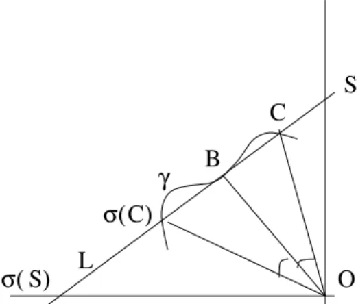
with center B. See Fig. 2 in the Euclidean case.

Proposition 2.5 Consider the space C3_(M₁_,M₂_,M₃₎equipped with a quadratic form < AM, M >, dim(Ker A) ≤ 1. The absolute I = {< AM, M >= 0} ⊂ CP2_(M₁_:M₂_:M₃₎, see (1.7), is either a regular conic, or a union of two distinct lines. The projectivization of a pseudo-symmetry C3→ C3 _{with respect to a}

one-dimensional subspace ` is the I-angular symmetry with center π(`). The proposition follows from definition.

Theorem 2.6 (see [11, theorem 1.3, p.151] in the non-Euclidean case). Let Ω ⊂ Σ be a polynomially integrable billiard with countably piecewise smooth boundary and a homogeneous polynomial integral Ψ(M ) of even degree. Let r be a point in a smooth arc in ∂Ω. Set Vr = r⊥ ⊂ R3. Let L ⊂ Vr be the

(22)

σ( )

O

γ

S

L

σ( )

S

B

C

Figure 2: The I-angular symmetry σ : CP2 → CP2 with center B in the Euclidean case, when I = {x21 + x22 = 0}: the action in the affine chart

C2_(x₁_,x₂₎; O = (0, 0). The lines OC and Oσ(C) are symmetric with respect to the line OB. The projective lines OS and Oσ(S) are isotropic for the complex Euclidean metric dx2₁+ dx2₂ on C2, that is, I = OS ∪ Oσ(S).

one-dimensional subspace Euclidean-orthogonal to both r and the tangent line Tr∂Ω. The restriction Ψ|Vr is invariant under the pseudo-symmetry of

the plane Vr equipped with the form < Ax, x > with respect to the line L.

Proof The polynomial integral Ψ([r, v]) is invariant under the action on v of the pseudo-symmetry TrΣ → TrΣ with respect to the line ` = Tr∂Ω

(invariance under reflection). This together with Corollary 2.3 implies the

statement of the theorem. 2

Convention 2.7 Recall that for every C2-smooth curve α ⊂ Σ with non-zero geodesic curvature its Σ-dual is the curve α∗ ⊂ RP2

orthogonal-polar-dual to the projection π(α) ⊂ RP2, see Subsection 1.2. For every r ∈ Σ each one-dimensional vector subspace ` ⊂ TrΣ is the intersection of the

tangent plane TrΣ with a two-dimensional subspace H ⊂ R3 containing

r. The intersection b` = H ∩ Σ is the geodesic tangent to `. The point π(H⊥\ {0}) ∈ RP2 will be called the point Σ-dual to the subspace ` and to the geodesic b`. It will be denoted by b`∗.

Theorem 2.8 Let Ω ⊂ Σ be a polynomially integrable billiard with a count-ably piecewise C2-smooth boundary. Let Ψ(M ) be its homogeneous polyno-mial integral of even degree 2n. The function G = _{<AM,M >}Ψ(M ) n from (1.6)

(23)

treated as a rational function on CP2(M1:M2:M3) satisfies the following

state-ments.

1) For every C2_{-smooth arc α ⊂ ∂Ω with non-zero geodesic curvature,}

let α∗ ⊂ RP2 be its Σ-dual curve, for every point C ∈ α∗ the restriction of the function G to the projective line TCα∗ is invariant under the I-angular

symmetry with center C. One has G|α∗ ≡ const.

2) For every geodesic b` ⊂ Σ that contains a segment of the boundary ∂Ω the function G is invariant under the I-angular symmetry of the whole projective plane CP2 with center b`∗: the point Σ-dual to b`.

Remark 2.9 A version of statement 1) of Theorem 2.8 in the Euclidean case was proved in [10, theorem 3] for convex domains with smooth boundary. But its proof remains valid in the general Euclidean case.

Proof of Theorem 2.8. Each point C ∈ α∗ is dual to the projective line tangent to the curve π(α) at some point π(r), r ∈ α, by definition. Consider the projective line TCα∗ and set V = π−1(TCα∗) ∪ {0} ⊂ R3. It is

the two-dimensional subspace orthogonal to the line Or, by definition. Set L = π−1(C) ∪ {0} ⊂ V : it is the one-dimensional subspace orthogonal to both lines Trα and Or, by definition. The restrictions to V of both functions

Ψ(M ) and < AM, M > are invariant under the pseudo-symmetry of the plane V with respect to the line L, by Theorem 2.6 and isometry. Hence, the restriction to V of the ratio G(M ) = _{<AM,M >}Ψ(M ) n is also invariant. Therefore,

the restriction to π(V \ {0}) = TCα∗ of the function G treated as a rational

function on CP2is invariant under the projectivized pseudo-symmetry, which coincides with the I-angular symmetry centered at C, by Proposition 2.5. The equality G|α∗ ≡ const holds since the derivative of the function G at C

along a vector tangent to TCα∗vanishes. Indeed, the function G|TCα∗, which

is invariant under a projective involution fixing C, has zero derivative at C, similarly to vanishing of derivative of an even function at 0. Statement 1) is proved. The proof of statement 2) is analogous. In more detail, let Λ ⊂ Σ be a geodesic whose segment I ⊂ Λ is contained in ∂Ω. For every point Q ∈ I the projective line Q∗ dual to π(Q) passes through the point Λ∗Σ-dual to Λ. The restriction G|Q∗ is invariant under the I-angular symmetry with center

Λ∗, as in the above argument. Therefore, this holds for the restriction of the function G to every complex line through Λ∗, and hence, on all of CP2, by uniqueness of analytic extension. Statement 2) is proved. 2 Definition 2.10 Let I ⊂ CP2be a conic: either a regular conic, or a pair of distinct lines. Let γ ⊂ CP2 be an irreducible algebraic curve different from

(24)

a line and from I. We say that γ generates a rationally integrable I-angular billiard, if there exists a non-constant rational function G on CP2 with poles contained in I (called the integral of the I-angular billiard) such that for every C ∈ γ \ I the restriction of the function G to the projective tangent line TCγ is invariant under the I-angular symmetry with center C.

Corollary 2.11 Let I ⊂ CP2(M1:M2:M3)be the absolute, see (1.7). Let Ω ⊂ Σ

be a polynomially integrable billiard with a non-trivial homogeneous integral Ψ(M ) of even degree 2n. Let α ⊂ ∂Ω be a C2-smooth arc with non-zero geodesic curvature, and let α∗ ⊂ RP2 _{⊂ CP}2 _{be its Σ-dual curve. The}

complex projective Zariski closure of the curve α∗ is an algebraic curve. Each its non-linear irreducible component generates a rationally integrable I-angular billiard with integral G(M ) = _{<AM,M >}Ψ(M ) n, see (1.6).

Proof The function G is non-constant on CP2, since Ψ|{<AM,M >=1} 6≡

const: the latter statement follows from non-constance of the function Ψ([r, v]) on the hypersurface {< Av, v >= 1} (non-triviality of the integral) and Proposition 2.1. The first statement of the corollary, which follows from Bolotin’s Theorem 1.22, also follows from constance of the function G on α∗, see Statement 1) of Theorem 2.8. Its second statement follows from the invariance of the function G in Statement 1) of Theorem 2.8 by

straightfor-ward analytic extension argument. 2

Proposition 2.12 Let an irreducible algebraic curve γ ⊂ CP2 generate a rationally integrable I-angular billiard with the integral G. Then G|γ ≡

const.

The proof of the proposition repeats literally the above proof of the analogous statement from Theorem 2.8, part 1).

2.2 _{Duality and I-angular billiards. Proof of Theorem 1.23}

For the proof of Theorem 1.23 we use the well-known classical properties of the orthogonal polarity given by the following proposition and its corollary. We present the proof of the proposition for completeness of presentation. Proposition 2.13 Let B be a non-degenerate complex symmetric 3 × 3-matrix. Consider the complex space C3 with coordinates x = (x1, x2, x3)

equipped with the complex-bilinear Euclidean quadratic form dx2₁+dx2₂+dx2₃. The complex orthogonal-polar-dual to the conic in CP2(x1:x2:x3) given by the

(25)

Proof Consider the cone K = {x ∈ C3 \ {0} | < Bx, x >= 0} and its tautological projection Γ = π(K) ⊂ CP2, which is the conic under consider-ation. Let x ∈ K. The projective tangent line L = T_π(x)Γ is defined by the tangent plane TxK considered as a vector subspace in C3. It follows from

definition that TxK consists of those vectors v for which < Bx, v >= 0.

Thus, (TxK)⊥ = C(Bx), and the dual L∗ is π(Bx). Therefore, the dual

Γ∗ is the projection π(B(K)), which is obviously defined by the equation < B(B−1y), B−1y >=< B−1y, y >= 0. This proves the proposition. 2 Definition 2.14 [46, p.84]. Let A, B be two real non-proportional sym-metric 3 × 3-matrices. They define a pseudo-Euclidean pencil of conics in RP2: the conics given by the equation

{< (B − λA)M, M >= 0} ⊂ RP2(M1:M2:M3), λ ∈ R.

The same pencil of complex conics in CP2 depending on λ ∈ C will be also called pseudo-Euclidean.

Corollary 2.15 The Σ-duality transforms every confocal pencil of conics to the corresponding pseudo-Euclidean pencil. Namely, for every real sym-metric 3 × 3-matrix B satisfying the conditions of Definition 1.12 for any two conics in Σ lying in the confocal pencil (1.1) defined by B their Σ-dual curves lie in conics belonging to the pseudo-Euclidean pencil defined by the same matrix B. In the non-Euclidean case, when the absolute I is a regular conic, I is self-dual with respect to complex orthogonal polarity.

The first statement of the corollary is obvious. The self-duality follows from Proposition 2.13 and involutivity: A2 = Id in the non-Euclidean case. Proof of Theorem 1.23. Let Ω ⊂ Σ be a polynomially integrable billiard. Let Ψ(M1, M2, M3) be a non-trivial homogeneous polynomial integral of

the billiard Ω of even degree 2n. Consider the affine chart M3 6= 0 on

CP2(M1:M2:M3) with coordinates (x, y): x =

M1

M3, y =

M2

M3. Set

Q(x, y) =< AM, M >, where M = (x, y, 1) :

Q(x, y) = x2+ y2 in the Euclidean case; otherwise Q(x, y) = x2+ y2± 1. In this affine chart the function G on CP2 from (1.6) takes the form

G(x, y) = F (x, y)

(26)

In what follows for every conic α ⊂ Σ the corresponding complex conic containing its Σ-dual α∗ will be denoted by α_e∗.

Let the boundary ∂Ω contain an arc of a conic α. Let C denote the confocal conic pencil containing α, and let C∗ denote the corresponding (Σ-dual) pseudo-Euclidean pencil of conics containingα_e∗:

κλ= {< BλX, X >= 0} ⊂ R3(X1,X2,X3), Bλ = (B − λA) −1 , Cλ = κλ∩ Σ; κ∗_λ= {< (B − λA)M, M >= 0} ⊂ C3(M1,M2,M3), C ∗ λ= π(κ ∗ λ\ {0}) ⊂ CP2, κ∗_∞= bI = {< AM, M >= 0} ⊂ C3, C∞∗ = π(κ∗∞\ {0}) = I.

Claim 1. Each C2-smooth arc of the boundary ∂Ω with non-zero geodesic curvature lies in a conic confocal to α.

Proof The conic α_e∗ generates a rationally integrable I-angular billiard with integral G, by Corollary 2.11. On the other hand, it is known that the billiard on a conic α admits a non-trivial quadratic homogeneous first integral eΦ = eΦ(M ), see [17, proposition 1]. Set

e

F (x, y) = eΦ(x, y, 1), eG(x, y) = F (x, y)e Q(x, y).

Claim 2. The level curves of the function eG are conics from the pencil C∗, and the function G is constant on each of them.

Proof For every conic β confocal to α the quadratic integral eΦ is also an integral for the billiard on the conic β. This is well-known, see [17], and follows from the explicit formula [17, formula (12)] for the quadratic integral. Therefore, both corresponding complexified dual conicsα_e∗ and eβ∗ generate rationally integrable I-angular billiards with a common quadratic rational integral eG having first order pole at I, by Corollary 2.11. Hence,

e

G is constant on α_e∗ and eβ∗, by Proposition 2.12. Thus, the integral eG is constant on every conic from the complex pseudo-Euclidean pensil C∗, since the above conics eβ∗ with β being confocal to α form a real one-dimensional subfamily in C∗. Let us normalize the integral eG by additive constant (or equivalently, the integral eΦ by addition of c < AM, M >, c = const) so that eG|

e

α∗ ≡ 0. After this normalization one has eF |

e

α∗ ≡ 0: that is, eF

is the quadratic polynomial defining the conic α_e∗. On the other hand, α_e∗ generates a rationally integrable I-angular billiard with integral G (Corollary 2.11). Hence, G|

e

α∗≡ c₁= const, by Proposition 2.12. Therefore,

(27)

G1(x, y) =

f1(x, y)

(Q(x, y))n−1, deg f1 ≤ 2n − 2.

Hence, the fraction G1 is also a rational integral of the I-angular billiard

generated byα_e∗, as are G and eG. Thus, G1|α_e∗ ≡ c₂ = const, by Proposition

2.12. Similarly we get that

G1(x, y) = c2+ G2(x, y) eG(x, y), G2(x, y) =

f2(x, y)

(Q(x, y))n−2,

deg f2 ≤ 2n − 4, and G2 is an integral of the I-angular billiard generated

by αe

∗_{, as are G}

1 and eG. Continuing this prodecure we get that G is a

polynomial in eG. Hence, G ≡ const on the level curves of the function eG, that is, on the conics from the pencil C∗. Claim 2 is proved. 2 Let φ be a C2-smooth arc in ∂Ω with non-zero geodesic curvature, and let φ∗ ⊂ RP2 ⊂ CP2 denote its Σ-dual curve. The curve φ∗ lies in a level curve of the function G, by Theorem 2.8, statement 1). Hence, it lies in a finite union of conics from the pencil C∗, since each level curve of the function G is a finite union of conics in C∗ (follows from Claim 2). Therefore, φ lies in just one conic confocal to α, by smoothness, since any two intersecting

confocal conics are orthogonal. This proves Claim 1. 2

Now it remains to show that if ∂Ω contains geodesic segments, then their ambient geodesics are admissible with respect to the pencil C, see Definition 1.15. As it is shown below, this is implied by the following proposition. Proposition 2.16 Let B be a real symmetric 3 × 3-matrix as in Definition 1.12. Let C denote the corresponding pencil (1.1) of confocal conics in Σ. The corresponding admissible geodesics in Σ from Definition 1.15 are exactly those geodesics bl, for which the symmetry of the surface Σ with respect to bl leaves the pencil C invariant: the symmetry permutes confocal conics. Or equivalently, the geodesics bl for which the I-angular symmetry with center bl∗ Σ-dual to bl leaves the Σ-dual pseudo-Euclidean pencil C∗ invariant.

Remark 2.17 We will be using only the second statement of Proposition 2.16 characterizing admissible geodesics bl in terms of I-angular symmetry with center bl∗of the pencil C∗. Their characterization in terms of symmetry of the pencil C will be proved just for completeness of presentation.

Proof of Proposition 2.16. Let us first prove that for every given geodesic bl ⊂ Σ the two statements of the proposition are indeed equiva-lent. As it is shown below, this is implied by the following proposition.

(28)

Proposition 2.18 Consider the action of the symmetry with respect to a given geodesic bl ⊂ Σ on the space of all the geodesics in Σ. The Σ-duality conjugates this action to the I-angular symmetry with center bl∗.

Proof It suffices to prove the above conjugacy on the space of those geodesics that intersect bl, by analyticity and since they form an open sub-set in the connected manifold of geodesics. Each geodesic through a point r ∈ bl is uniquely determined by its tangent line: a one-dimensional subspace Λ ⊂ TrΣ. Thus, it suffices to show that the Σ-duality conjugates the

sym-metry action on the projectized tangent plane P(TrΣ) with the I-angular

symmetry centered at bl∗. Indeed, the Σ-duality sends each one-dimensional subspace Λ ⊂ TrΣ to the point bΛ∗∈ RP2represented by the one-dimensional

vector subspace Λr ⊂ R3 _{orthogonal to both r and Λ (see Convention 2.7).}

The linear isomorphism Mr : TrΣ → Vr = r⊥, v 7→ [r, v] sends each

sub-space Λ to Λr and conjugates the pseudo-symmetries with respect to the lines Trbl ⊂ T_rΣ and (T_rbl)r⊂ V_r, by definition and Corollary 2.3. Therefore, its projectivization realizes the Σ-duality P(TrΣ) → P(Vr) and conjugates

the action of the symmetry with respect to the line Trbl on the source with the projectivized pseudo-symmetry of the image: the I-angular symmetry with center bl∗ = π((Trbl)r) (Proposition 2.5). Proposition 2.18 is proved. 2 Note that for every curve γ ⊂ Σ the Σ-duality sends the family of geodesics tangent to γ to the Σ-dual curve γ∗ (see Convention 2.7). This to-gether with the above proposition implies equivalence of the two statements of Proposition 2.16. Thus, it suffices to prove its second statement: those geodesics bl, for which the pseudo-Euclidean pencil C∗ is invariant under the I-angular symmetry with center bl∗, are exactly the admissible geodesics from Definition 1.15.

Fix a geodesic bl. Let H ⊂ R3denote the two-dimensional vector subspace containing bl. Fix a vector a ∈ H⊥_{⊂ R}3_{, a 6= 0. It represents the Σ-dual b}_l∗ ₌

π(a). The vector a lies in a unique cone κ∗_λwith λ 6= ∞, since < Aa, a >6= 0: otherwise, if < Aa, a >= 0, then the intersection bl = H ∩ Σ would be empty. Indeed, in the Euclidean case the equality < Aa, a >= 0 on a real vector a holds exactly when a lies in the x3-axis; then H is parallel to the plane Σ,

H ∩ Σ = ∅. In the non-Euclidean case the equality < Aa, a >= 0 implies that A = diag(1, 1, −1) and the projective line a∗ = π(H \ {0}) is tangent to the real absolute {< Ax, x >= 0} ⊂ RP2(x1:x2:x3), by self-duality (Corollary

2.15). Then H is tangent to the cone {< Ax, x >= 0} ⊂ R3 and hence, it is disjoint from the inner component containing Σ of the complement of the latter cone. Thus, H ∩ Σ = ∅, – a contradiction.

(29)

Without loss of generality we will consider that a ∈ κ∗₀, after replacing B by B − λA for appropriate λ, by the inequality < Aa, a >6= 0. Let S : C3 _{→ C}3 _{denote the pseudo-symmetry with respect to the line Ca.}

Claim 3. The pseudo-Euclidean pencil C∗ is invariant under the I-angular symmetry with center bl∗, if and only if S(κ∗₀) = κ∗₀.

Proof The above I-angular symmetry is the projectivization of the pseudo-symmetry S. Therefore, invariance of the pencil C∗ under the I-angular symmetry is equivalent to the S-invariance of the family of cones κ∗_λ, that is, to the existence of an involution h : λ → h(λ) such that S(κ∗_λ) = κ∗_h(λ). In the latter case one has S(κ∗₀) = κ∗₀, since S(a) = a, a ∈ κ∗₀ and a /∈ κ∗_λ for every λ 6= 0. Conversely, let S(κ∗₀) = κ∗₀. This means that the involution S sends the quadratic form < Bx, x > to itself up to sign. Hence, S(κ∗_λ) = κ∗_±λ for every λ, since S preserves the quadratic form < AX, X >. This together with the previous equivalence statement proves the claim. 2 Claim 4. One has S(κ∗₀) = κ∗₀, if and only if κ∗₀ is a union of a pair of 2-planes through the origin in C3 that has one of the following types:

α) both planes contain the line Ca (they may coincide);

β) one plane in κ∗₀ contains the line Ca, and the other plane coincides with the two-dimensional subspace HA⊂ C3 that is orthogonal to the vector

a with respect to the scalar product < Ax, x >.

Proof Every hyperplane W ⊂ C3 parallel to the plane HA is S-invariant,

and S acts there as the central symmetry with respect to the point CW

of intersection W ∩ (Ca). The S-invariance of the cone κ∗0 is equivalent to

the invariance of each intersection IW = W ∩ κ∗0 under the latter symmetry

for every W as above. The intersection IW is either all of W , or a line

through CW, or a conic in W containing the center of its symmetry CW,

since Ca ⊂ κ∗0. In the latter case IW is a union of two lines through CW,

since a planar conic central-symmetric with respect to some its point C is a union of two lines through C (the lines under question may coincide). Note that all the intersections IW with W 6= HA are naturally isomorphic

between themselves via homotheties centered at the origin, since κ∗₀ is a cone. Therefore, the following two cases are possible.

α) IW is a union of two (may be coinciding) lines through CW for every

W ; then κ∗₀ is a union of two planes containing the line Ca.

β) IW is a line for all W 6= HA, and IW = W for W = HA; then κ∗0 is a

union of the plane HA and another plane containing Ca.

This proves the claim. 2

(30)

invariant under the I-angular symmetry centered at bl∗; or equivalently, the cone κ∗₀ = {< Bx, x >= 0} be a union of two planes, as in Claim 4.

Case α). The above planes both contain a, thus a ∈ Ker B; dim(Ker B) = 1, if the planes are distinct; dim(Ker B) = 2, if they coincide. Hence, the hyperplane H orthogonal to a with respect to the standard Euclidean scalar product is orthogonal to Ker B. Therefore, the geodesic bl = H ∩ Σ is ad-missible of type 1) in Definition 1.15. Vice versa, each adad-missible geodesic of type 1) can be represented as above after replacing B by B − λA.

Case β). Then the cone κ∗₀ is the union of the plane HA and a plane Π

containing the line Ca. The plane Π is the complexification of a real plane, which will be here also denoted by Π, since κ∗₀ is defined by a quadratic equation over real numbers and HA is the complexification of a real plane.

Let b ∈ R3 \ {0} denote a vector Euclidean-orthogonal to Π. Thus, < a, b >= 0. Note that the vector Aa is non-zero, since < Aa, a >6= 0, as was shown above, and it is Euclidean-orthogonal to HA, by definition. Therefore,

< BM, M >= c < Aa, M >< b, M >, c ∈ R \ {0}. Let us normalize the vectors a and b by constant factors so that c = 2. Then the quadratic form < BM, M > can be represented in the tensor form as Aa ⊗ b + b ⊗ Aa. The plane H defining the geodesic bl is the plane orthogonal to the vector a, by definition. Hence, bl is an admissible geodesic of type 2) in Definition 1.15: the first geodesic in (1.4). Vice versa, each geodesic of type 2) can be represented as above, see Remark 1.17. Proposition 2.16 is proved. 2 Let now bl ⊂ Σ be a geodesic whose some segment is contained in the boundary of the polynomially integrable billiard under question. The I-angular symmetry with center bl∗ leaves invariant the rational integral G, by Theorem 2.8. Hence, it permutes the level curves of the quadratic rational function eG, and the pencil C∗ is invariant, by Claim 2. Thus, the geodesic bl is admissible, by Proposition 2.16. Theorem 1.23 is proved. 2

3 Bialy–Mironov Hessian Formula and asymptotics

of Hessians

The material of the present section will be used in Section 4 in the proof of Theorem 4.1, statement (ii-b). It includes:

- Bialy–Mironov Hessian Formula (3.4) recalled in Subsection 3.1; - the asymptotics of its left- and right-hand sides along those local branches of the curve γ that are transversal to I (Subsection 3.4).

(31)

- for the defining function of an irreducible germ a of analytic curve along another irreducible germ b (Subsection 3.2);

- for the Hessian H(f ) of defining function of a given germ b along b (Subsection 3.3).

3.1 Bialy–Mironov formula

Let γ ⊂ CP2 be an irreducible algebraic curve generating a rationally inte-grable I-angular billiard with integral G. The function G has poles contained in I and is constant on γ, by Proposition 2.12. In what follows we normalize it so that G|γ ≡ 0, and set

Γ = {G = 0} ⊃ γ.

Fix an affine chart C2⊂ CP2with coordinates (x, y) such that the infinity line is not contained in I. In this chart the function G takes the form

G(x, y) = F1(x, y)

(Q(x, y))n, where F1 is a polynomial of degree at most 2n,

Q(x, y) is a fixed quadratic polynomial defining I : I = {Q = 0}. Let f (x, y) be the polynomial defining the curve γ, which is irreducible, as is γ: γ = {f = 0}, the differential df being non-zero on a Zariski open subset in γ. Recall that the polynomial F1 vanishes on γ. Therefore,

F1 = fkg1, k ∈ N, g1 is a polynomial coprime with f. (3.1)

Set g = g 1 k 1, F = F 1 k 1 = f g, m = n k. (3.2)

We consider the Hessian quadratic form of the function f (x, y) evaluated on appropriately normalized tangent vector to γ = {f = 0} at a point (x, y), namely, the skew gradient (fy, −fx) with respect to the standard complex

symplectic form dx ∧ dy:

H(f ) = fxxfy2− 2fxyfxfy+ fyyfx2. (3.3)

Theorem 3.1 (see, [10, theorem 6.1], [11, formulas (16) and (32)]) The following formula holds for all (x, y) ∈ γ:

On polynomially integrable Birkhoff billiards on surfaces of constant curvature.

HAL Id: ensl-01664204

https://hal-ens-lyon.archives-ouvertes.fr/ensl-01664204v3

On polynomially integrable Birkhoff billiards on surfaces

of constant curvature.

Alexey Glutsyuk

To cite this version:

On polynomially integrable Birkhoff billiards on

surfaces of constant curvature

Contents

1

Introduction

2

Preliminaries: from polynomially integrable to

I-angular billiards

σ( )

O

γ

S

L

σ( )

S

B

C

C

3

Bialy–Mironov Hessian Formula and asymptotics

of Hessians