THÈSE
THÈSE
En vue de l’obtention du
DOCTORAT DE L’UNIVERSITÉ DE TOULOUSE
Délivré par : l’Institut National Polytechnique de Toulouse (INP Toulouse)Présentée et soutenue le 18/07/2013 par :
Anh-Dung NGUYEN
Contributions to Modeling, Structural Analysis, and Routing Performance in Dynamic Networks
JURY
Ana Cavalli Professeur Institut Mines-Télécom
Andrzej Duda Professeur INP Grenoble
Eric Fleury Professeur ENS de Lyon
Marcelo Dias De Amorim Directeur de recherche LIP6-UPMC
Michel Diaz Directeur de recherche LAAS-CNRS
Patrick Sénac Professeur ISAE-Université de Toulouse
Serge Fdida Professeur LIP6-UPMC
École doctorale et spécialité :
MITT : Domaine STIC : Réseaux, Télécoms, Systèmes et Architecture Unité de Recherche :
Département de mathématiques, informatique et automatique (DMIA)-ISAE-Université de Toulouse
Laboratoire d’Analysse et d’Architecture des Systèmes (LAAS)-CNRS (URR 8001) Directeur(s) de Thèse :
Patrick Sénac et Michel Diaz Rapporteurs :
First and foremost, I would like to express my sincerest gratitude to my supervisors, Prof. Patrick Sénac and Prof. Michel Diaz, without whom this thesis would have not been possible. My special thanks go to them for their guidance and support, insight and knowledge that kept me highly motivated and allowed me to perform my best during this work. They both have been an inspiration to me.
I would like to thank Prof. Eric Fleury and Dr. Marcelo Dias de Amorim for offering their precious time to review this thesis. I wish to thank Prof. Ana Cavalli, Prof. Andrzej Duda and Prof. Serge Fdida, for accepting to be members of my dissertation committee. During these years, I have been in a great research group of nice people from whom I learned a lot. I would like to thank professors Jérôme Lacan, Emmanuel Lochin and Tanguy Pérennou for their stimulating and constructive comments that were very helpful to me to improve my research. I thank Emmanuel for his help to install my working machine and account on Tetrys, the server on which many simulation results in this thesis were produced.
I thank my friendly and cheerful fellow PhD students: Victor, Thomas, Tuan, Hugo, Pierre Ugo, Remi, Alex, Chi, Khanh, Hamdi, Rami,...
Finally, I thank my family for supporting me throughout all my studies in France, for giving me advice and love at the most difficult moments of my life.
pebble or a prettier shell than ordinary, whilst the great ocean of truth lay all undiscovered before me.” Sir Isaac Newton
To my parents To Ngoc
List of Figures ix
List of Tables xi
1
Introduction 1
1.1 Dynamic networks . . . 1
1.2 Modeling Dynamic Networks . . . 2
1.3 Behavioral and Structural Properties of Dynamic Networks . . . 3
1.4 Routing in Dynamic Networks . . . 4
1.5 Organization of this thesis . . . 6
2 Understanding and Modeling Dynamic Networks 9 2.1 Introduction . . . 10
2.2 Related works . . . 10
2.3 Characterizing & Modeling Human Mobility . . . 12
2.3.1 STEPS . . . 13
2.3.2 The Underlying Markov Chain. . . 14
2.4 Fundamental Properties of Opportunistic Networks in STEPS . . . 17
2.4.1 Inter-Contact Time Distribution . . . 17
2.4.2 Contact Time Distribution . . . 19
2.4.3 Routing Performance . . . 20
2.4.4 Understanding Opportunistic Network Structure with STEPS . . . 21
3
Small-World Structure of Dynamic Networks 25
3.1 Introduction . . . 26
3.2 Related works . . . 27
3.3 Small-world Phenomenon in Dynamic Networks . . . 28
3.3.1 Dynamic Small-world Metrics . . . 28
3.3.2 Opportunistic Network Traces Analysis . . . 31
3.4 Modeling Dynamic Small-world Structure with STEPS . . . 36
3.5 Information diffusion in Dynamic Small-world Networks . . . 38
3.6 Conclusion . . . 41
4 Impact of Disorder on Navigation in Dynamic Networks 43 4.1 Introduction . . . 44
4.2 Related Works. . . 45
4.3 Temporal Structure of Dynamic Networks . . . 47
4.4 Disorder Degree of Real Dynamic Networks . . . 51
4.5 Routing in Dynamic Networks Using Temporal Structure . . . 52
4.5.1 One-message Routing Algorithms Class . . . 52
4.5.2 Simulation Results & Discussions . . . 54
4.6 Analytical Analysis . . . 59
4.7 Conclusion . . . 65
5 Efficient Routing in Content-centric Dynamic Networks 67 5.1 Introduction . . . 68
5.2 Properties of Shortest Dynamic Paths in Opportunistic Networks . . . 69
5.2.1 Periodic Pattern . . . 69
5.2.2 Symmetry . . . 70
5.2.3 Pairwise Inter-contact Time vs the Shortest Dynamic Path . . . 71
5.3 SIR protocol . . . 72
5.3.1 Interest Dissemination Phase . . . 73
5.3.2 Content Dissemination Phase . . . 73
5.4 Simulation Results & Discussion . . . 75
5.6 Conclusion . . . 83
6 Application to Mobile Cloud Computing 85 6.1 Introduction . . . 86
6.2 State of The Art . . . 87
6.3 Impact of Mobility on Mobile Cloud Computing . . . 88
6.3.1 Mobility model . . . 89
6.3.2 Particle Swarm Optimization . . . 89
6.3.3 Simulation Results & Discussion . . . 90
6.4 Impact of Network Structure on Mobile Cloud Computing . . . 92
6.5 Resilience of Mobile Cloud Computing Service . . . 94
6.6 Conclusion . . . 96
7
General Conclusion & Perspectives 97
List of publications 101
2.1 (a) Human mobility modeling under a markovian view: States represent different localities, e.g., House, Office, Shop and Other places, and tran-sitions represent the mobility pattern. (b) 5 × 5 torus representing the
distances from location A to the other locations. . . 13
2.2 Theoretical inter-contact time distribution of STEPS . . . 17
2.3 CCDF of Inter-Contact Time . . . 18
2.4 Contact time behavior of STEPS vs real trace . . . 20
2.5 (a) Epidemic routing delay of STEPS vs Infocom06 trace. (b) Small-world structure in STEPS . . . 21
3.1 Time window size effect on measure of temporal clustering coefficient (as defined in [11]) . . . 31
3.2 Small world phenomenon observed in real mobility traces . . . 33
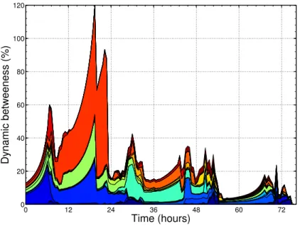
3.3 Evolution of dynamic betweeness centrality of nodes in Infocom05 trace . . 34
3.4 Impact of node 34 on the shortest dynamic paths from and to the other nodes at t = 22h (Infocom05 trace) . . . 35
3.5 Shortest dynamic paths from node 31 at t = 22h in Infocom05 trace, before (in red) and after (in blue) removal of node 34 . . . 35
3.6 Small-world network configuration. . . 37
3.7 Small-world phenomenon in dynamic networks . . . 37
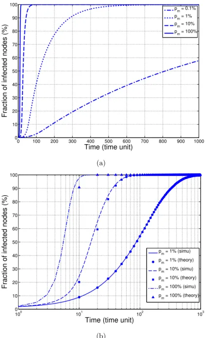
3.8 (a) Evolution of fraction of infected nodes over time (theory). (b) Com-parison of analytical and simulation results . . . 38
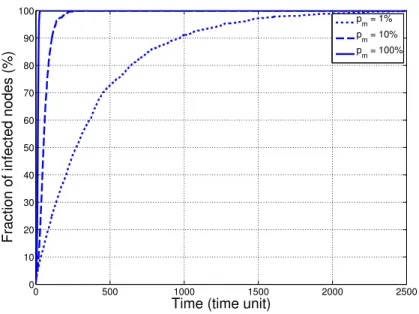
3.9 Evolution of fraction of infected nodes over time with the complete version of the model (simulation result) . . . 39
4.1 Time structure of a DTN . . . 49
4.3 Performance comparison of all algorithms . . . 55
4.4 Delivery delay of GRAD-DOWN with a network of 20, 50 or 100 nodes . . 57
4.5 Contacts map (from the top, p = 0, 0.1, 0.2, 0.5, 1 respectively) . . . 58
4.6 Shortcuts introduced by disorder reduces message passing path length . . . 58
4.7 Message passing chains (from the top, p = 0, 0.1, 0.2, 0.5, 1 respectively) . . 59
4.8 Average message passing chain length . . . 60
4.9 Building block of the Markov chain modeling the message passing process . 61 4.10 Average delivery delay of FIRST-CONTACT in function of rewiring rate for 100-nodes networks (theoretical result) . . . 63
4.11 Average delivery delay of GRAD-DOWN algorithm in function of rewiring rate for 100-nodes networks (theoretical result). . . 64
5.1 Evolution over time of the average shortest path length of real DTNs . . . 70
5.2 Symmetry of the shortest paths in Infocom05 trace . . . 71
5.3 The involvement of a node on the shortest path of another node is inversely proportional to the average inter-contact time between these two nodes . . 72
5.4 Example of the interest dissemination phase . . . 75
5.5 Correlation between the utility values of a node and the shortest dynamic path length from that node to the content subscriber . . . 77
5.6 Delivery delay of SIR vs optimal solution . . . 77
5.7 Initial spatial distribution of nodes in STEPS simulations . . . 78
5.8 Scenario A - Routing performances of the three routing protocols under different mobility contexts . . . 80
5.9 Scenario B - Routing performances comparison of the three routing proto-cols under different connectivity levels . . . 81
5.10 Scenario C - Scalability of the three routing protocols . . . 82
6.1 Typical static neighborhood topologies vs dynamic neighborhood topology generated by the mobility model . . . 90
6.2 Impact of mobility on the convergence delay of PSO algorithm . . . 92
6.3 Node spatial distribution . . . 93
6.4 Mobile cloud computing in small-world networks . . . 94
6.5 Resilience of mobile cloud network distributed services under various mo-bility contexts . . . 95
2.1 Infocom 2006 trace . . . 19
2.2 Node categories for the contact-time measure. . . 19
3.1 Dataset of real opportunistic network traces . . . 32
4.1 Estimated disorder degree of real dynamic networks . . . 52
4.2 Probabilities of contacts during the rewiring cycle . . . 60
5.1 Vector of correlation coefficients for all nodes (Infocom05 dataset) . . . 76
5.2 Simulation Configurations . . . 79
5.3 Scenario C settings . . . 82
Introduction
Contents
1.1 Dynamic networks . . . 1
1.2 Modeling Dynamic Networks . . . 2
1.3 Behavioral and Structural Properties of Dynamic Networks . 3
1.4 Routing in Dynamic Networks . . . 4
1.5 Organization of this thesis . . . 6
1.1
Dynamic networks
Nowadays, we are living in the world of mobile technologies. The two past decades witnessed the sky-rocketing development of mobile telephony. From 12 millions in 1990, the number of worldwide mobile phone subscribers hits 6 billions by the end of 2011, an impressive figure in a world of 7 billions people. With the advent of tablets, PDAs, laptops, the utility of these handheld devices are now not limited to telephoning only, instead users also use them to access to the Internet anywhere at anytime. This ubiquitous world of mobile and wireless systems has important impacts not only on everyday life of people by gradually changing their habits of communication but also at the economic, industrial and cultural levels with lots of new forms of applications, services and usages.
In such mobile space, the last recent years were the golden years of mobile applications which conducted to a dramatic growth of mobile data traffic over the Internet, specifically mobile video. In 2011, mobile data traffic was 8 times the size of the entire global Internet in 2000. And it is expected that this amount of data will still increase at high pace in the near future. This stresses the importance for research and development on higher
performance mobile networks. The great majority of mobile network services are actually operated in infrastructure mode provided by Internet Service Providers. Specifically, users can access to services either through Wi-Fi hotspots or cellular network. This poses the problem of disconnection in zones where there is no such infrastructure-based networks. One way to solve this problem is using ad-hoc communication. Mobile Ad-hoc and Delay/Disruption Tolerant Networks fall in this type of network and are still the focus of research and experiments. In these networks, dynamic nodes no longer rely on the infrastructure to communicate but use the store-move-and-forward communication paradigm to deliver information, usually via opportunistic contacts. By freeing user from the infrastructure dependence, these dynamic networks offers potentially free pervasive services which complement the existing infrastructure-based network services. Research envisions the use of spontaneous networks in workspaces, entertainment center, battle field communication, disaster recovery networks, deep space communication among planets, vehicular ad-hoc communication, etc.
Although the concept is promising and seductive, it raises several challenges to both theoretical and experimental network science. The dynamic nature of the network makes classical approaches applied for infrastructure-based networks impracticable. Classical protocols basically based on the assumption of an end-to-end path cannot be applied due to the lack of guarantee for such path in this dynamic context. Consequently, there is the need for a deep understanding of the nature of these networks and for proposing adapted communication solutions. One of the most basic and interesting open questions is how to deliver efficiently messages between dynamic nodes. This thesis aims to answer this question by first proceeding to an in-depth analysis on the nature of dynamic networks and then providing an efficient practicable routing solution based on the intrinsic properties of these networks.
1.2
Modeling Dynamic Networks
Dynamic networks, as defined in the previous paragraph, are formed by human op-portunistic contacts and hence are strongly tied to human dynamics expressed through the movements. As the first step to understand the nature of these networks, we provide a model to capture various characteristics of human mobility usually observed in real traces. It was shown that human movement has preferential attachment and attraction to geographic zones properties. This means that people moves often between a few sites
and have a high probability to return to these sites. It was also shown that the flight distance of human movement follows a power law.
Traditionally, mobile networking researches are based on simple mobility models, e.g. Random Waypoint, Random Direction models, in which parameters are chosen from an uniform distribution. These models are simple and mathematically tractable but not realistic. They fail to express the basic characteristics of human mobility and hence intro-duce biases to research results in dynamic networks. Therefore a more realistic and still tractable model is necessary for mobile networking community. Some elaborated mobil-ity models are proposed but they are either too complex for analysis or miss important features such as reflect network protocol performance as observed in real situation.
In this thesis, we provide a mobility model that captures a large spectrum of human mobility features, reflect with high fidelity salient characteristics of human movement,
and still is simple to implement and mathematically tractable [1]. This first contribution
serves as a foundational brick for the next part of the thesis.
1.3
Behavioral and Structural Properties of Dynamic
Networks
Based on the previously introduced model, we study the spatio-temporal structure of dynamic networks. The research about dynamic networks under the umbrella of network science is still new and then there is still a few insight about how these networks evolve at the spatio-temporal structural level. The understanding of these characteristics of dynamic networks, like for the static networks’ counterparts, are necessary for designing and implementing efficient network protocols, especially for solving the routing problem that we address in this thesis.
In the context of static networks, it was observed the emergence of small-world struc-ture in which the clustering coefficient is high and the shortest path length is short. This special structure allows information to spread as fast as in a random network. Many real static networks exhibit these properties. In this thesis, by extending the notion of clustering and shortest path to spatio-temporal domain, we show that dynamic networks have similar behaviors. Moreover, we show that highly mobile nodes are one of the factors
contributing to the emergence of the small-world phenomenon in dynamic networks [2].
On the other hand, we investigate contact patterns in dynamic networks. It was shown that human contacts exhibit some degree of regularity and periodicity. We propose a
model to capture this contact regularity and order degree in dynamic networks and show that, if correctly exploited, the disorder can improve significantly information routing
in such networks [3, 4]. We propose two routing algorithms that exploit the temporal
structure of human contact network to route information with a good tradeoff between resources and performance. These findings are the theoretical foundations of our routing solution.
1.4
Routing in Dynamic Networks
Basically, routing is the process of selecting a path to send messages from a sender to a receiver. This is the core process of any communication systems. For instance, the postal service performs this process to find the fastest way to send parcels while minimizing the operational cost; in the old time, telephone network operators switched jacks to make connections between two telephones. Network operators employ routing protocols to route data packets between autonomous systems, etc. In the Internet, routing algorithms are implemented in each router to assure this process. When a packet arrives at a router, the algorithm is in charge of selecting the next destination to forward the package.
Nowadays, the Internet functions based on the Internet Protocol (IP). IP is the prin-cipal protocol assuring the packet routing between hosts in the Internet. Traditionally, routers use IP address which is a binary suites assigned for each network interface to forward datagrams over the network. IP address is the analog of postal address. Each host has an IP table which consists of addresses of known hosts. When a sender host has a packet to send to a destination host, it writes its IP address and the destination’s address in the IP packet header before sending the packet to another host. The routers when receiving the packet check the IP address of the destination, consult their IP table and then use the routing algorithm to find the next host to forward the package. This process occurs at different level of the Internet (i.e., local, intra domain, inter domain) depending on the position of the source and the destination. The routing algorithm may be different at each level.
In an infrastructured environment, routing algorithms are based on the assumption that an end-to-end path between the sources and the destination exists. On the contrary in a dynamic network, nodes and links are unstable, making that end-to-end paths are not guaranteed. For instance, a node can be disconnected from the network because it is out of radio range of other nodes or because of battery shortage. Basically, routing in
such environment must rely on the store-move-and-forward communication mechanism in which relay nodes keep messages in their buffer until the next opportunistic contact with another node.
Besides, with the huge amount of content, content sharing becomes one of the most important usage of the Internet. Unfortunately, the Internet was invented with the host-centric idea in mind (i.e. to make communication between two host) and hence tie the content identity with IP address of the host storing the content. This tight coupling is not suitable for the new usage of the Internet of today. For instance, it poses problem by forcing users to rely on an address resolution system to retrieve a content which might be stored in many servers over the Internet. The new content-centric communication paradigm aims to solve these problems by considering the content as the first class citizen in the Internet world. Specifically, in such paradigm, IP address is replaced by content name. Routing in a content-centric manner means that using the content name to request and retrieve the content. This is usually based on the publish-subscribe mechanism in which users subscribe for a content and the content providers publishes and send the requested content to the users.
Applying the content-centric paradigm in the context of dynamic networks is the most suitable manner to enable content sharing over dynamic environment. Using IP and the implementation of an address resolution is inefficient due to the continuously changing topology of dynamic networks. The main problem is how to choose the relay nodes that minimize some cost functions, e.g., delay or delivery ratio, in such dynamic environment. This is a hard problem because nodes have generally only a local view of the network. Basically, researches propose heuristics which can be divided in two categories: oblivious and non-oblivious routing approaches. In the first approach, routers forward packets to any encountered node without considering the network context. The second approach consists of using local informations learned through opportunistic contacts, e.g., contact history or social information, to select good relays.
In this thesis, leveraging on the theoretical findings previously studied, we propose an
efficient routing protocol for content-centric dynamic networks [5, 6,7]. In this protocol,
nodes maintain an utility function that sums up their proximity to the destination and update the utility value at each opportunistic contact. The utility values form a gradient field in the network allowing contents to “flow” along the steepest slopes to reach the destinations. We show that this protocol outperforms classical approaches.
1.5
Organization of this thesis
The main contributions of this thesis are structured as follows. In Chapter 2, we
propose STEPS – a simple parametric model which covers a large spectrum of human mobility patterns. The model implements two seminal features of human mobility, i.e., preferential attachment and attractors. We show that this model can capture various char-acteristics of human mobility usually observed in real traces, e.g., inter-contact/contact time distribution.
In Chapter 3, we study dynamic networks in both space and time domain to extract
their salient structural characteristics. Specifically, we show that highly dynamic nodes can play the role of bridge between disconnected components and help to reduce signifi-cantly the characteristic path length of the network, hence contributing to the emergence of the small-world structure in dynamic networks. In STEPS, starting from a regular dynamic network in which nodes tend to stay in their preferential zones, we rewire it by progressively increasing the percentage of nomadic nodes in the network. We show that, as soon as the ratio of nomadic nodes passes 10%, the network exhibits a small-world properties with a high dynamic clustering coefficient and a low shortest dynamic path length.
In chapter 4, we study temporal contact patterns in dynamic networks, on
particu-lar their disorder degree. We show that real dynamic networks exhibits some degree of disorder and irregularity which, if correctly exploited, improves significantly routing per-formances. First, we introduce a model for the disorder degree of dynamic networks. This model allows us to rewire contacts in a totally regular temporal network with a probabil-ity p, so injecting some disorder degree into the network. We then investigate intensively real dynamic network and found that their disorder degree ranges from medium to high
(preal ranges from 50% to 70%). We introduce a simple but efficient greedy algorithm
which leverages on the temporal structure of dynamic networks to deliver messages with a good performance/resource tradeoff. Simulation and analytical analysis show that this algorithm outperforms other approaches. Moreover, the algorithm achieves its optimal performance in networks with a disorder degree of 20%.
Based on the idea developed in Chapter 4, in Chapter 5, we propose a new efficient
routing protocol for content-centric dynamic network. In this protocol, nodes maintain an utility function which summarizes their spatio-temporal proximity to the destination node. The utility values update is performed during each opportunistic contact. Consequently, a gradient field is formed in the network allowing the messages to flow along the steepest
slope to reach the destination. This routing algorithm can be easily adapted to both address-centric or content-centric dynamic networks. Simulation results show that the protocol outperforms classical routing protocols for DTNs.
Chapter 6 brings out a potential application of content-centric dynamic networks in
the context of mobile cloud computing. In this chapter, by applying swarm optimization techniques, we show that mobility can increase dramatically the processing capacity of dynamic networks. On the other hand, we show that the network structure has also an
important impact on the processing capacity of the network [8].
Understanding and Modeling Dynamic
Networks
Contents
2.1 Introduction . . . 10
2.2 Related works . . . 10
2.3 Characterizing & Modeling Human Mobility . . . 12
2.3.1 STEPS . . . 13
2.3.2 The Underlying Markov Chain . . . 14
2.4 Fundamental Properties of Opportunistic Networks in STEPS 17
2.4.1 Inter-Contact Time Distribution . . . 17
2.4.2 Contact Time Distribution . . . 19
2.4.3 Routing Performance . . . 20
2.4.4 Understanding Opportunistic Network Structure with STEPS . 21
2.5 Conclusion. . . 23
Mobility is the seminal process which underlines dynamic networks composed of human portable devices. In this chapter, we are interested in the modeling of such dynamic net-works. We introduce Spatio-TEmporal Parametric Stepping (STEPS) – a simple paramet-ric mobility model which can cover a large spectrum of human mobility patterns. STEPS abstracts spatio-temporal preferences in human mobility by using a power law to rule the nodes movement coupled with two fundamental mobility principles. Nodes in STEPS have preferential attachment to favorite locations where they spend most of their time. Via simulations, we show that STEPS is able, not only to express peer to peer properties such as inter-contact/contact time and to reflect accurately realistic routing performance, but
also to express the structural properties of the underlying interaction graph such as the small-world phenomenon. Moreover, STEPS is easy to implement, flexible to configure and also theoretically tractable.
2.1
Introduction
Human mobility is known to have a significant impact on performance of opportunistic networks. Unfortunately, there is no model that is able to capture all the characteristics of human mobility due to its high complexity. We introduce Spatio-TEmporal Parametric Stepping (STEPS) – a powerful formal model for human mobility or mobility inside social/interaction networks. The introduction of this new model is justified by the lack of modeling and expressive power, in the currently used models, for the spatio-temporal correlation usually observed in human mobility.
We show that preferential location attachment and location attractors are invariants properties, at the origin of the spatio-temporal correlation of mobility. Indeed, as observed in several real mobility traces, while few people have a highly nomadic mobility behavior the majority has a more sedentary one.
We assess the expressive and modeling power of STEPS by showing that this model successes in expressing easily several fundamental human mobility properties observed in real traces of dynamic network:
– The distribution of human traveled distance follows a truncated power law. – The distribution of pause time between travels follows a truncated power law. – The distribution of inter-contact/contact time follow a truncated power law. – The underlying dynamic graph can emerge a small-world structure.
The rest of this chapter is structured as follows. After an overview of the state of the
art in Section2.2, we present the major idea and formally introduce STEPS in Section2.3.
Section 2.4 shows the capacity of STEPS to capture salient features observed in real
dy-namic networks, going from inter-contact/contact time to epidemic routing performances
and small-world phenomenon. Finally we conclude the chapter in Section2.5.
2.2
Related works
Human mobility has attracted a lot of attention of not only computer scientists but also epidemiologists, physicists, etc because its deep understanding may lead to many
other important issues in different fields. The lack of large scale real mobility traces made that research is initially based on simple abstract models, e.g., Random Waypoint,
Random Walk (see [9] for a survey). These models whose parameters are usually drawn
from an uniform distribution, although are good for simulation, can not reflect the reality
and even are considered counterproductive in some cases [10]. In these models, there is
no notion of spatio-temporal preferences.
Recently, available real data allowed researchers to understand deeper the nature of human mobility. The power law distribution of the traveled distance was initially reported
in [11] in which the authors study the spatial distribution of human movement based on
bank note traces. The power law distribution of the inter-contact time was initially studied
by Chaintreau et al. in [12]. In [13], Karagiannis et al. confirm this and also suggest that
the inter-contact time follows a power law up to a characteristic time (about 12 hours) and then cut-off by an exponential decay.
In [14], the authors show that people have a significant probability to return to a
few highly frequented locations. Another study [15] shows that humans show significant
propensity to return to the locations they visited frequently before, like home or workplace. These two intrinsic human mobility characteristics, i.e., location preference and attractor, are implemented in our model.
Some more sophisticated mobility models have been proposed. In [16], the authors
have proposed an universal model being able to capture many characteristics of human daily mobility by combining different sub-models. With a lot of parameters to configure, the complexity of this type of model makes them hard to use.
In [17], the authors propose SLAW – a Random Direction like model – except that the
traveled distance and the pause time distributions are ruled by a power law. An algorithm for trajectory planning was added to mimic the human behavior for always choosing the optimal path. Although being able to capture statistical characteristics like inter-contact, contact time distribution, the notion of spatio-temporal preferential attachment is not covered by this model.
Another modeling stream aims to integrate social behaviors. In [18], a community
based model was proposed in which the movement depends on the relationship between nodes. The network area is divided in zones and the social attractivity of a zone is based on the number of friends in the same zone. The comparisons of this model with real traces show a difference for the contact time distribution.
model the location preference and periodical re-appearance of human mobility by creating community zones. Nodes have different probabilities to jump in different communities to capture the location preference. Time structure was build on the basis of night/day and days in a week to capture the periodical re-appearance. However, fundamental features of human trajectories such as traveled distance distribution and inter-contact/contact time distributions were not highlighted.
Recent research shows that some mobility model (including [19]), despite of their
capacity of capturing spatio-temporal characteristics, deviate significantly in routing
per-formances when compared to the ones obtained with real traces [20]. This aspect that
has not always been considered in existing models is indeed really important because it shows the capacity of a model to reproduce a fundamental feature of a dynamic network.
2.3
Characterizing & Modeling Human Mobility
STEPS is inspired by observable characteristics of the human mobility behavior, specifically the spatio-temporal correlation. Indeed, people share their daily time be-tween some specific locations at some specific time, e.g., home/office, night/day. These spatio-temporal patterns repeat at different scales and has been recently observed on real
traces [19].
On a short time basis, i.e., a day, a week, we can assume that one have a finite space of locations. According to these observations, we define two mobility principles:
• Preferential attachment: the probability for a node to move in a location is inversely proportional to the distance from his preferential location.
• Attractor: when a node is outside of his preferential location, he has a higher probability to move closer to this location than moving farther.
From this point of view, the human mobility can be modeled as a finite state space Markov chain in which the transition probability distribution expresses a movement
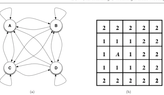
pat-tern. Figure2.1(a)illustrates a Markov chain with 4 states which correspond to 4 locations
of interest.
In STEPS, a location is modeled as a zone which corresponds to a Markov chain state. Inside a zone, nodes can move freely according to a random mobility model such as Ran-dom Waypoint. The displacement between zones is drawn from a power law distribution whose the exponent value expresses the more or less nomadic behavior. By simply tuning the power law exponent, STEPS can cover a large spectrum of mobility patterns from
(a) (b)
Figure 2.1: (a) Human mobility modeling under a markovian view: States represent different localities, e.g., House, Office, Shop and Other places, and transitions represent the mobility pattern. (b) 5 × 5 torus representing the distances from location A to the other locations.
purely random ones to highly localized ones. Besides, complex heterogeneous mobility behavior can be described by combining nodes with different mobility patterns as de-fined by their preferential zones and the related attraction power. Group mobility is also supported on our implementation. Hereafter, we give the details of this model.
2.3.1
STEPS
Assume that the network area is a square torus1 divided in N square zones. The
distance between zones is defined according to a metric. We use Chebyshev distance in
this case. Figure2.1(b)illustrates an example of a 5 × 5 torus with the distances from the
zone A. One can imagine a zone as a geographic location (e.g., home, school, supermarket) or a logical location (i.e., a topic of interest such as football, music, philosophy, etc). Therefore, we can use the model to study both human geographic mobility and human social behaviors. In this thesis, we deal only with the first case.
In such structured space, each mobile node is associated with a preferential zone zpref.
For the sake of simplicity, we assume that each node is attached to one zone. However, this 1. The choice of a torus allows to have a homogeneous area.
model can be extended by associating a node with several preferential zones. The node movement between zones is driven by a power law satisfying the two mobility principles described above. The probability mass function of this power law is given by
P [D = d] = β
(1 + d)α, (2.1)
where D is a discrete random variable representing the distance from zpref, α is the power
law exponent that represents the attraction power of zprefand β is a normalizing constant.
From Equation 2.1 we can see that, the farther a zone is from the preferential zone,
the less probability the node to move in. This is the principle of preferential attachment. On the other hand, when a node is outside its preferred zone, it has a higher probability to move closer to this one than moving farther. This is the principle of attraction. In consequence, with a power law, the model is able to capture two basic characteristics of human mobility.
This small set of modeling parameters allows the model to cover the full spectrum of mobility behaviors. Indeed, according to the value of the α exponent a node can have a more or less nomadic behavior. For instance,
– when α < 0, nodes have a higher probability to choose a long distance than a short one and so the preferential zone plays a repulsion role instead of a attraction one; – when α > 0, nodes are more localized, hence tend to stay in their preferential zones; – when α = 0, nodes move randomly towards any zone with a uniform probability.
We summarize the details of STEPS in Algorithm 1. A MATLAB implementation of
STEPS can be downloaded at [21].
2.3.2
The Underlying Markov Chain
In this section, we give the details and the properties of the Markovian model under-lying STEPS. Wherever node’s preferential zones are, the torus structure gives different nodes the same spatial structure, i.e., they have the same number of zones with a given distance from their preferential zones. More specifically, for a distance d, we have 8d zones
with equal distances from zpref. Consequently, the probability for a node to choose one
among these zones is
P!zi, dzizpref = d" = 1
8dP [D = d] =
β
8d(1 + d)α. (2.2)
Because the probability for a node to select a destination zone zi depends only on the
Input: Initial zone ← zpref
1 repeat
2 Choose a random distance d from the probability distribution (2.1);
3 Select uniformly at random a zone zi among all zones that are d distance units
away from zpref;
4 Choose uniformly at random a point in zi;
5 Go linearly to this point with a speed chosen uniformly at random from
[vmin, vmax] , 0 < vmin ≤ vmax< +∞;
6 Choose uniformly at random a staying time t from
[tmin, tmax] , 0 ≤ tmin ≤ tmax < +∞;
7 while t has not elapsed do
8 Perform Random Waypoint movement in zi;
9 end
10 until End of simulation;
Algorithm 1: STEPS algorithm for a node
to select zi. If we define the transition probabilities of the Markov chain as a
stochas-tic matrix, this one will have idenstochas-tical rows. The matrix is then idempotent, i.e., the multiplication by itself gives the same matrix. This matrix is given by
P (z0) P (z1) . . . P (zN−1) ... ... . .. ... P (z0) P (z1) . . . P (zN−1) . (2.3)
It is straightforward to deduce the stationary state of the Markov chain which is
Π =)P (z0) P (z1) . . . P (zN−1)
*
. (2.4)
From this result, it is interesting to characterize the inter-contact time2 of STEPS
because this network property was shown to have important impacts on forwarding al-gorithm in opportunistic networks. To simplify the problem, let assume that a contact occurs if and only if two nodes are in the same zone and node’s movement is limited to jumping between zones. Let two nodes A and B move according to the STEPS model, starting initially from the same zone. The probability that the two nodes are in the same
zone at a given time is pcontact= PA(z0)PB(z0) + . . . + PA(zn−1)PB(zn−1) = N−1 + i=0 P (zi)2 = dmax + d=0 1 8d , β (d + 1)α -2 , (2.5) where dmax= % √ N
2 & is the maximum distance between zones in the torus.
Let ICT be the discrete random variable which represents the time elapsed before A and B are in contact again. One can consider that ICT is the number of trials until the
first success of an event with probability of success pcontact. Hence ICT follows a geometric
distribution with the parameter pcontact. Therefore, the probability mass function of ICT
is given by
P [ICT = t] = (1 − pcontact)t−1pcontact. (2.6)
It is well known that the continuous analog of a geometric distribution is an expo-nential distribution. Therefore, the inter-contact time distribution for i.i.d. nodes can be approximated by an exponential distribution. This is true when the attractor power α is equals to 0, i.e., when nodes move uniformly, because there is no spatio-temporal corre-lation between nodes. But when α (= 0, there is a higher correcorre-lation in their movement and in consequence the exponential distribution is not a good approximation. Indeed,
in [22], the authors report this feature for the Correlated Random Walk model where
the correlation of nodes induces the emergence of a power law in the inter-contact time distribution. In the following, we provide simulation results related to this feature for STEPS.
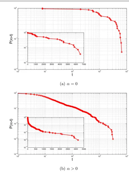
Figure 2.2 gives the log-log and linear-log plots of the complementary cumulative
distribution function or CCDF of the inter-contact time that results from a simulation of the Markov chain described above when α = 0 and α > 0. In the first case, the inter-contact time distribution fits an exponential distribution (i.e., is represented by a linear function in the linear-log plot) while in the second case it fits a power law distribution (i.e., is represented by a linear function in the log-log plot) with an exponential decay tail. These results confirm the relationship between the spatio-temporal correlation of nodes and the emergence of a power law in inter-contact time distribution.
(a) α = 0
(b) α > 0
Figure 2.2: Theoretical inter-contact time distribution of STEPS
2.4
Fundamental Properties of Opportunistic Networks
in STEPS
It is worth mentioning that a mobility model should express the fundamental properties observed in real opportunistic networks. In this section, we show that STEPS can, indeed, capture the salient characteristics of human mobility.
2.4.1
Inter-Contact Time Distribution
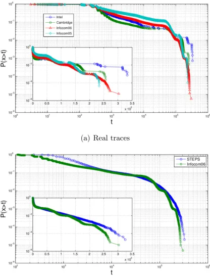
The inter-contact time is defined as the delay between two encounters of a pair of nodes. Real traces analysis suggest that the distribution of inter-contact time can be approximated by a power law up to a characteristic time (i.e., about 12 hours) followed
by an exponential decay [13]. In the following we will use the set of traces presented
by Chaintreau et al. in [12] as base of comparison with STEPS mobility simulations.
Figure 2.3(a) shows the aggregate CCDF of the inter-contact time3 for different traces.
In order to demonstrate the capacity of STEPS to reproduce this feature, we configured STEPS to exhibit the results observed in the Infocom 2006 conference trace which is the
largest trace in the dataset. Table 2.1 summarizes the characteristics of this trace.
(a) Real traces
(b) STEPS vs Infocom06 trace
Figure 2.3: CCDF of Inter-Contact Time
To simulate the conference environment, we create a 10 × 10 torus of size 120 × 120m2
that mimics rooms in the conference. The radio range is set to 10m which corresponds to Bluetooth technology. The node speed is chosen as human walking speed which ranges
from [3, 5] km/h. Figure 2.3(b) shows the CCDF of the resulting inter-contact time in
Characteristic Value
Number of nodes 98
Duration 4 days
Connectivity Bluetooth
Average inter-contact time 1.9 hours
Average contact duration 6 minutes
Table 2.1: Infocom 2006 trace
Mobility degree RWP pause time range (s) Number of nodes
Very high [0, 60] 65
High [60, 900] 15
Low [900, 3600] 10
Very low [3600, 43200] 8
Table 2.2: Node categories for the contact-time measure
log-log and lin-log plots. We observe that the resulting inter-contact time distribution given by the STEPS simulations fits with the one given by the real trace.
2.4.2
Contact Time Distribution
Because of the potential diversity of nodes behaviors, it is more complicated to repro-duce the contact duration given by real traces. Indeed, the average time spent for each contact depends on the person. For instance, some people spend a lot of time to talk while the others just check hands. We measured the average contact duration and the average node degree, i.e., the global number of neighbor nodes, of the Infocom06 nodes and ranked them according to their average contact duration. The result is reported in
Figure2.4(a). According to this classification, it appears that the more (resp. less)
popu-lar the person is, the less (resp. more) time he or she spends for each contact. Because the contact duration of STEPS depends principally on the pause time of the movement inside zone (i.e., the pause time of RWP movement), to mimic this behavior with STEPS, we divided nodes in four groups. Each group corresponds to a category of mobility behavior: highly mobile, mobile, slightly mobile and rarely mobile. The pause time for each groups
is summarized in Table 2.2.
trace where a large percentage of nodes have short contacts and a few nodes have long to very long contacts. The CCDFs of contact time of STEPS and Infocom06 trace as shown
in Figure 2.4(b) show that STEPS can also capture with a good accuracy this mobility
behavior.
(a) Social characteristic observed in Infocom06 trace
(b) CCDF of contact time of STEPS vs Infocom06 trace Figure 2.4: Contact time behavior of STEPS vs real trace
2.4.3
Routing Performance
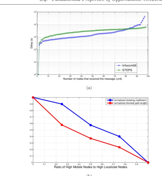
An often neglected feature when introducing a mobility model is its ability to reproduce the performances given by routing protocols on top of real traces. In order to assess the capacity of STEPS to offer this important property, we ran Epidemic routing on STEPS and Infocom06 trace and compared the respective routing delays. For each trace, the average delay to spread a message is measured as a function of the number of nodes who
(a)
(b)
Figure 2.5: (a) Epidemic routing delay of STEPS vs Infocom06 trace. (b) Small-world structure in STEPS
received the message. Figure2.5(a)shows that STEPS is able to reflect at the simulation
level the performance of Epidemic routing when applied on real traces.
2.4.4
Understanding Opportunistic Network Structure with STEPS
A good mobility model should allow not only to express faithfully peer-to-peer in-teraction properties such as inter-contact time and contact time, but also to reproduce the fundamental structure of the underlying interaction graph as modeled by a temporal graph, i.e. graphs with time varying edges. The structural properties of static interaction graphs have been studied leading to the observation of numerous instances of real
of graph is called small-world. With respect to routing, the small world structure induces fast message spreading in the underlying network.
Our research on the small-world phenomenon in dynamic networks is fully detailed in
Chapter3. In this chapter, we provide only the preliminary ideas which lead to those final
results. Specifically, this is our first attempt to extend the notions of clustering coefficient
and shortest path length introduced in [23] for dynamic networks.
Let G(t) = (V(t), E(t)) be a temporal graph with the time varying set of vertexes V(t) and the time varying set of edges E(t). We define the temporal clustering coefficient and temporal shortest path length as follows.
– Temporal clustering coefficient : Let N (w, i) be the set of neighbors of node i for a time window w. The temporal clustering coefficient is defined as the ratio of the actual number of connections between the neighbors of i to the possible number of connections between them during the time window w. Intuitively, it represents the cliquishness of a time varying friendship circle. Formally, that is
Ci =
2.
j|N (w, j) ∩ N (w, i)|
|N (w, i)| (|N (w, i)| − 1), (2.7)
where j is a neighbor of i and |X| denotes the cardinal of X.
– Temporal shortest path length : Let Rij(t) ∈ {0, 1} denotes a direct or indirect
connection, i.e., via multiple connections at different times, between node i and node j at time t. The shortest path length between i and j is defined as the earliest
time from an initial time t0 when there is a connection between them. That is
Lij = inf{t|Rij(t) = 1}. (2.8)
To visualize the phenomenon in STEPS, we create scenarios where there are two categories of nodes with different attraction power. In the first category, nodes have a high mobile behavior (i.e., α is small) while in the second one, they are more localized (i.e., α is large). The idea is to “rewire” a highly clustered and weakly dynamic network (i.e., with the population in the second category) by introducing highly mobile nodes into that graph. By tuning the ratio of number of nodes between these two categories,
we measure the metrics defined in (2.7) and (2.8). Figure 2.5(b) shows that between
a regular and random structure, the network exhibits structures where the temporal clustering coefficient is high while the temporal shortest path length is low. This first result suggests the existence of the small-world phenomenon in dynamic graphs which
will be studied in Chapter 3. Moreover, this result shows the expressive capacity of
2.5
Conclusion
In this chapter, we have introduced STEPS, a generic and simple mobility model which abstracts the spatio-temporal correlation of human mobility. Based on the principles of preferential attachment and location attractor, this model can cover a large spectrum of human mobility patterns by tuning only a small set of parameters. Via simulations, the model is shown to be able to capture different characteristics observed within real mobility traces. Moreover, the model can also reflect accurately realistic routing performances, one of important aspect often neglected in proposed mobility models. In addition, STEPS can also capture the structural properties of the underlying dynamic graph. Finally, the underlying Markovian basis make it possible to derive analytical results from the model. This model plays the role of a foundational brick for our subsequent researches throughout this thesis.
Small-World Structure of Dynamic
Networks
Contents
3.1 Introduction . . . 26
3.2 Related works . . . 27
3.3 Small-world Phenomenon in Dynamic Networks . . . 28
3.3.1 Dynamic Small-world Metrics . . . 28
3.3.2 Opportunistic Network Traces Analysis . . . 31
3.4 Modeling Dynamic Small-world Structure with STEPS . . . 36
3.5 Information diffusion in Dynamic Small-world Networks . . . 38
3.6 Conclusion. . . 41
The small-world phenomenon first introduced in the context of static graphs consists of graphs with high clustering coefficient and low shortest path length. This is an intrinsic property of many real complex static networks. Recent research has shown that this struc-ture is also observable in dynamic networks but how it emerges remains an open problem. In this chapter, we first formalize the metrics to qualify the small-world structure and then investigate in-depth various real traces to highlight the phenomenon. With help of STEPS, we point out that highly mobile nodes are at the origin of the emergence of the small-world structure in dynamic networks. Finally, we study information diffusion in such small-world networks. Analytical and simulation results with epidemic model show that the small-world structure increases significantly the information spreading speed in dynamic networks.
3.1
Introduction
In his famous experiment, Milgram showed that the human acquaintance network has a diameter in the order of six, leading to the small-world qualification. Watts and Strogatz
later introduced a model of small-world phenomenon for static graphs [23]. They proposed
a random rewiring procedure for interpolating between a regular ring lattice and a random graph. Between these two extrema, the graph exhibits an exponential decay of the average shortest path length contrasting with a slow decay of the average clustering coefficient. Interestingly, numerous real static networks exhibit such property. From a communication perspective, Watts and Strogatz also pointed out that a small-world network behaves as random network in terms of information diffusion capacity.
However, the great majority of studies on small-world networks properties and be-haviors focused on static graphs and ignored the dynamics of real mobile networks. For example, in a static graph, an epidemic cannot break out if the initial infected node is in a disconnected component of the network; conversely in a mobile network, nodes move-ments can ensure the temporal connectivity of the underlying dynamic graph. Moreover, an epidemic can take off or die out depending not only on the network structure and the initial carrier, but also on the time when the disease begins to spread. These aspects cannot be captured by a static small-world model.
In order to formalize the dynamic small-world phenomenon, we extend to dynamics networks the notions of dynamic clustering coefficient and shortest dynamic path. By studying the evolution of these metrics from our rewiring process, we show the emergence of a class of dynamic small-world networks with high dynamic clustering coefficients and low shortest dynamic path length. We then demonstrate the capacity of STEPS to capture these structural characteristics of mobile opportunistic networks by showing that, when increasing progressively the dynamicity of a network from an initial stable state, then this rewiring process entails the emergence of a small-world structure.
The rest of the chapter is structured as follows. Section 3.2 introduces previous works
that inspired our contribution. In Section3.3, after having formally defined the notions of
dynamic clustering coefficient and shortest dynamic path length, we analyze various real traces and show the intrinsic properties of dynamic networks that induce the small-world phenomenon. We show how the small-world structure emerge in dynamic networks in
Section3.4. In Section3.5, from simulations and analytical analysis, we study information
diffusion performances in dynamic small-world networks. Finally, Section 3.6 concludes
3.2
Related works
In [23], Watts and Strogatz introduce a model of small-world phenomenon in static
graphs. From a regular ring lattice, they rewire randomly edges in this graph with a probability varying from 0 (i.e. leading to a regular network) to 1 (i.e. leading a random graph). During this process they observed an abrupt decrease of the average shortest path length, leading to short path of the same order of magnitude as observed in random graphs, while the clustering coefficient is still of the same order of magnitude than the one of a regular graph. This features suggested the emergence of the small-world phenomenon. The authors also demonstrate that this graph structure, observed in many real static networks, allows information to diffuse as fast as in a random graph.
Kleinberg [24] extended the model to 2-d lattices and introduced a new rewiring
pro-cess. This time, the edges are not uniformly rewired but follow a power law 1
dα where d is
the distance on the lattice from the starting node of the edge and α is the parameter of
the model. Newman [25] proposed another definition of the clustering coefficient which
has a simple interpretation and is easier to process. The authors argue that the definition
in [23] favors vertices with low degree and introduces a bias towards networks with a
significant number of such vertices.
Although research pays much attention to the small-world phenomenon in static net-works, either through modeling or analytical analysis, the small-world phenomenon in dynamic networks like opportunistic networks is still not well understood. This is partly
due to the lack of models and metrics for dynamic graphs. Recently, J.Tang et al. [26]
defined several metrics for time varying graphs, including temporal path length, temporal clustering coefficient and temporal efficiency. They showed that these metrics are useful to capture temporal characteristics of dynamic networks that cannot be captured by tra-ditional static graph metrics. The definition of dynamic path, introduced in this paper, is close to their definition (we had the dual metric of the number of hops). We also in-troduce a new definition of dynamic clustering coefficient which captures more accurately the dynamics of opportunistic networks.
In [27], the authors highlight the existence of the small-world behavior in real dynamic
network traces. Using the definition of temporal correlation introduced in [28], they
show that real dynamic networks have a high temporal correlation and low temporal shortest path, suggesting a dynamic small-world structure. In this modeling work, we
extend consistently to dynamic networks the initial small-world metrics defined in [23]
3.3
Small-world Phenomenon in Dynamic Networks
In this section, we formalize the notion of small-world phenomenon in dynamic net-works by introducing two metrics used for qualifying such phenomenon: shortest dynamic path length and dynamic clustering coefficient. Then by analyzing extensively real op-portunistic network traces, we show fundamental characteristics which are at the origin of the dynamic small-world phenomenon.
3.3.1
Dynamic Small-world Metrics
Shortest Dynamic Path Length
Basically, the shortest path problem in static graphs consists in finding a path such that the sum of the weights of its constituent links is minimized. From a graph theory point of view a dynamic networks can be described by a temporal graph, i.e., a temporal sequence of graphs that describe the discrete evolution of the network according to nodes and links creation and destruction events. A path in a dynamic network can be seen as an ordered set of temporal links that allow a message to be transferred using the
store-move-forward paradigm between two nodes. Formally, let lt
ij be a link between node i
and node j at instant t. A dynamic path from node u to node v from time t0 to time
t is described by a time ordered set puv(t0, t) = /ltui0, l
t1
ij, . . . , ltwv0 where tk+1 > tk. We
consider two metrics of dynamic paths:
– Delay : the sum of the inter-contact times between consecutive links which consti-tutes the path.
– Number of hops : the number of temporal links which constitutes the path. This leads to the following definition of shortest dynamic path length.
Definition 1 The shortest dynamic path is the path giving the minimum amount of
delay4. If there are several paths giving the same delay, then we select the one giving the
minimum number of hops. Formally, the shortest dynamic path length between i and j
from time t0 is
Lt0
ij = inf {t − t0|∃pij(t0, t)} . (3.1)
The shortest dynamic path length of a network of N nodes from time t0 is the average of
4. we can also have another definition for minimizing the number of hops. In this work, we focus only on delay constrained path.
the shortest dynamic path lengths of all pairs of nodes in the network Lt0 = . ijL t0 ij N (N − 1) . (3.2)
To find the shortest dynamic path length of all pairs of nodes, we propose an algorithm leveraging on the following interesting property of adjacency matrix in static graphs.
The adjacency matrix A is defined as the matrix in which the element (A)i,j ∈ {0, 1}
at row i and column j denotes the existence of a link between node i and node j. If we
process the power n of such matrix, then its element (An)
i,j gives the number of paths of
length n between i and j. Indeed, for example, when n = 2, (A2)
i,j =.k(A)i,k× (A)k,j
sums all the possibilities to go from i to j through an intermediate node k. We extend
this property to dynamic networks. Let At, t = 0, 1, . . . , n be the adjacency matrix of a
dynamic network at time t. The matrix Ct obtained as follows
Ct = At∨ A2t ∨ . . . ∨ A
n
t , (3.3)
where Ai
t denotes the binary version of the matrix Ait (i.e. the element (At)i,j equals to 1
if (At)i,j > 0 and 0 otherwise) has its elements (Ct)i,j which indicate if there is a direct or
indirect link (up to n hops) between i and j at time t. Indeed, (Ct)i,j is the logical sum
of all possibilities to have a direct or indirect link (up to n hops) between i and j at time t. In consequence, the product
Dt= C0C1. . . Ct (3.4)
results in a matrix in which the element (Dt)i,j specifies, when not null, that there is
dynamic path of delay t between i and j. Therefore the shortest dynamic path length
from node i to node j is given by the smallest value of t such as (Dt)i,j equals to 1.
It is straight-forward to demonstrate that if a node k belongs to a shortest path between node i and node j then the i to k sub-path gives the shortest path between i and k. Therefore the shortest path between two nodes i and j can be easily backwardly reconstructed. Note that at time t two nodes can be connected to each other via a multiple hops path. To find the complete spatio-temporal path with all the intermediate nodes, we simply apply a breath first search each time we find a spatial multiple hops link. In practice, as it’s unlikely to have a large number of nodes connected to each other at a given moment, we can optimize the algorithm by limiting the number of iterations n in
Equation3.3 to an upper bound of the network diameter. Finally, this algorithm is more
efficient (time complexity O(n3)) than the depth first search approach as proposed in [26]
(time complexity O(n4)).
Dynamic Clustering Coefficient
As defined in [23], the clustering coefficient measures the cliquishness of a typical
friend circle. The clustering coefficient of a node is calculated as the fraction of actual existing links between its neighbors and the number of possible links between them. The clustering coefficient of a network is calculated by averaging the clustering coefficients of
all the nodes in the network. In [25], Newman defines the clustering coefficient in term of
transitivity. The connection between nodes u, v, w is said to be transitive if u connected to v and v connected to w implies that u is connected to w. The clustering coefficient of a network is then calculated as the fraction of the number of closed path of length two over the number of path of length two, where a path of length two is said to be closed if it is a transitive path. This definition is simple to interpret and easy to calculate. Considering that, the initial definition gives more weight to nodes with low degree and introduces a bias towards graph composed of several of these nodes, in this work, we favor Newman’s definition and extend it to dynamic networks.
In [26], Tang et al. first introduced a generalization of Watts and Strogatz’s definition
for temporal graph. The temporal clustering coefficient of a node during a time interval t is the fraction of existing opportunistic contacts (multiple contacts count once) between the neighbors of the node over the number of possible contacts between them during t. The clustering coefficient of the network is the average of the clustering coefficients of all the nodes. This is simply the application of Watts and Strogatz’s definition on a time snapshot of the network. While this definition was shown to better capture temporal characteristics of time varying graph, it depends strongly on the length of the chosen time interval. If this interval tends to infinity, the temporal clustering coefficient tends to 1 as all the nodes meet each other with a high probability. On the other hand, if the interval tends to 0, then conversely the temporal clustering coefficient tends to 0.
Figure 3.1 illustrates the influence of the time window size on measures of the clustering
coefficient on a real mobility trace.
In order to avoid this temporal bias, we propose a new definition of dynamic clustering coefficient which captures the dynamics of the degree of transitivity and is independent of the measuring time interval.
Definition 2 A dynamic path from node i to node j is transitive if there exists a node k
and time t1, t2, t3 so that i is connected to k at t1, k is connected to j at t2, i is connected
to j at t3 and t1 ≤ t2 ≤ t3. The dynamic clustering coefficient of node i from time t0
0 12 24 36 48 60 72 84 0 0.5 1 0 12 24 36 48 60 72 84 0 0.5 1 0 12 24 36 48 60 72 84 0 0.5 1 Time (hours) 0 12 24 36 48 60 72 84 0 0.5 1 Clustering coefficient 0 12 24 36 48 60 72 84 0 0.5 1 3 days 6 hours 3 hours 1 hours 3 minuites
Figure 3.1: Time window size effect on measure of temporal clustering coefficient (as defined in [11])
when the transitive path from i to j is formed, that is Ct0
i = t−t10. The dynamic clustering
coefficient of a network of N nodes is then calculated by averaging over the dynamic
clustering coefficient of all the nodes from time t0
C = 1
N +
i
Ci . (3.5)
We also provide a MATLAB code for computing the dynamic clustering coefficient at [30].
3.3.2
Opportunistic Network Traces Analysis
In this section, we analyze extensively real opportunistic network traces to understand how small-world behavior emerges in dynamic networks. We first apply the above defini-tions to highlight the existence of dynamic small-world phenomenon on these traces. For
that, we use the data sets from the Haggle project [12,31] which consists of the recording
of opportunistic bluetooth contacts between users in conference or office environments.
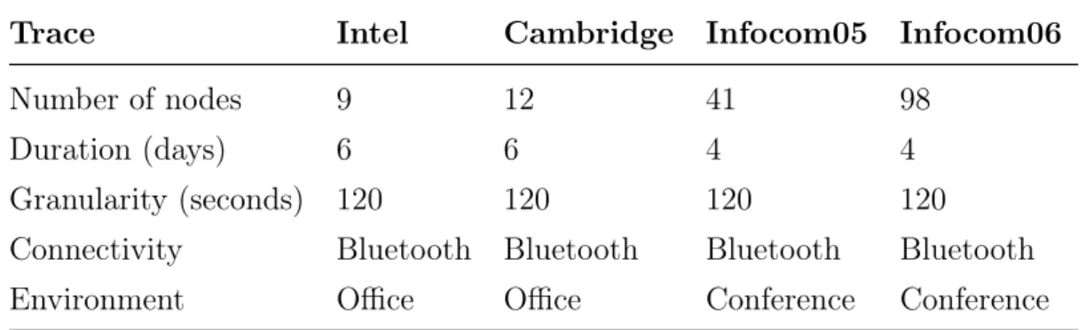
The settings of these data sets are summarized in Table3.1.
For each trace, we measure the shortest dynamic path length and the dynamic clus-tering coefficient every 2000 seconds to see the evolution of these metrics over time. The
Trace Intel Cambridge Infocom05 Infocom06
Number of nodes 9 12 41 98
Duration (days) 6 6 4 4
Granularity (seconds) 120 120 120 120
Connectivity Bluetooth Bluetooth Bluetooth Bluetooth
Environment Office Office Conference Conference
Table 3.1: Dataset of real opportunistic network traces
pattern of both metrics with a typical period of 24 hours and a phase change every 12 hours. This can be easily explained by the fact that human daily activity is periodic with nigh/day phases. Indeed, people are more nomadic during day while they are mostly sedentary at night. Besides, it is interesting to note that the dynamic clustering coeffi-cient and the shortest dynamic path length evolve in opposite phase. Despite of a slight diversity in different traces due to differences in nodes number and density, traces dura-tions, etc, during the dynamic phase (i.e., day, for instance, the period around 24 hours in Infocom2005 trace), these networks always exhibit high dynamic clustering coefficients and low shortest dynamic path lengths, suggesting the existence of a dynamic small-world phenomenon.
To explain the emergence of this phenomenon, let us focus on and analyze the structure of these networks during the dynamic phases. In the Watts and Strogatz model, the small-world phenomenon emerges when shortcut edges are randomly added to a regular graph. These shortcuts allow the average shortest path length to be reduced significantly while conserving network nodes’s cliquishness. We argue that in dynamic networks, mobile nodes are implicitly at the origin of these shortcuts. Indeed, it is known that people spend their daily life among different social communities at specific locations at different times (e.g., colleagues at office in the morning, family at home in the evening). A community can be disconnected from the others in space and/or in time. Besides, some people are more “mobile” than other, they have contacts in many communities and move often between these communities or areas. These "nomadic” nodes contribute to reduce significantly the shortest dynamic path length from nodes in a disconnected component to the rest of network and hence contribute to the emergence of the dynamic small-world phenomenon. To identify the spatio-temporal shortcuts in dynamic networks, we introduce a metric that measures the influence a node has on the characteristic dynamic path length of the
0 12 24 36 48 60 72 0 0.1 0.2 0.3 0.4 0.5 0.6 0.7 0.8 0.9 1 Time (hour) Normalized value
Dynamic clustering coefficient Dynamic shortest path distance
(a) Infocom 2005 0 12 24 36 48 60 72 84 96 0 0.1 0.2 0.3 0.4 0.5 0.6 0.7 0.8 0.9 1 Time (hour) Normalized value
Dynamic clustering coefficient Dynamic shortest path length
(b) Infocom 2006 0 12 24 36 48 60 72 84 96 108 0 0.1 0.2 0.3 0.4 0.5 0.6 0.7 0.8 0.9 1 Time (hour) Normalized value
Dynamic clustering coefficient Dynamic shortest path distance
(c) Intel 0 12 24 36 48 60 72 84 96 108120132144156168180192204216228240252264276 0 0.1 0.2 0.3 0.4 0.5 0.6 0.7 0.8 0.9 1 Time (hours) Normalized value
Dynamic clustering coefficient Dynamic shortest path distance
(d) Cambridge Figure 3.2: Small world phenomenon observed in real mobility traces
network. The nodes with highest influence are the ones whose removal from the network increases the most the average shortest dynamic path length of the network. To identify these nodes one may adapt to dynamic networks the notion of betweeness centrality already introduced for static networks. In the context of dynamic networks, we call it dynamic betweeness centrality. Consider a node i, first of all, we measure the average of the shortest dynamic path length between all pairs of nodes s, t except paths from and to i. Then, we remove i from the network and perform the same measure. The dynamic betweeness centrality of i is defined as the ratio between these two measures. Formally, that is xi = . stL#st . stLst , (3.6) where L#
st and Lst are respectively the shortest dynamic path lengths from s to t after
![Figure 3.1: Time window size effect on measure of temporal clustering coefficient (as defined in [11])](https://thumb-eu.123doks.com/thumbv2/123doknet/2358681.38748/45.892.290.677.165.474/figure-window-effect-measure-temporal-clustering-coefficient-defined.webp)