Seismic wave field, spatial variability and coherency of ground motion over short distances : near source and alluvial valley effects

(1)

HAL Id: tel-01148138

https://tel.archives-ouvertes.fr/tel-01148138

Submitted on 4 May 2015

HAL is a multi-disciplinary open access archive for the deposit and dissemination of sci-entific research documents, whether they are pub-lished or not. The documents may come from teaching and research institutions in France or abroad, or from public or private research centers.

L’archive ouverte pluridisciplinaire HAL, est destinée au dépôt et à la diffusion de documents scientifiques de niveau recherche, publiés ou non, émanant des établissements d’enseignement et de recherche français ou étrangers, des laboratoires publics ou privés.

Seismic wave field, spatial variability and coherency of

ground motion over short distances : near source and

alluvial valley effects

Afifa Imtiaz

To cite this version:

Afifa Imtiaz. Seismic wave field, spatial variability and coherency of ground motion over short dis-tances : near source and alluvial valley effects. Earth Sciences. Université Grenoble Alpes, 2015. English. �NNT : 2015GREAU002�. �tel-01148138�

(2)

Université Joseph Fourier / Université Pierre Mendès France / Université Stendhal / Université de Savoie / Grenoble INP

THÈSE

Pour obtenir le grade de

DOCTEUR DE L’UNIVERSITÉ DE GRENOBLE

Spécialité : Sciences de la Terre, l’Universe et l’Environment Arrêté ministériel : 7 août 2006

Présentée par

Afifa Imtiaz

Thèse dirigée par Pierre-Yves Bard et

codirigée par Cécile Cornou et Emmanuel Chaljub préparée au sein du l’Institut des Sciences de la Terre dans l'École Doctorale Terre, Universe, Environment

Champ d'ondes, variabilité spatiale,

et cohérence des mouvements

sismiques : effets en champ proche

et en vallée alluviale

Thèse soutenue publiquement le 06 Janvier 2015, devant le jury composé de :

M. Michel BOUCHON

Directeur de Recherches, CNRS, ISTerre Grenoble, Président

M. Didier CLOUTEAU

Professeur, Ecole Centrale Paris, Rapporteur

M. Donat FÄH

Professeur, ETH Zurich, Rapporteur

Mme. Aspasia ZERVA

Professeur, Drexel University, USA, Examinatrice

M. Matthias OHRNBERGER

Professeur Assistant, Université de Potsdam, Germany, Examinateur

M. Pierre-Yves BARD

Ingénieur Général des Ponts et Forets, UdG, ISTerre Grenoble, Directeur de thèse

Mme. Cécile CORNOU

Chargé de Recherche, IRD, ISTerre Grenoble, Co-directeur de thèse

M. Emmanuel CHALJUB

(3)

(4)

Seismic wave field, spatial variability, and

coherency of ground motion over short distances:

near source and alluvial valley effects

Champ d'ondes, variabilité spatiale, et cohérence des

mouvements sismiques: effets en champ proche et en

vallée alluviale

(5)

(6)

Summary

Spatial variation of earthquake ground motion over short distances significantly affects the dynamic response of engineered structures with large dimensions. In current practices, the ground motion excitation across the foundation of a structure is assumed to be spatially uniform, which becomes inadequate for spatially extended structures in the near-fault region or on sites with inhomogeneity in surface geology and geometry. This PhD thesis seeks to understand the key parameters that locally control the ground motion spatial variability with the intent of putting forth practical propositions for incorporating such effects in seismic design and hazard assessment.

The first part of the thesis addresses the within-event component of the standard deviation of ground-motion distribution in near source region by means of numerical simulation of ground motions for extended sources with realistic rupture kinematics. The results suggest that the within-event variability significantly depends on the rupture type, depicting an increase with distance for bilateral ruptures and a decrease for unilateral ruptures.

The second part deals with the characterization of seismic wave field at the Koutavos-Argostoli site, a small-size, shallow, alluvial valley located in the seismically active Cephalonia Island in Western Greece. The seismic wave field was investigated from the recordings of a dense seismological array for a set of 46 earthquakes, with magnitude 2 to 5 and epicentral distance up to 200 km. The MUSIQUE array analysis algorithm was used to extract the phase velocity, back-azimuth, type and polarization of the dominant waves crossing the array. The results clearly indicate dominant scattering of seismic surface waves, mainly from the valley-edge directions, beyond the fundamental frequency of the valley. While Love surface waves clearly dominate the wave field close to the resonance frequency, Rayleigh waves strongly dominate only in relatively narrow frequency bands at higher frequency. Besides, an excellent consistency is observed between the dominance of the identified surface wave type in the wave field and the site amplification.

The "lagged coherency" of the most energetic part of the ground motion has been quantified for each station-pair within the array. In general, spatial coherency estimated from the horizontal components exhibit decays with frequency and interstation distance. Estimates from the vertical component exhibit rather larger values at some higher frequencies. Although coherency does not show any consistent trend indicating dependence on the magnitude, back-azimuth or site-to-source distance of the event, it seems to be primarily controlled by the site geometry. Larger coherency is systematically observed when the station pair is oriented parallel to the valley axis, while lower values are observed in the perpendicular direction. This observation proves to be consistent with the MUSIQUE analysis results: the predominance of scattered surface waves propagating across the valley implies an in-phase motion along valley-parallel direction and out-of-phase motion along valley-perpendicular direction.

The findings of the present research are expected to contribute in enhancing our understanding of spatial variability of ground motion and improving the coherency models used in engineering. This work also opens up new insights and many questions in need of further investigation.

Key-words: earthquake, spatial variation, numerical simulation, seismic array, surface waves, coherency

(7)

iv Résumé

Résumé

La variation spatiale du mouvement sismique a des effets significatifs sur la réponse dynamique des structures de génie civil de grandes dimensions. Dans la pratique courante, l’excitation du mouvement sismique le long de la fondation de la structure est considérée uniforme, approche cependant inadéquate pour les structures de large portance au sol localisées à proximité des failles ou sur des sites présentant une structure du sous-sol latéralement hétérogène. Cette thèse se propose donc de comprendre les facteurs clefs contrôlant localement la variabilité spatiale du mouvement sismique, avec en ligne de mire la mise en place de recommendations en vue d’incorporer ces effets dans l’estimation de l’aléa sismique et le dimensionnement des structures.

La première partie de cette thèse s’intéresse à la composante intra-évènement de l’écart-type de la distribution du mouvement sismique en champ proche à l’aide de simulations numériques du mouvement sismique pour des sources étendues présentnat une cinématique de rupture réaliste. Les résultats suggèrent que la variabilité intra-évènement dépend significativement du type de rupture, cette variabilité augmentant avec la distance pour les ruptures bilatérales et diminuant pour les ruptures unilatérales.

La seconde partie traite de la caractérisation de la composition du champ d’onde dans la vallée de Koutavos-Argostoli, qui est une vallée de petite dimension et d’épaisseur sédimentaire faible, située sur l’île – sismiquement active - de Céphalonie en Grèce. Les champs d’onde générés par 46 séismes, ayant des magnitudes variant entre 2 et 5 et des distances épicentrales jusqu’à 200 km, ont été analysés à partir de l’enregistrement par deux réseaux denses de capteurs sismologiques. L’algorithme de traitement d’antenne MUSIQUE est utilisé pour extraire la vitesse, l’azimut, le type et la polarisation des ondes dominantes se propageant à travers le réseau. Les résultats montrent clairement d’importantes diffractions d’ondes de surface aux bords de vallée au-delà de la fréquence de résonance de la vallée. Tandis que les ondes de Love dominent clairement le champ d’ondes proche de la fréquence de résonance, les ondes de Rayleigh dominent à plus haute fréquence dans des gammes de fréquences étroites. Par ailleurs, un excellent accord est observé entre les champs d’onde de surface diffractés localement et les caractéristiques d’amplification du site.

La “cohérence décalée” de la partie la plus énergétique du signal a été quantifiée pour chaque paire de stations du réseau. En général, la cohérence calculée sur les composantes horizontales diminue avec la distance entre stations et la fréquence. La cohérence sur la composante verticale indique des valeurs relativement fortes à haute fréquence. Les valeurs de cohérence apparaissent très faiblement corrélées à la magnitude, l’azimut et la distance épicentrale du séisme, mais sont au contraire liées aux caractéristiques géométriques de la vallée. La coherence est systématiquement plus forte pour les couples de capteurs orientés selon la direction parallèle à l’axe de la vallée, et moins forte pour des couples de capteurs orientés dans la direction perpendiculaires. Cette observation est en accord avec les résultats du traitement d’antenne: la prédominance d’ondes de surface diffractées sur les bords de la vallée conduit à des mouvements en phase le long de la direction parrallèle à l’axe de la vallée.

Les résultats de cette thèse apporte des elements de compréhension sur la variabilité spatiale du movement sismique et ouvrent de nombreuses perspectives d’application.

Mots-Clefs: séisme, variation spatiale, simulation numérique, réseau dense, ondes de surface,

(8)

Acknowledgements

This PhD thesis is the outcome of the guidance and help of a number of individuals who in one way or another contributed and extended their valuable assistance in the preparation and completion of the work.

First and foremost, I would like to express my sincerest gratitude to my thesis advisors, Prof. Pierre-Yves Bard, Dr. Cécile Cornou, and Dr. Emmanuel Chaljub, for their invaluable supervision, constructive suggestions, patience, and kindness throughout the three years of my PhD. Their active guidance, unwavering enthusiasm, and continuous motivation kept me engaged with my research and enabled successful completion of the PhD. The precious experience of working with such knowledgeable researchers has been hugely enriching for me. I would like to specially thank Dr. Cornou for her incessant support and mentorship, kindness and warmth, and for always being there to help me get over the difficulties.

My profound appreciation extends to Dr. Mathieu Causse and Prof. Fabrice Cotton, who have collaborated and contributed to the first chapter of this thesis. Their continuous guidance and kind efforts have added great value and diversity to this work. I appreciate all their contributions in terms of valuable time, ideas, funding, interest and helpful comments.

I am greatly indebted to Prof. Didier Clouteau and Prof. Donat Fäh for their kind willingness to review this work. I am heartily thankful to Prof. Aspasia Zerva and Dr. Matthias Ohrnberger, the examiners, and Prof. Michel Bouchon, the chairman, of my PhD committee. I am honored to have them in my jury. I really appreciate their time, kind participation and valuable comments. I specially thank Dr. Zerva for her constant engagement with my research, for her kind support and valuable advices.

I am sincerely grateful to Mickaël Langlais and Dr. Philippe Gueguen, the tutors of my complementary monitoring duty, for their generosity and understanding. It is their co-operation that enabled me to be involved in an additional load of work without interrupting my thesis. My cordial thanks to Dr. Manuel Hobiger for the MUSIQUE code, to Dr. Erwan Pathier for the GIS mapping tools, to Dr. Giovanna Cultrera, Tobias Boxberger, Dr. Nikos Theodoulidis, and the entire NERA Team for collaborating with information, data, and the results of common interest, and to EU-NERA project for funding my PhD. I express my deepest gratitude to Prof. Mehedi Ahmed Ansary, my mentor in Bangladesh, who convinced me to pursue earthquake engineering and guided my way up to here. Huge thanks to the entire ISTerre community, my colleagues and researchers, especially the administration and the IT departments, for their continuous support and assistance.

Last, but not the least, is my family and friends. I thank my mom Amena Imtiaz, dad Imtiaz Ahmed and brother Salman Imtiaz for always being my source of inspiration. I thank all my friends in Bangladesh, France and abroad for making me feel loved. Over the years of my stay in Europe, I have been fortunate enough to make a great many international friends, who have eventually become my family, especially, Con Lu, Christel Marchica, Hilal Tasan, Ismael Riedel, and Johanes Chandra. I gratefully acknowledge their affection, warmth, concern and care. Finally, I would like to acknowledge each and every one who extended their kind assistance but have not been named directly. I truly admire all their contributions and will remain grateful forever.

(9)

vi Table of Contents

List of Tables

Table 1.1: Information on the kinematic source models from the database ... 13 Table 2.1: Number of events selected for each back-azimuth, epicentral distance and magnitude group for the analysis of Array A and Array B data ... 52

(15)

xii List of Figures

List of Figures

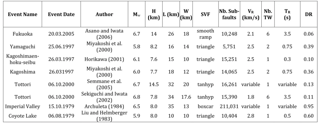
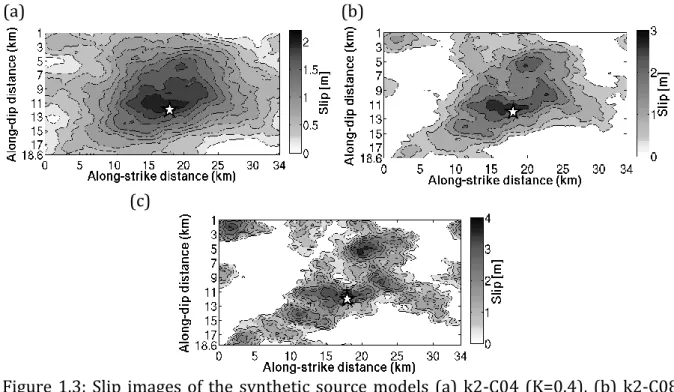
Figure 1.1: Slip images of the kinematic source models, having constant rupture velocity and rise time, extracted from the database of finite-source rupture models and interpolated to a finer grid. The models are (a) Fukuoka (2005), (b) Yamaguchi (1997), (c) Kagoshimaen-hoku-seibu (1997), (d) Kagoshima (1997), (e) Tottori (2000, Sekiguchi and Iwata), (f) Coyote Lake (1979). The symbol ‘star’ shows the location of the hypocenter. Contour lines represent lines of constant slip value. ... 14 Figure 1.2: (a) Slip amplitude, (c) slip duration, (e) rupture front evolution images of Tottori (2000, Semmane et al.), and (b) slip amplitude, (d) slip duration, (f) rupture front evolution images of Imperial Valley (1979). Both kinematic source models have been extracted from the database of finite-source rupture models and then interpolated to a finer grid. ... 15 Figure 1.3: Slip images of the synthetic source models (a) k2-C04 (K=0.4), (b) k2-C08 (K=0.8), (c) k2-C16 (K=1.6), produced using k-2_{descriptions of the final slip. ... 16}

Figure 1.4: Station network for 2005 Fukuoka event with a zoom on the station very close to the fault (at 1, 3 and 10 km distance). The angle θ displayed on the zoomed plot represents the definition of azimuth angle between fault plane and ray path to site, according to Somerville et al. (1997). The radial angles (0° to 180˚) on the top layout represent the alignment direction of the stations at different distances, i.e., the angle between the closest point on the fault and the station. ... 17 Figure 1.5: Synthetic velocity time series on the ‘fault-normal’ component of 2005 Fukuoka source model. Here station azimuth represents the station alignment (the angle between the closest point on the fault and the station) as illustrated in the station layout on the left. ... 19 Figure 1.6: Mean ± std values (bars showing one standard deviation band) of peak ground velocity (PGV) with varying Rjb distances for (a) source models from the

(16)

Figure 1.7: Within-event ground-motion variability () with varying Rjb distances, for

(a) source models from the finite-source rupture model database and (b) k-2_source

models and 2000 Tottori event models. ... 21 Figure 1.8: Mean ± std (bars showing one standard deviation band) of the values of within-event ground-motion variability () with varying Rjb distances, for the cases (i)

bilateral and unilateral events combined (ii) only bilateral events. ... 23 Figure 1.9: PGV values for the stations located at different azimuths along varying Rjb

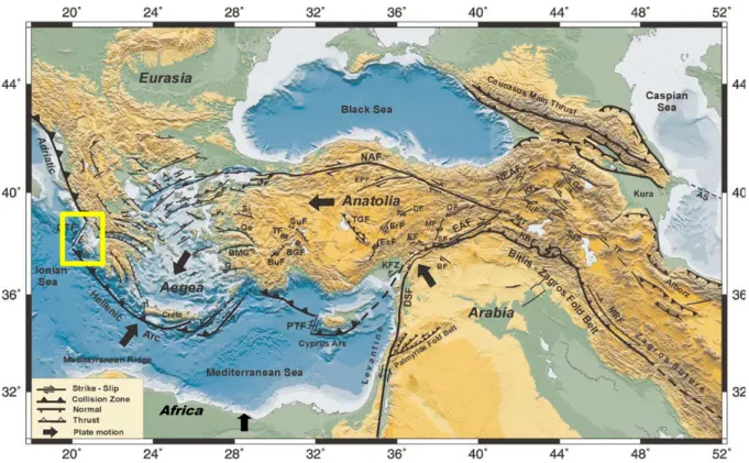
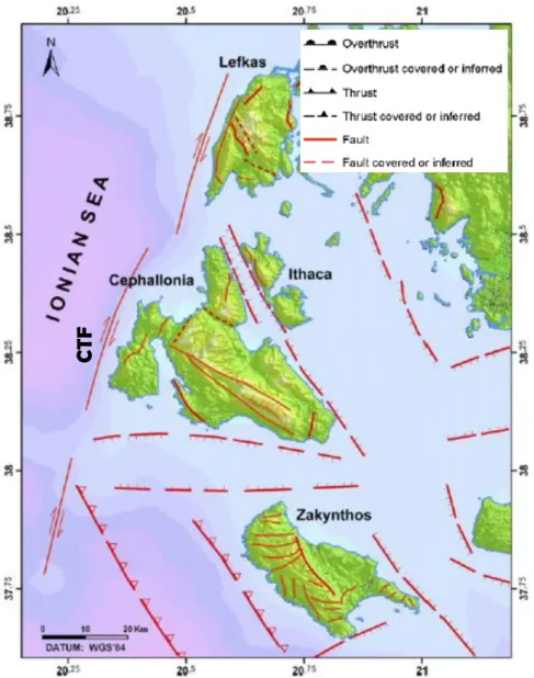
distances, for (a) bilateral and (b) unilateral events. Here azimuth represents θ, the angle between the epicenter and the station, as illustrated in Figure 1.4. ... 25 Figure 2.1: Tectonic-plate map of Greece (Taymaz et al., 2007). Yellow rectangle marks the study area Cephalonia. ... 33 Figure 2.2: Main fault systems of the Cephalonia Island taken from the Seismotectonic Map of Greece (IGME) (Lekkas et al., 2001; Lagios et al., 2007). CTF: Cephalonia Transform Fault. ... 35 Figure 2.3: (a) Shallow seismicity (h ≤ 40 km) in Greece and surrounding region. Yellow rectangle shows Cephalonia area. (Kiratzi et al., 2007; taken from Pitilakis, 2014). (b) Seismotectonic map of Ionian Sea and surrounding area (Papadimitriou et al, 2012). Small circles represent epicentres with Mw > 3.6 for the time period from 1964 to 2005,

large circles labelled 1–10 correspond to historical and instrumentally recorded strong (Mw > 6.0) events before 1964. The fault plane solutions of the events with Mw > 4.5 for

(17)

xiv List of Figures

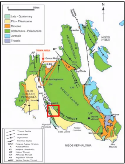
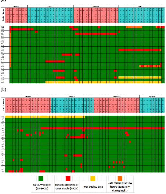
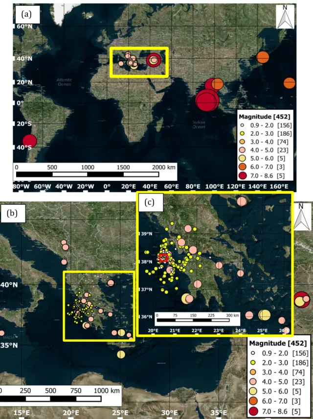
Figure 2.4: (a) The spatial distribution of epicenters of the large past earthquakes for the period 1469-1983 (Papazachos et al. (2000) and (2010); Pitilakis, 2014). (b) Epicenters and the faulting mechanisms of the January 26 and February 3, 2014 earthquakes. Red stars show the epicenters of the two main shocks. Yellow star shows the epicenter of the M = 5.6 aftershock of January 26, 2014 18:45 GMT. The aftershock distribution (M >= 4) of the seismic sequence in Cephalonia one month after the first event are also shown (source: Hellenic Unified Seismological Network-HUSN) The focal mechanisms of these events (source: GCMT solutions) are shown in respective color balloons. The typical focal mechanisms for Cephalonia area (Papazachos and Papazachou, 2003) is shown by the grey ballon. The grey squares and pink triangles denote the sites of accelerographs and seismographs (GEER Report, 2014) ... 38 Figure 2.5: Geological formations of Cephalonia (Underhill, 2006). Red rectangle shows the study area at Argostoli. ... 40 Figure 2.6: Geological formations of Argostoli area, after Lekkas et al. (2001) and modified from Valkaniotis, et al., 2014. Red rectangle shows the study area at Argostoli. ... 40 Figure 2.7: Topographical overview of the test site Argostoli (Hadler et al, 2011). ... 41 Figure 2.8: (a) The SW-NE cross-section and (b) 2D model of the SW-NE section of the Argostoli valley (Protopapa et al., 1998). ... 42 Figure 2.9: H/V average spectral ratios (±1σ) at the center of the valley, site EF2, based on ambient noise recordings of about 1 hour. ... 42 Figure 2.10: Map of fundamental frequency estimated at all the stations from seismological and geophysical investigations carried out by NERA and SINAPSC projects (Boxberger et al., 2014). Black dots indicate sites that do not exhibit any H/V peak. ... 44 Figure 2.11: Location of NERA seismological stations. Circles of different colors indicate the location of the stations. S01, S03, S05, S07 and Array-A constitute the deployed stations by ISTerre. ... 44

(18)

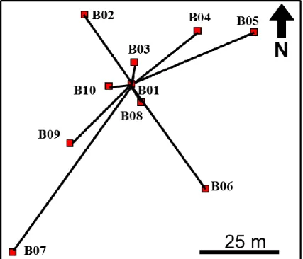
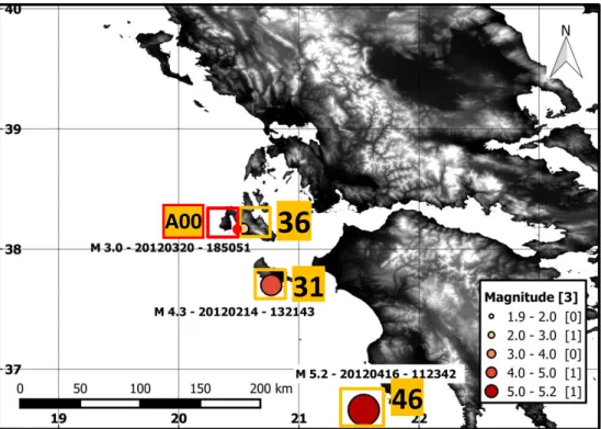
Figure 2.12: Geometry of Array A. A00 is the central station. Stations are located around A00 in four concentric circles at radii 5, 15, 40 and 80 m. Five stations are placed on each concentric circle. The stations branch off from A00 in five directions: N 39, N112, N183, N255 and N 328. ... 45 Figure 2.13: Geometry of Array B. B01 is the central station. Other stations are placed around B01 at distances ranging from 5 to 60 m. ... 46 Figure 2.14: Typical set-up of a station. ... 47 Figure 2.15: A view of central part of the Array A stations. ... 47 Figure 2.16: Day-by-day data availability of ISTerre stations for the period (a) September 2011 to December 2011, and (b) January 2012 to April 2012. ... 48 Figure 2.17: Location of (a) 452 good quality local, regional and teleseismic events. (b) Zoomed in view of the local and regional events from the area marked by yellow rectangle on the (a). (c) Zoomed in view of the events occurring around Argostoli site. Legend on the map represents event locations; the circle-sizes are proportional to the magnitude of the event. The red rectangle on (c) marks the location of the site. ... 50 Figure 2.18: (a) Magnitude and (b) Peak ground velocity (PGV) over the hypocentral distance, and (c) Distribution of peak ground velocity (PGV) of the 452 good quality events. ... 51 Figure 2.19: Map of the analyzed events from (a) Array A (46 events) and (b) Array B (16 events). Catalogue of the events are provided in Appendix F. Orange to red circles (legend) on the map represent event locations; the circle-sizes are proportional to the magnitude of the event. The red circles mark location of the central stations A00 and B01. The events are plotted on SRTM data-maps, available from http://srtm.csi.cgiar.org (Jarvis et al., 2008). ... 53 Figure 2.20: Location of the three example events, no. 36, 31 and 46 in Appendix F.1. Orange rectangles on the map mark the event locations and red one marks the central station A00. ... 54

(19)

xvi List of Figures

Figure 2.21: (a) Velocity time series (b) Fourier amplitude spectra and (c) signal-to-noise ratio, of the three components (EW, NS and UP) recorded at A00 station, for the event no. 36, occurred on March 20, 2012 at UTC 18:50:51. Magnitude, hypocentral depth and epicentral distance of the event are M 3, 18.5 km and 3.1 km, respectively. .. 55 Figure 2.22: (a) Velocity time series (b) Fourier amplitude spectra and (c) signal-to-noise ratio, of the three components (EW, NS and UP) recorded at A00 station, for the event no. 31, occurred on February 14, 2012 at UTC 13:21:43. Magnitude, hypocentral depth and epicentral distance of the event are M 4.3, 13 km and 56 km, respectively. ... 56 Figure 2.23: (a) Velocity time series (b) Fourier amplitude spectra and (c) signal-to-noise ratio, of the three components (EW, NS and UP) recorded at A00 station, for the event no. 46, occurred on April 16, 2012 at UTC 11:23:42. Magnitude, hypocentral depth and epicentral distance of the event are M 5.2, 33 km and 190 km, respectively. ... 57 Figure 3.1: (a) Layout of the Argostoli Array A in the seismological experiment of NERA. (b) Theoretical array response function, and (c) resolution limit: the continuous and dashed black lines, respectively, correspond to the theoretical array resolution limit for the use of classical frequency wavenumber technique, and to half the classical array resolution using high-resolution frequency-wavenumber techniques (Lacoss et al., 1969; Asten & Henstridge, 1984; Cornou et al., 2006; Wathelet et al., 2008). ... 67 Figure 3.2: (a) Layout of the Array B in the seismological experiment of NERA. (b) Theoretical array response function and, (c) resolution limit: the continuous and dashed black lines, respectively, correspond to the theoretical array resolution limit for the use of classical frequency wavenumber technique, and to half the classical array resolution using high-resolution frequency-wavenumber techniques (Lacoss et al., 1969; Asten & Henstridge, 1984; Cornou et al., 2006; Wathelet et al., 2008)... 68 Figure 3.3: Band-pass filtered (1 to 5 Hz) velocity waveforms from (a) vertical component and (b) NS component, recorded across the width of Argostoli valley for an earthquake of M=3.4, Depth = 16.5 km, Back-azimuth=N 134 and Epicentral distance=9 km (event no. 15 in the table in Appendix F.1). Time series recorded at R02 rock site are displayed in red color. Records from R01 station were not available for this event. The corresponding arrangement of the stations on the site is shown at the left. ... 70

(20)

Figure 3.4: Velocity time series of the event no. 12 (ML=3.5) recorded (a) at rock station R02 and (b) at the central station, A00, of Array A. ... 81 Figure 3.5: (a) FAS and (b) SNR for the event no. 12 (ML=3.5) at the central station, A00, of Array A. ... 81 Figure 3.6: Velocity time series of the EW component (top) and spectrogram (bottom) of unfiltered results obtained for the identified dominant waves from array analysis of the event 12. Colorbar represents normalized window energy estimated by Equation 3.26. ... 82 Figure 3.7: Spectrogram of the filtered results from the analysis of event no. 12, when (a) SNR, coherency and slowness filtering is applied and (b) energy filtering is added to the previous filtering. The identified dominant sources characterized as (c) Love (d) Rayleigh (e) retrograde Rayleigh and (d) prograde Rayleigh surface waves from the filtered results. Colorbar represents normalized window energy estimated by Equation 3.26. ... 84 Figure 3.8: Identified back-azimuth distribution of the dominant waves, for event 12, propagating across the Array A. (a) Location of the event with respect to the central station A00. (b) Identified back-azimuths as function of time with colorbar indicating normalized energy as estimated in Equation 3.26. (c) Histogram of identified back-azimuths as a function of frequency with colorbar indicating the summation of normalized energy as estimated in Equation 3.29. Red line indicates the back-azimuth of the event. ... 86 Figure 3.9: Histogram of identified slowness distribution of the dominant waves, for event no. 12, propagating across Array A. Colorbar indicates summation of normalized window energy estimated by Equation 3.30. ... 87

(21)

xviii List of Figures

Figure 3.10: (a) to (h) Distribution of the estimated Love (green dashed line) and Rayleigh (red dashed line) surface-wave normalized energies over 10 degrees back-azimuth interval and various frequency ranges. The blue dot indicates back-back-azimuth of the event. The normalized energies have been estimated by using Equations 3.34 and 3.35. (f) Proportion of identified Love and Rayleigh surface wave energies (Equation 3.25) with respect to the total window energy as a function of frequency. The bar colors, red and green, indicate Rayleigh and Love waves, respectively. ... 90 Figure 3.11: Main results from the analysis of Array B data for event no. 12. (a) Distribution of identified back-azimuths over time. Colorbar shows the normalized energy estimated by Equation 3.26. (b) Histogram of identified back-azimuths over frequency. Colorbar shows the normalized energy estimated using Equation 3.29. Red line indicates the back-azimuth of the event. (c) Histogram of identified slownesses over frequency. Colorbar shows the normalized energy estimated using Equation 3.30. (d) Proportion of identified Love and Rayleigh surface wave energies (Equation 3.25) with respect to the total window energy as a function of frequency. The bar colors, red and blue, indicate Rayleigh and Love surface waves respectively. ... 92 Figure 3.12: Locations of five example events occurred at different directions around the experiment site (Event no. 6, 21, 24, 3 and 7 in Appendix F.1). ... 93 Figure 3.13: Histograms of identified back-azimuths for (a) Array A and (b) Array B data as a function of frequency for five earthquakes occurring in five different back-azimuths (Figure 3.12). Colorbar indicates the summation of normalized energy estimated by Equation 3.29. Red line indicates the back-azimuth of the event. ... 94 Figure 3.14: Proportion of identified Love and Rayleigh surface wave energies (estimated by Equation 3.25) with respect to the total window energy as a function of frequency, for (a) Array A and (b) Array B data. The bar colors, red and green, indicate Rayleigh and Love surface waves, respectively. ... 95

(22)

Figure 3.15: (a) Estimates corresponding to event back-azimuth ± 20° are removed for each event. (b) Then all the estimates from individual events are stacked together to obtain a summary plot. The red line indicates back-azimuth of the event. For all the individual plots, x-axis represents frequency (Hz) and y-axis indicates back-azimuth (degrees). ... 96 Figure 3.16: Overall cumulative distribution for the whole set of events of the diffracted wave field directions for Array A data, after removing the direct arrivals (event back-azimuth ± 20°). Contributions from (a) all waves, (b) Love waves, and (c) Rayleigh waves. Color bar represents the sum of the normalized energy, obtained by Equation 3.36. (d) Direction of dominant diffracted wave arrivals with respect to the array site location. ... 98 Figure 3.17: Overall cumulative distribution for the whole set of events of the diffracted wave field directions for Array B data, after removing the direct arrivals (event back-azimuth ± 20°). Contributions from (a) All waves, (b) Love waves, and (c) Rayleigh waves. Color bar represents the sum of the normalized energy, obtained by Equation 3.36. (d) Direction of dominant diffracted wave arrivals with respect to the array site location. ... 99 Figure 3.18: Overall cumulative slowness distribution for the whole set of events for Array A after removing the direct arrivals (event-back-azimuth ± 20°): (a) For all waves types, (b) Love waves, (c) Rayleigh waves, (d) Retrograde Rayleigh motion and (e) Prograde Rayleigh motion. The color bar represents the sum of normalized energy obtained by Equation 3.37. Black lines represent dispersion curves obtained from classical analysis of ambient noise recorded at Array A and from active surface wave measurements (Boxberger et al., 2014). ... 101 Figure 3.19: Overall cumulative slowness distribution for the whole set of events for Array B after removing the direct arrivals (event-back-azimuth ± 20°): (a) For all waves types, (b) Love waves, (c) Rayleigh waves, (d) Retrograde Rayleigh motion and (e) Prograde Rayleigh motion. The color bar represents the sum of normalized energy obtained by Equation 3.37. Black lines represent dispersion curves obtained from classical analysis of ambient noise recorded at Array B and active surface wave measurements (Boxberger et al., 2014). ... 102

(23)

xx List of Figures

Figure 3.20: Arithmetic mean ±1σ distribution of analyzed energy for Rayleigh and Love waves as function of frequency, after removing the direct arrivals (event-back-azimuth ± 20°) from the estimates of each single event for (a) Array A and (b) Array B. The analyzed energy is expressed as the percentage of the total energy and estimated for each event using Equation 25. Then estimates from all the events are averaged. Red curve corresponds to Rayleigh waves while blue ones to Love waves. Black line shows the mean curve for the total of Rayleigh and Love energy. ... 103 Figure 3.21: Histogram of back-azimuth distribution for event 12 for Array A from (a) the first source and (b) the second source. Red line marks the back-azimuth direction of the event. Colorbar indicates normalized window energy estimated by Equation 3.29. Histogram of slowness distribution for event 12 for (c) the first source and (d) the second source. Colorbar indicates normalized window energy estimated by Equation 3.30. ... 105 Figure 3.22: Histogram of cumulative back-azimuth distribution for Array A for (a) the first source and (b) the second source. Red line marks the back-azimuth direction of the event with colorbar indicating normalized window energy estimated by Equation 3.29. Histogram of cumulative slowness distribution for (c) the first source and (d) the second source with colorbar indicating normalized window energy estimated by Equation 3.30. ... 107 Figure 3.23: Histogram of back-azimuth distribution for event 12 from Array-B data for (a) the first source and (b) the second source. Red line marks the back-azimuth direction of the event. Colorbar indicates normalized window energy estimated by Equation 3.29. Histogram of slowness distribution from (c) the first source and (d) the second source. Colorbar indicates normalized window energy estimated by Equation 3.30. ... 108 Figure 3.24: Histogram of cumulative back-azimuth distribution for Array B for (a) the first source and (b) the second source. Colorbar indicates normalized window energy estimated by Equation 3.36. Histogram of cumulative slowness distribution for (c) the first source and (d) the second source. Colorbar indicates normalized window energy estimated by Equation 3.37. ... 109

(24)

Figure 3.25: Ensemble of inverted shear-wave velocity profiles that explain the observed dispersion data within their uncertainty bound at (a) Array A and (b) Array B. Group velocities computed from the ensemble of shear-wave velocity profiles for the first 5 modes of Rayleigh (black lines) and Love (gray lines) waves for (c) Array A and (d) Array B. Mean ±1σ distribution of the cumulative analyzed energy for (e) Array A and (f) Array B (see Figure 3.20 for details). ... 111 Figure 3.26: Comparison of estimated standard spectral ratio (SSR) with wave type and wave energy repartition for Array A. (a) Standard spectral ratio (SSR) from the horizontal components of A00 and R02 stations obtained by averaging SSRs from 164 events (Cultrera et al., 2014). Black line shows the geometric mean of SSR and grey-shaded region indicates ±1σ. (c) Mean ±1σ distribution of the cumulative analyzed energy for Array A as shown in Figure 3.20 (a). Histogram of back-azimuth distribution as a function of frequency for (b) Love and (d) Rayleigh waves as also shown in Figure 20 (b) and (c), respectively. In (b), (c) and (d) blue and red arrows and rectangle indicate frequency range dominated by Love and Rayleigh waves, respectively. ... 113 Figure 3.27: Comparison of estimated standard spectral ratio (SSR) with wave type and wave energy repartition for Array B. (a) Standard spectral ratio (SSR) from the horizontal components of KES04 and R02 stations obtained by averaging SSRs from 164 events (Cultrera et al., 2014). Black line shows the geometric mean of SSR and grey-shaded region indicates ±1σ. (c) Mean ±1σ distribution of the cumulative analyzed energy for Array B as shown in Figure 3.20 (b). Histogram of back-azimuth distribution as a function of frequency for (b) Love and (d) Rayleigh waves as also shown in Figure 20 (b) and (c), respectively. In (b), (c) and (d) blue and red arrows and rectangle indicate frequency range dominated by Love and Rayleigh waves, respectively. ... 114 Figure 4.1: Illustration of the physical causes underlying the spatial variation of the seismic ground motion. The different parts of the figure show schematically (a) the wave passage effect, (b) the extended source affect (c) the scattering effect. The graphic illustrations are presented after Zerva (2009). ... 126 Figure 4.2: Typical shapes of (a) auto spectral density function, (b) absolute coherency, (c) wrapped phase, and (d) unwrapped phase, after Harichandran (1999). ... 130

(25)

xxii List of Figures

Figure 4.3: Example of an 11-point (Mh=5) Hamming Window ... 134

Figure 4.4: The bias and standard deviation of the coherency smoothing for different Hamming window frequency weights and a 1000 point 5% double cosine taper data window, after Abrahamson (1992b). ... 137 Figure 4.5: Example of the 50% and 90% confidence levels for different Hamming window frequency weights for (a) tanh − 1|γjkω| and (b) |γjkω|, after Abrahamson (1992b). ... 137 Figure 4.6: Layout of Array A in the seismological experiment at Argostoli. Distance between the rock stations R01 and R02 is about 2 km. The central station of the array, A00, is located about 550 m away from R02 station in the northeast and 450 m away from the southwest edge of the valley. ... 139 Figure 4.7: Magnitude-distance distribution of the selected subset of events ... 140 Figure 4.8: Duration of the selected time windows, from 46 events, plotted against the hypocentral distances of the respective events. The colorbar represents the magnitude of the events. ... 141 Figure 4.9: Time windows from the rock-stations based on normalized Arias Intensity estimations for the 46 events. ... 143 Figure 4.10: Comparison between the time windows based on visual inspection and AI method, from the rock-stations. ... 144 Figure 4.11: Comparison between the time windows from rock (R01, R02) and sedimentary (A00) stations based AI method. ... 144 Figure 4.12: Time series of the horizontal components from (a) R02 and (b) A00 for the event no. 5 (Appendix F). The red segment of signal shows the visual selection on R02 seismogram (66.5-67 s) and corresponding window on A00. The brackets on R02 and A00 seismogram show the selections from AI-method on rock (66.5- 67.3 s) and sediment (66.7-67.6 s), respectively. ... 145

(26)

Figure 4.13: Time series of the horizontal components from (a) R02 and (b) A00 for the event no. 8 (Appendix F). The red segment of signal shows the visual selection on R02 seismogram (89- 95 s) and corresponding window on A00. The brackets on R02 and A00 seismogram show the selections from AI-method on rock (90.5-97 s) and sediment (95.5-100.8 s), respectively. ... 146 Figure 4.14: Time series of the horizontal components from (a) R02 and (b) A00 for the event no. 46 (Appendix F). The red segment of signal shows the visual selection on R02 seismogram (115.6-129.8s s) and corresponding window on A00. The brackets on R02 and A00 seismogram show the selections from AI-method on rock (131.9-142.5 s) and sediment (131.4-137.2 s), respectively. ... 147 Figure 4.15: Comparison of the durations, estimated based on (a) rock station records using method and visual inspection (b) rock and sediment station records using AI-method. Blue lines show the ±10% band of error. Colorbar shows the hypocentral distance. ... 148 Figure 4.16: The lagged coherency estimation between the stations I12 and C00-I06 for the Event-5 recorded by SMART-1 array. (a) Results of the estimation from this study (b) Results from Zerva (2009). ... 152 Figure 4.17: (a) Array A geometry, (b) velocity time series of event no. 46 (Appendix F) and (c) sensitivity of estimated lagged coherency to duration of selected time window. The plots represent the estimated coherency (EW component) between A00 and the stations on the 15m-radius circle of the Array A. The time histories from R01 are given in Figure 4.14 (a). The colorbar ‘Test ID’ indicates the index of the test time windows. Test 1 to 4 consider 4 different lengths (116-130s, 116-138s, 116-142s, 116-150s) of time windows starting from the begin time identified by visual inspection of R02. Test 5 and 6 consider two different lengths (132-142s, 132-150s) with respect to the automatic time window estimation from R02 records. ... 154 Figure 4.18: (a) Time history, (b) Fourier amplitude spectra and (c) signal to noise ratio for the event occurred on October 9, 2011 at 18:42:20 UTC (M=3.3, Rhyp=93.3 km, Baz=

N 117, tw=5.88s). The event index is 8 in Appendix F. Red segment on the time history plot marks the window used for coherency estimation. ... 156

(27)

xxiv List of Figures

Figure 4.19: (a) Array configuration angle at N39 and (b) Lagged coherency (EW component) at interstation angle N39 for 4 inter-station distances (event no. 8). The black arrow shows the event back-azimuth. ... 157 Figure 4.20: Lagged coherency variability (EW component) of event no 8. Each plot represents 4 interstation distances for the pairs lying in 5 array-branch directions. ... 157 Figure 4.21: (a) Array configuration for 5 array directions and (b) Lagged coherency (EW component) of event no 8 at 5 array directions for inter-station distance 15m. The black arrow shows the event back-azimuth. ... 158 Figure 4.22: Lagged coherency variability (EW component) of event no 8. Each plot represents station pairs lying in 5 array branch directions at 4 interstation distances. ... 158 Figure 4.23: (a) Array configuration, (b) valley cross-section and (c) lagged coherency variability (EW component) from the events (M~3.1, Baz~ N220) with different hypocentral distances, at 5 array directions (indicated on the top of each panel) and 4 interstation distances (indicated at the left of each row of figures). Legend indicates the hypocentral distances. ... 161 Figure 4.24: (a) Array configuration, (b) valley cross-section and (c) lagged coherency variability (EW component) for the events (M~2.8, Rhyp~20km) from different

back-azimuths, at 5 array directions (indicated on the top of each panel) and 4 inter-station distances (indicated at the left of each row of figures). Legend indicates the event back-azimuths. ... 162 Figure 4.25: (a) Array configuration, (b) valley cross-section and (c) lagged coherency variability (EW component) of the events (Rhyp~20km, Baz~N 220) with different

magnitudes, at 5 array directions (indicated on the top of each panel) and 4 inter-station distances (indicated at the left of each row of figures). Legend indicates the magnitudes of the events. ... 163 Figure 4.26: (a) Array configuration, (b) valley cross-section and (c) lagged coherency variability (EW component) with increasing interstation distances for different frequencies, at 5 array directions. ... 164

(28)

Figure 4.27: ATANH median curves of 46 events from the time windows selected visually from rock stations. The thick red curve shows the ‘global median’. Dij stands for interstation distance and EW, NS, Z stand for the ground-motion components. Blue line marks the coherency resolvability threshold. ... 168 Figure 4.28: ATANH Coherency residuals of ‘individual median’ estimates with respect to the ‘global median’, from the time windows selected visually from rock stations. Dij stands for interstation distance and EW, NS, Z stand for the ground-motion components. ... 169 Figure 4.29: Distribution of ATANH estimates of 46 events (EW component), from the time windows selected visually from rock stations, at different distance and frequency ranges (indicated at the left of each row of figures). Red line shows the coherency resolvability threshold. Dij stands for interstation distance... 170 Figure 4.30: Global median estimates of lagged coherency from three different time-window selection approaches. Red, green and blue curves indicate the time time-windows selection from visual inspection on rock, AI-based estimation on rock and AI-based estimation on A00, respectively. Dij stands for interstation distance and EW, NS, Z stand for the ground-motion components. Blue line marks the coherency resolvability threshold. ... 171 Figure 4.31: Comparison between horizontal components for (a) EW and NS, (b) valley-perpendicular (N40) and valley-parallel (N130), and (c) radial (baz-parallel) and transverse (baz-perpendicular) components of the ground motion, with their respective 85% confidence interval bound. On each figure, red and blue curves indicate the horizontal components and magenta and cyan curves indicate the respective 85% CI intervals. Dij stands for interstation distance. Blue line marks the coherency resolvability threshold. ... 173 Figure 4.32: Comparison among horizontal components from different orientation definitions. On each figure, red, green and blue curves indicate EW, valley-perpendicular and baz-perpendicular components, respectively. Dij stands for interstation distance. Blue line marks the coherency resolvability threshold. ... 174

(29)

xxvi List of Figures

Figure 4.33: Graphic representation of (a) five array-branch directions (arrows in five colors), (b) orientation of horizontal ground-motion components (red small arrows indicate valley perpendicular and blue small arrows indicate valley-parallel orientations) and, (c) valley axes. ... 175 Figure 4.34: Comparison of median coherencies among the five directions of the array-branches for valley-perpendicular (N40), valley-parallel (N130), and vertical components. Dij stands for interstation distance, ‘Comp’ stands for the component of ground motion. Blue line marks the coherency resolvability threshold. ... 175 Figure 4.35: Comparison of median coherencies between Valley-perpendicular and Valley-parallel pairs for valley-perpendicular (N40), valley-parallel (N130) and Z components. Magenta and cyan curves indicate the corresponding 85% CI intervals. Dij stands for interstation distance comp stands for the component of ground motion. Blue line marks the coherency resolvability threshold. ... 176 Figure 4.36: Global median estimates of ATANH coherency for the event back-azimuth oriented station pairs. Blue and red curves indicate the perpendicular and baz-parallel pairs, respectively. Magenta and cyan curves indicate the respective 85% CI intervals Dij stands for interstation distance, comp stands for the component of ground motion. Blue line marks the coherency resolvability threshold. ... 178 Figure 4.37: Comparison of unlagged ATANH coherency estimations from S- and coda wave windows Dij stands for interstation distance and N40, N130, Z stand for the ground-motion components. Blue line marks the coherency resolvability threshold. . 179 Figure 4.38: Global median estimates of ATANH coherency from coda wave window for the valley-axis oriented station pairs. Blue and red curves indicate the valley-parallel and valley-perpendicular pairs, respectively. Magenta and cyan curves indicate the respective 85% CI intervals Dij stands for interstation distance, comp stands for the component of ground motion. Blue line marks the coherency resolvability threshold.180 Figure 4.39: Residuals of ATANH coherency curves for the Valley-perpendicular component of the events coming from Rhyp 0-60km. ... 181

(30)

Figure 4.40: Residuals of ATANH coherency curves for the Valley-perpendicular component of the events coming from Rhyp 60-200km. ... 182

Figure 4.41: Residuals of ATANH coherency curves of the Valley-perpendicular component for the M 2-3 events. ... 183 Figure 4.42: Residuals of ATANH coherency curves of the Valley-perpendicular component for the M 3-5 events. ... 184

(31)

xxviii List of Symbols/Abbreviations

List of Symbols/Abbreviations

γ̅_jk(ω) Lagged coherency or coherency

δ residual

Δ steps

θ Azimuth angle (Chapter 1), back-azimuth angle (Chapter 3, 4) ρ Amplitude parameter

σtot Total ground motion variability (sigma)

σSS Single station sigma

Σ summation

τ Between-event variability (Chapter 1), time (Chapter 4) φ Phase difference (Chapter 3)

ϕ Within-event variability

ϕSS Event corrected single station sigma

ω Angular frequency ωm Frequency smoothed

a Steering vector of MUSIC functional am Weight of frequency smoothing

aq Modified steering vector of MUSIC functional

ATANH, tanh-1

Hyperbolic arc tangent

Dij Separation distance between stations i and j

E Expectation value

EXX Energy; XX = different components

f frequency fc Central Frequency fs Sampling frequency FK Frequency-wavnimuber H, h Hypocentral depth H/V Horizontal/Vertical Im Imaginary part

(32)

k Wave number

kc Corner wave number

K Degree of slip heterogeneity (Chapter 1), Number of strongest eigenvalues (Chapter 3)

l Time sample

L Length of fault

Lc Characteristic rupture length

m Time index

M Earthquake magnitude

Mh Number of points of Hamming window

ML Local magnitude

Mw Moment magnitude

n Number of observations N Number of sensors/signals Nf Number of frequency points

Nt Number of time index

Nst Number of stations

P MUSIC functional q Quantile value R, r Epicentral distance

R Matrix of sensor position Re Real part

Rhyp Hypocentral distance

Rjb Joyner-Boore distance

Rrup Rupture distance

s Site category (Chapter 1), slowness (Chapter 3) S(f) Single covariance matrix

S̅_jj Smoothed auto power spectrum for station j

S̅jk Smoothed cross power spectrum between stations j and k

tc Centre of time window

Tp Time of peak velocity

(33)

xxx List of Symbols/Abbreviations U(l) Ground motion time series U(ω) Ground motion Fourier spectrum X Complex data vector

TR Rise Time

v Velocity of wave VR Rupture velocity

Vs Shear wave velocity W Width of fault

AI Arias Intensity

AUTH Aristotole University of Thessaloniki BC Before Christ

BSSA Bulletin of the Seismological Society of America CI Confidence Interval

CTF Cephalonia Transform Fault DR Directivity Ratio

EMSC European‑Mediterranean Seismological Centre EU European Union

FAS Fourier Amplitude Spectum GCMT Global Centroid Moment Tensor

GFZ German Research Centre for Geosciences GIS Geographical Information System

GMPE Ground Motion Prediction Equation GMT Greenwich Mean Time

GPS Global Positioning System

HUSN Hellenic Unified Seismological Network InSAR Interferometric Synthetic Aperture Radar INGV Istituto Nazionale Geofisica e Vulcanologia ISTerre Institut des Sciences de la Terre

ITSAK Institute of Engineering Seismology and Earthquake Engineering (Greece) MUSIC MUltiple SIgnal Characterization

(34)

NE North East

NERA Network of European Research Infrastructures for Earthquake Risk Assessment and Mitigation

PGV Peak Ground Velocity NW North West

PSHA Probabilistic Seismic Hazard Assessment SE South Easr

SNR Signal to noise ratio SSR Standard Spectral Ratio SVF Slip velocity function

SVEGM Spatial Variation of Earthquake Ground Motion SW South West

(35)

(36)

General Introduction

Earthquake has been one of the deadliest natural hazards throughout the history of human civilization. In a seismically active region, ground shaking caused by earthquakes pose inevitable risk to the inhabitants and infrastructure subjected to it. To date, a number of urban centers have been developed near major earthquake faults. The trend of growing urbanization has been followed by the construction of significant numbers of large and extended structure. Hence, one key challenge in modern day engineering practices is to better understand the processes associated with ground shaking in order to mitigate the effects and to cope with the future earthquakes.

An earthquake occurs when rocks slip suddenly due to the stresses built up in the earth’s outer layer. Energy radiates away from the source of this sudden movement and propagates as seismic waves rapidly through the earth’s crust reaching the ground surface where they produce shaking, i.e. the ground motion. Accordingly, the factors that influence ground motion during earthquakes are attributed to the complexity of the source, propagation path, and site effects. Seismologists and engineers base their understanding on knowledge of these effects in order to estimate as well as to predict the level and nature of ground motion.

Generally speaking, the damage caused by earthquakes depends on the strength or intensity of the ground motion coupled with the quality of the engineering structure. The level of shaking is controlled by the proximity of the affected region or structure to the earthquake source as well as the type of geological structure that seismic waves pass through en route, especially those at or near the ground surface. On their travel path, seismic waves make their final way through the ground structure near the surface where they are greatly modified by the local geology and soil conditions. When the waves pass from rock to soil, they slow down in propagation speed but become larger in amplitude. The more intense shaking of the sedimentary layers cause greater energy movement and results in larger waves. Since geometry and soil conditions of the sedimentary layer often vary over short distances, nature and levels of ground shaking can vary significantly within a small area.

(37)

2 General Introduction

As a matter of fact, a number studies have reported large variations in the spatial distribution of ground motion during past major damaging earthquakes (e.g. Shabestari and Yamazaki, 2003). The degree of damage was often observed to vary from one location to another, even for similar structures located within short distances, which consistently suggest different levels of ground motion in addition to vulnerability variations linked with structural defaults. Some important issues raised by recent earthquakes and requiring elucidations are therefore:

- How do the seismic waves, radiated from the source, affect ground motion variability in the near-fault region?

- What are the physical properties of the source that contribute to this variability? - To what extent is ground motion variability caused by the local geological

structure?

- What type or characteristics of the seismic waves modify the nature and level of ground motion in such sites and within short distances?

Answering such issues is obviously required to improve our understanding of such complex source and site effects through a mix of experimental observations and numerical simulations.

By definition, spatial variation of earthquake ground motion refers to the differences in amplitude and waveform (phase) observed in the seismic time histories recorded over extended areas (e.g. within the dimension of a engineered structure) on the ground surface. It has significant effect on the dynamic response of engineered structures with large dimensions, such as dams, nuclear power plants, or multiple supports such as bridges and lifeline facilities. Usually, spatially uniform ground motion excitation is assumed in practice for seismic analysis. This assumption becomes inadequate for spatially extended structures constructed in the near-fault region or on large sites with inhomogeneity in surface geology and geometry, emphasizing the need to include spatial variability in earthquake-resistant design and analysis of such structures.

The effect of source characteristics on the ground motion is profound. In the near-fault region, shallow earthquakes can cause severe differences in ground motions depending on the direction of the fault rupture. The existing Empirical Ground Motion Prediction Equations (GMPEs) provide the distribution of ground-motion in terms of a median and

(38)

a standard deviation, but these equations are developed by means of regression techniques from recorded strong motion data, generally based on very simple parameterization with magnitude, distance and site category. On the other hand, the standard deviation of the ground motion distribution, commonly referred to as the aleatory variability “sigma”, is a fundamental component in Probabilistic Seismic Hazard Assessment (PSHA) since it controls the hazard level at very low probabilities of exceedance. It is therefore imperative to accurately constrain “sigma” to perform reliable seismic hazard analyses. Though a few recent data analyses suggest that sigma is distance-dependent, development of models describing ground motion variability at short distances (<20 km) remains questionable due to the scarcity of near-source records of moderate to large events (Mw>6).

Furthermore, it is well known that engineering structures cross sites with irregular subsurface topography and ground types (e.g. sedimentary valleys). Such sites give rise to the formation of surface waves, which can lead to large amplifications, loss of correlation and significant ground strains in the wave field. Besides, seismic waves become trapped and amplified by sedimentary valleys during earthquakes. As a result strong ground motion of long duration and strong spatial variation in amplitude and phase occur, especially near the edges of the basins, which can substantially increase the seismic forces on structures and lifelines. Such effects could not be incorporated so far in routine seismic hazard assessment and risk mitigation due to their complexity as well as the limitations of geophysical investigations. The installation of dense seismic arrays worldwide initiated the comprehensive analysis of seismic ground motion. However, most of these arrays are located at uniform ground conditions, mostly at soil sites. In addition, most of the array analysis studies utilized a stochastic approach (coherency estimation) to model the spatial variation of the motions (Zerva, 2009). A purely stochastic approach, however, precludes any association of the spatial variation of the motions with the physical causes underlying it. Additional research efforts at such sites are, hence, necessary to fully capture the physical causes underlying the spatial variation of the seismic ground motions for engineering applications.

One of the main (long term) goals of this thesis is, then, to understand the key parameters that locally control the ground motion spatial variability, as well as to

(39)

4 General Introduction

investigate the relative contributions of scattering and local site effects, in view of aiding development and calibration of engineering oriented models, and to put forth practical propositions for incorporating the effects of such a variability in seismic design (building codes, microzonation studies, critical facilities). It includes two main parts. The first one addresses the spatial "aleatory" variability of ground motion related to the aleatory features of rupture kinematics in the near fault region, while the second one is dedicated to an analysis of the variability of ground motion over short distances in connection to the shallow underground structure at the site : although such a variability is usually considered as stochastic, our goal here is to investigate its "deterministic" relationship with the composition of the wave field, which includes both source and site signatures. The first part of the thesis is based on numerical simulations while the second on recorded data.

The PhD thesis begins with the analysis of potential distance dependency of the ground-motion variability “sigma” (chapter 1). The main goal is to quantify statistical properties of ground-motion variability in the near source region where it is poorly constrained due to the lack of available records, and look into the relative contributions of source complexity and wave propagation effects. Therefore, numerical simulations of ground motions were performed for strike-slip events. Synthetic velocity seismograms have been generated from a suite of finite-source rupture models of past earthquakes. Then the within-event component of the ground-motion variability, in terms of variance in peak ground velocity (PGV), was evaluated as a function of distance.

The second, experimental, part of the thesis deals with the identification of seismic wave field composition in a site with pronounced shallow underground heterogeneities, with the objective to improve the physical understanding and the engineering-oriented quantification of spatial variability of ground motion (i.e. spatial coherency). This part of the research is based on the temporary seismological experiment that took place at the Argostoli basin within the FP7 EU-NERA (Network of European Research Infrastructures for Earthquake Risk Assessment and Mitigation) 2010-2014 project. The chosen site Koutavos-Argostoli area is a relatively small-size shallow sedimentary basin, situated in the Cephalonia Island, Western Greece, where the seismic activity is high and dominated by the Cephalonia transform fault (chapter 2). The seismological wave field

(40)

generated by a significant number of earthquakes was investigated from dense array recordings of earthquake ground motion using an array analysis technique MUSIQUE (Hobiger et al., 2012) (chapter 3). Unlike the classical array processing methods (high-resolution frequency-wavenumber analysis [Capon, 1969], MUSIC [Schmidt, 1986]), MUSIQUE allows analysis of all three components of a seismic record together and identification of the surface wave types as well as retrieval of wave polarization along with resolving the wavenumber vector. Thus the results from MUSIQUE analysis provide us with slowness and back-azimuth of the dominant wave trains crossing the array, discrimination between Rayleigh and Love surface waves, plus, estimates of polarization parameters of Rayleigh waves.

Subsequently, the "lagged coherency" of the ground motion has also been quantified for each possible pair within the array and for the set of selected events (chapter 4). This work focuses on observation of spatial variation of the waveforms over short distances, that is, within the dimension of a large structure. The final goal is to associate lagged coherency with the results obtained from wave field characterization and investigate the dependency of coherency on source parameters (such as magnitude, distance, source direction) as well as the site parameters (such as azimuth of station pairs, basin axis) based on statistical analyses.

The last section wraps up the main findings from each of the three major components of this work concerning the spatial variability of ground motion: even if it is most often described as stochastic, it does include some deterministic items. It thus identifies some perspectives that now seem at hand, given the data and results obtained here. The appendix gathers information that is not critical for the understanding of the main chapters, but may be of interest to curious readers or all those who would perform some similar studies or use the same data set for other purposes.