HAL Id: tel-02418670
https://tel.archives-ouvertes.fr/tel-02418670v2
Submitted on 2 Apr 2020
HAL is a multi-disciplinary open access
archive for the deposit and dissemination of sci-entific research documents, whether they are pub-lished or not. The documents may come from teaching and research institutions in France or
L’archive ouverte pluridisciplinaire HAL, est destinée au dépôt et à la diffusion de documents scientifiques de niveau recherche, publiés ou non, émanant des établissements d’enseignement et de recherche français ou étrangers, des laboratoires
Knot theory and cluster varieties
Nicolas Pastant
To cite this version:
Nicolas Pastant. Knot theory and cluster varieties. Rings and Algebras [math.RA]. Université de Strasbourg, 2019. English. �NNT : 2019STRAD053�. �tel-02418670v2�
ÉCOLE DOCTORALE MSII ED269
IRMA, UMR 7501
THÈSE
présentée par :
Nicolas PASTANT
soutenue le :
20 décembre 2019pour obtenir le grade de :
Docteur de l’université de Strasbourg
Discipline/ Spécialité
: Mathématiques fondamentales
Théorie des nœuds et variétés
amassées
THÈSE dirigée par :
M. FOCK Vladimir Professeur, Université de Strasbourg
RAPPORTEURS :
M. TUMARKIN Pavel Professeur, Durham University
M. ITENBERG Ilia Professeur, Université Pierre et Marie Curie
AUTRES MEMBRES DU JURY :
M. BAUMANN Pierre Chargé de recherches HDR, Université de Strasbourg
Théorie des nœuds et
Variétés amassées
Nicolas Pastant
Institut de Recherche Mathématique Avancée
Université de Strasbourg
7 rue René Descartes
67084 Strasbourg Cedex
Thèse de doctorat sous la direction de
Vladimir Fock
Contents
Introduction 1 1 Cluster varieties 5 1.1 Cluster X -manifolds . . . 5 1.1.1 Definitions . . . 5 1.1.2 Amalgamation . . . 61.2 Thurston diagrams and embedded bipartite graphs . . . 7
1.2.1 Thurston diagrams . . . 7
1.2.2 Bipartite graphs . . . 8
1.2.3 Relation between Thurston diagrams and bipartite graphs . . . . 9
1.3 Cluster X -manifolds constructed from a Dynkin diagram . . . 9
1.3.1 Cluster X -varieties related to the braid semigroup . . . 10
1.3.2 Cluster X -varieties related to the Hecke semigroup . . . 11
1.3.3 The evaluation map . . . 12
1.3.4 Properties of the spaces XB . . . 12
1.4 AnCluster X -manifolds . . . 13
1.4.1 Thurston diagrams and cluster varieties associated to P GLn(C) . 14 1.5 AbnCluster X -manifolds . . . 15
1.5.1 The coextended affine Weyl group . . . 15
1.5.2 The Laurent realisation of the group dP GL#n(C) . . . 16
1.5.3 The Thurston diagram description . . . 17
1.5.4 The evaluation map . . . 18
2 Links and braids 19 2.1 Links . . . 19
2.2 Milnor Torsion of link exteriors . . . 20
2.2.1 Torsion of chain complexes . . . 20
2.2.2 Milnor torsion of link exteriors . . . 21
2.3 Braids . . . 22
2.3.2 Colored oriented braids groupoid . . . 24
2.3.3 Annular braid group . . . 24
2.3.4 Colored oriented annular braids groupoid . . . 25
2.4 Burau representations . . . 25
2.4.1 The Burau representations of colored oriented Artin braids . . . . 25
3 Cluster manifolds associated to links, braids and their invariants 27 3.1 Dimer model for the torsion of link exteriors . . . 27
3.1.1 Introduction . . . 27
3.1.2 A CW-complex structure on a link complement . . . 28
3.1.3 Graph encoding the cellular structure . . . 30
3.1.4 Weighting on the graph . . . 31
3.1.5 Computation of the torsion of the link exterior . . . 32
3.2 Burau cluster submanifolds associated to braids . . . 33
3.2.1 Burau cluster submanifolds associated to oriented colored braids, the reduced case . . . 34
3.2.2 Demonstration of theorem 3.1 . . . 36
3.2.3 Burau cluster submanifolds associated to oriented colored braids, the unreduced case . . . 43
3.2.4 Demonstration of theorem 3.2 . . . 45
3.3 Burau cluster submanifolds associated to annular braids . . . 51
3.3.1 Burau cluster submanifolds associated to oriented colored annu-lar braids, the reduced case . . . 52
3.3.2 Demonstration of theorem 3.3 . . . 53
3.3.3 Burau cluster submanifolds associated to oriented colored annu-lar braids, the unreduced case . . . 53
3.3.4 Demonstration of theorem 3.4 . . . 54
Introduction
Le but de cette thèse est de donner de nouvelles applications de la théorie des variétés amassées à la théorie des nœuds, ou plus généralement à la topologie des variétés de dimension 3.
Motivés par l’étude de la positivité totale et des bases canoniques dans les groupes quantiques, Fomin et Zelevinsky [FZ02] ont introduit les algèbres amassées au début des années 2000. Les variétés amassées introduites par Fock et Goncharov [FG06a] sont des analogues géométriques des algèbres amassées. Elles apparaissent naturellement dans le contexte de la théorie de Teichmüller [FG07]. La combinatoire des algèbres et variétés amassées joue un rôle important dans de nombreux domaines. Nous citons en particulier : physique statistique [GK11] , théorie de Lie [FG06b], géométrie de Poisson [GSV03] et systèmes dynamiques discrets [KNS11].
La théorie des nœuds dont l’origine remonte aux travaux de Gauss sur l’indice d’entre-lacement au 19e sciècle est, elle aussi, liée à de nombreux domaines des
mathéma-tiques et de la physique. Les travaux de Jones [Jon85] ont notamment donné lieu au développement de la topologie quantique. Il est remarquable que, dans ce contexte, certains invariants de nœuds peuvent être exprimés comme fonction de partition de modèles issus de la mécanique statistique [Kau06]. De même, les groupes de tresses et certaines de leurs généralisations peuvent être interprétés du point de vue de la théorie de Lie [All02].
L’objectif de notre travail est de montrer que certains invariants de nœuds et tresses peuvent être exprimés comme des invariants de variétés amassées naturellement asso-ciés à des représentants diagrammatiques de ces objets topologiques.
Dans le premier chapitre nous rappelons, dans le paragraphe 1.1 les définitions des variétés amassées de Fock et Goncharov [FG06b] dans le cas particulier qui nous in-teresse, à savoir les variétés amassées de type X dans le cas simplement lacé et où le corps de base est C. Dans ce cas ce sont des variétés complexes obtenues par recolle-ment de tores algébriques (C∗)navec n fixé et où les applications de recollement sont des applications birationnelles appelées mutations dont la forme est définie de manière
précise à partir d’une matrice symétrique. Ces variétés sont munies d’une structure de Poisson. Nous présentons en particulier deux classes de variétés amassées dans le sens précédent.
• Les graphes bipartis plongés cellulairement dans une surface étudiés par Gon-charov et Kenyon [GK11] que nous présentons dans le paragraphe 1.2.2
• Les variétés amassées construites à partir d’un diagramme de Dynkin par Fock et Goncharov [FG06b] présentées dans le paragraphe 1.3
Dans les paragraphes correspondants, nous rappelons la construction des invariants de ces variétés, la fonction de partition de dimères dans le premier cas et l’application d’évaluation dans le second. Dans le cas particulier des diagrammes des séries A et ˆA, la seconde classe de variétés amassées est décrite par Fock est Marshakov [FM14] à l’aide de diagrammes introduits par Thurston [Thu04]. Cette description est rappelée dans le paragraphe 1.4 dans le cas de la série A et dans le paragraphe 1.5 pour la série
ˆ A.
Dans le second chapitre nous donnons les définitions des objets de la théorie des nœuds que nous étudions ainsi que leurs invariants que nous réinterprétons du point de vue des variétés amassées, à savoir, dans le paragraphe 2.2, la torsion de Milnor-Turaev de l’extérieur des entrelacs et deux méthodes de calcul de cette dernière : la méthode des τ -chaînes de Turaev [Tur86] et la méthode des contractions de chaînes. Nous rappelons dans le paragraphe 2.4 les définitions des groupoïdes des tresses colorées orientées dans les cas planaires et cylindriques ainsi que les représentations de Burau réduites et non réduites de ces groupoïdes [Bur35] [SW01] [GTW17].
Le chapitre 3 constitue le cœur de cette thèse dans lequel nous présentons et démon-trons nos résultats :
• Nous étendons et interprétons géométriquement le modèle de dimères pour le polynôme d’Alexander de Cohen, Dasbach et Russel [CDR14]. À partir d’un dia-gramme d’entrelacs nous construisons dans le paragraphe 3.1.3 un graphe biparti qui encode une structure cellulaire sur l’extérieur de l’entrelacs relativement à son bord. Nous décrivons dans le paragraphe 3.1.4 une pondération de ce graphe qui encode un système de coefficients locaux induit par le morphisme d’abélianisation du groupe fondamental de l’entrelacs. Cette donnée nous permet de décrire dans le paragraphe 3.1.5 la torsion de Milnor de l’extérieur d’un entrelacs comme une fonction de partition de dimères.
• Dans le paragraphe 3.2 nous associons aux tresses colorées orientées classiques des sous-variétés des variétés amassées construites à partir du digramme de Dynkin de type A. En composant avec l’application d’évaluation nous obtenons une
Introduction
représentation du groupoïde des tresses colorées orientées classiques. Pour la représentation standard de P GLn(C) nous obtenons les matrices de la
représen-tation de Burau réduite pour une version de notre construction, et celle de la représentation de Burau non réduite pour une version en un certain sens duale. • Nous décrivons dans le paragraphe 3.3 une construction similaire au point
précé-dent pour le groupoïde des tresses colorées orientées cylindriques. Les variétés amassées impliquées sont dans ce cas, celles construites à partir des diagrammes de Dynkin de type ˆA.
On peut résumer nos résultats dans le tableau suivant : Objet noué Variétés amassées
associées
Invariant amassé correspondant
Invariant de l’objet noué Entrelacs dans S3 Graphe biparti
plongé Fonction de partition de dimères Torsion de Milnor de l’extérieur de l’entrelacs Tresse colorée orientée Variétés associées à P GLn(C) Application d’évaluation Représentations généralisées de Burau (réduites et non réduites) Tresse cylindrique colorée orientée Variétés associées à [P GL#n(C) Application d’évaluation Représentation de Burau généralisée
Chapter 1
Cluster varieties
In this chapter we present the definition of the cluster X -varieties in the particular case that we need for our constructions. More precisely we describe the cluster X -varieties introduced by V. Fock and A. Goncharov following their paper [FG06b] but restricting to the skew-symmetric case with complex numbers as base field. If we restrict ourselves to C, the cluster X -varieties have a structure of a complex manifold.
We then describe two objects closely related to cluster varieties, namely Thurston diagrams and embedded bipartite graphs.
Finally, we describe the cluster varieties associated to split semi-simple Lie groups with trivial center, again following [FG06b] and again, in the simply laced and complex case.
1.1
Cluster X -manifolds
1.1.1 Definitions
A cluster seedI is a triple (I, I0, ε) where I is a finite set, I0 is a subset of I and ε is a
skew-symmetric matrix εij, where εij ∈ Z unless (i, j) ∈ I0× I0.
The elements of I are called vertices and those of I0frozen vertices.
To a seedI is associated a torus XI= (C∗)I with a Poisson structure given by
{xi, xj} = εijxixj
where {xi| i ∈ I} are the standard coordinates.
LetI = (I, I0, ε)andI’ = (I0, I00, ε0)be two seeds and k ∈ I. A mutation in the vertex
kis an isomorphism µk: I → I0 satisfying the following conditions :
1. µk(I0) = I00 2. ε0µ k(i)µk(j)= −εij if i = k or j = k εij+ εikmax(0, εkj) if εik≥ 0 εij+ εikmax(0, −εkj) if εik< 0
A symmetry of a seedI = (I, I0, ε)is an automorphism σ of the set I such that σ(I0) =
I0and εσ(i)σ(j) = εij.
Symmetries and mutations induce (rational) maps between the corresponding seed X -tori which are denoted by the same symbols µk and σ and given by the formulae
xσ(i)= xi and xµk(i) = x−1 if i = k xi(1 + xk)εik if εik≥ 0 and i 6= k xi(1 + (xk)−1)εik if εik≤ 0 and i 6= k
A cluster transformation between two seeds and between two seed X -tori is a compo-sition of symmetries and mutations. Two seeds are called equivalent if they are related by a cluster transformation. The equivalence class of a seed I is denoted by |I|. A
cluster X -variety is obtained by taking a union of all seed X -tori related to a given seedI by cluster transformation and gluing them together using the above birational
isomorphisms. It is denoted by X|I|.
Cluster transformations preserve the Poisson structure. In particular a cluster X -manifold has a canonical Poisson structure.
1.1.2 Amalgamation
LetI = (I, I0, ε)andJ = (J, J0, η)be two seeds and let L be a set embedded into both
I0and J0. The amalgamation ofI and J is a seed K = (K, K0, ζ)such that K = I ∪LJ,
K0 = I0∪LJ0 and ζij = 0 if i ∈ I − L and j ∈ J − L 0 if i ∈ J − L and j ∈ I − L ηij if i ∈ I − L or j ∈ I − L εij if i ∈ J − L or j ∈ J − L εij + ηij if i, j ∈ L
This operation induces a homomorphism XI × XJ → XK between the corresponding
seed X -tori given by the rule
zi = xi if i ∈ I − L yi if i ∈ J − L xiyi if i ∈ L
The induced homomorphism respects the Poisson structure and commutes with cluster transformations, thus is defined for the cluster X -manifolds.
If there is a subset L0⊂ L such that ε
ij+ ηij ∈ Z when i, j ∈ L then we can defrost
the vertices of L0 getting a new seed (K, K0− L0, ζ)where we can mutate the elements
1.2. Thurston diagrams and embedded bipartite graphs
1.2
Thurston diagrams and embedded bipartite graphs
1.2.1 Thurston diagrams
Thurston diagrams are a special type of diagrams drawn on a surface, introduced by Dylan Thurston in the paper [Thu04]. As observed by Thurston and Henriques in [Thu04], Thurston diagrams can be interpreted as a cluster seed. Every Thurston dia-gram defines a cluster seed (a chart of a cluster manifold).
A Thurston diagram on an oriented surface Σ is an isotopy class of collections of oriented curves, such that all intersection points are triple and the orientation of the curves at every intersection point is alternating. The curves may either be closed or go from boundary to boundary. An example of a Thurston diagram in a disc is shown in Figure1.1.
Figure 1.1: Thurston diagram on a disc and exchange relations.
The orientation condition at the intersection points implies that the segments of the curves bounding a face are oriented either clockwise (in this case the face is called white) or counter-clockwise (in this case the face is called gray). All neighboring faces of a white face are gray and vice versa. In the figure we did not indicate the orientation of the curves since it can be restored from the color of the faces. Thurston diagrams admit four kinds of modifications shown in Figure1.2.
Figure 1.2: Thurston moves and reductions.
others reduce the number of faces and are called Thurston reductions. A move can be performed each time we have a monogon or a bigon. Diagrams where we cannot apply a Thurston reduction are called minimals.
Thurston diagrams and cluster varieties
We can define a cluster variety starting from an equivalence class of Thurston diagrams. The charts of this manifold correspond to particular diagrams in a given class and Thurston moves correspond to mutations. Cluster variables parameterizing a chart are assigned to white faces. Faces neighboring the boundary correspond to frozen variables.
The exchange matrix εij is defined as follows (see Figure 2): Draw three arrows
connecting white faces around every triple intersection and directed counter-clockwise. And connect every pair of white faces partially bounded by the boundary of the surface by agray arrow, pointing to the right if viewed from inside the surface.
The value of εij is equal to the number of arrows from the white face i to the white
face j minus the numbers of arrows in the inverse direction. The gray arrows are counted with a 1/2 coefficient.
There is a notion of duality for Thurston diagrams. If we reverse the orientation of all curves, or equivalently, if we exchange white and grey faces we obtain a new diagram. The relation between the associated cluster varieties is not clear but, as it will be seen in Chapter 3, given a braid representative, the cluster manifold corresponding to the Burau representation and the cluster manifold corresponding to the reduced Burau representation are related, from the Thurston diagrams point of view, by this notion of duality.
1.2.2 Bipartite graphs
We describe, following the paper of A. Goncharov and R. Kenyon [GK11] the relation between embedded bipartite graphs and cluster varieties.
Let Γ be a graph, denote by EΓand VΓthe set of its edges and vertices, respectively.
A dimer configuration on Γ is a subset D ⊂ EΓ, such that every vertex is contained in
exactly one edge of D. Denote by DΓ the set of all dimer configurations on Γ, which
we assume to be nonempty. Fix a functionA : e 7→ Ae associating a complex number,
called weight, to any edge e ∈ EΓ.
Consider the sum over all dimer configurations SΓ(A) = P D∈DΓ Q e∈D Ae
and call it the dimer partition function of the graph Γ. This partition function is a polynomial of the weight variables Aewith unit coefficients.
1.3. Cluster X -manifolds constructed from a Dynkin diagram
Let Γ be a surface graph, that is, a graph embedded in a compact surface Σ in such a way that the connected components of Σ − Γ, that we will call faces, are contractible. It is homotopy equivalent to an open surface Σ0 ⊂ Σ obtained by adding a puncture
in every face. A bipartite graph is a graph with vertices of two types, black and white, such that each has one black and one white vertex.
A line bundle on a graph Γ is given by assigning a 1-dimensional complex vector space Vv to each vertex v of Γ. A connection on V is a choice of isomorphism φvv0 :
Vv → Vv0 whenever v and v0 are adjacent, satisfying φv0v = φ−1
vv0. Let LΓbe the moduli
space of line bundles with connections on a graph Γ. Any oriented loop L gives rise to a function WLon LΓgiven by the monodromy of a line bundle with connection along
L. We have W−L= WL−1, where −L is the loop L with the opposite orientation.
Kasteleyn weighting
A Kasteleyn line bundle with connection on a bipartite surface graph is a line bun-dle with connection with monodromy (−1)l/2+1 around faces having l edges, and ±1
around topologically nontrivial loops.
1.2.3 Relation between Thurston diagrams and bipartite graphs
In order to construct a bipartite graph out of a Thurston diagram we put a black vertex at every triple point and a white vertex in every gray face. Then we draw three edges from each black vertex inside the three gray sectors, meeting at this vertex, to the respective white vertices.
1.3
Cluster X -manifolds constructed from a Dynkin diagram
In their paper [FG06b] Fock and Goncharov associate to a Dynkin diagram a family of cluster X -varieties and a map from these varieties to the corresponding centerless semi-simple Lie group. We present here their construction in the simply laced case.
Let Π be the set of positive simple roots and Π− the set of negative simple roots. We denote by Cαβ = 2(α,β)(α,α) α, β ∈ Πthe Cartan matrix. Let W be the semigroup freely
generated by the positive and negative simple roots. Let α ∈ Π be a simple root, we denote its opposite in Π− by ¯α.
We consider the braid semigroup B which is defined to be the quotient of W by the following relations
α ¯β = ¯βα
We denote by p : W → B the canonical projection. We also introduce the Hecke semigroup H which is the further quotient of B by the relations
α2= α ; ¯α2 = ¯α
An element of W or B is said to be reduced if it is of minimal length among the elements having the same image in H.
1.3.1 Cluster X -varieties related to the braid semigroup
To every word in the braid semigroup is associated a cluster variety. To each represen-tative corresponds a chart of the variety. The charts are related by cluster transforma-tions.
To an element B ∈ B is associated a cluster manifold. Given an element D ∈ W, a seedJ(D) = (J(D), J0(D), ε(D))is defined.
Let α be a positive simple root, we consider new elements α0 and α00The seedJ(α)
is defined by
J (α) = J0(α) := (Π − {α}) ∪ {α0} ∪ {α00}
There is a decoration map
π : J (α) → Π
which sends α0 and α00 to α and is the identity map on Π − α.
The matrix ε(α) is defined as follows : its entry ε(α)βγ is zero unless one of the
indices is decorated by α. Further ε(α)α0β = Cαβ
2 , ε(α)α00β = −Cαβ
2 , ε(α)α0α00 = −1
In the case where D is a negative simple root ¯αwe have
J ( ¯α) = J0( ¯α) := (Π−− { ¯α}) ∪ { ¯α0} ∪ { ¯α00}
and a similar decoration π : J( ¯α) → Π The antisymmetric matrix is obtained by re-versing the signs, using the obvious identification of J( ¯α) and J(α), that is we set ε( ¯α) := −ε(α)
ε( ¯α)α0β = −Cαβ
2 , ε( ¯α)α00β = Cαβ
2 , ε( ¯α)α0α00= 1
Let us describe the general case. First, observe that the subset of the elements decorated by a simple root has one element unless this root is α, where there are two elements. There is a natural linear order on the subset of elements ofJ(α) decorated
by a given simple positive root γ, it is given by (α0, α00)in the only nontrivial case when
α = γ. So for a given simple positive root γ, there are the minimal and the maximal elements decorated by γ.
1.3. Cluster X -manifolds constructed from a Dynkin diagram
Définition Let D = α1...αn∈ W, then J(D) is obtained by gluing the sets J(α1), ..., J (αn)
as follows. For every γ ∈ Π, and for every i = 1, ..., n − 1, we glue the maximal γ- dec-orated element of J(αi)and the minimal γ-decorated element of J(αi+1).
The seed ˜J(D) is the amalgamated product for this gluing data of the seeds J(α1), ...,J(αn).
The seed ˜J(D) has only frozen vertices, that is ˜J (D) = ˜J0(D). To define the seed
J(D) we will defrost some of them. In definition 1.3.1 we glue only elements decorated
by the same positive simple root. Thus the obtained set J(D) has a natural decoration π : J (D) → Π extending those of the subsets J(αi). Moreover, for every γ ∈ Π the
subset of γ-decorated elements of J(D) has a natural linear order induced by the ones on J(αi)and the linear order of the word D.
Définition The subset J0(D)is the union over γ ∈ Π of the extremal (i.e minimal and
maximal) elements for the defined above linear order on the γ-decorated part of J(D). The seedJ is obtained from the seed ˜J by reducing ˜J0(D)to the subset J0(D).
Observe that εαβ is integral unless both α and β are in J0(D). Thus the integrality
condition for εαβ holds.
We also give the alternative definition of the sets J(D) and J0(D). Given a simple
root α ∈ Π, denote by nα(D)the number of occurrences of α and ¯αin the word D. We
set
Jα(D) := {(α, i)|α ∈ Π, 0 ≤ i ≤ nα}, J0α(D) := {(α, 0)} ∪ {(α, nα)} Then J(D) (resp J
0(D)) is the disjoint union of Jα(D) (resp J0α(D)) for all α ∈ Π.
Observe that if a root α does not enter the word D then Jα
0(D) = Jα(D) is a one
element set.
We can picture elements of the set J(D) as associated to the intervals between walls made by α, ¯αor the ends of the word D for some root α. If at least one wall is just the end of D, the corresponding element of J(D) belongs to J0(D).
1.3.2 Cluster X -varieties related to the Hecke semigroup
Let π : B → H be the canonical projection from the braid semigroup to the Hecke semigroup. Considered as a projection of sets it has a canonical splitting s : H → B. Namely, for every H ∈ H there is a unique reduced element s(H) in π−1(H), the reduced representative of H in B. So, given an element H ∈ H, there is a cluster variety Xs(H).
A rational map of cluster X -manifolds is a cluster projection if, in a certain cluster parametrization system, it is obtained by forgetting one or more cluster coordinates.
If H ∈ H, the map ev : XH ,→ G is injective. In the non-affine case there is an
element of maximal length in H and the corresponding cluster manifold provides G with cluster coordinates.
1.3.3 The evaluation map
We describe the evaluation map from the cluster X -manifolds related to the braid group of a Dynkin diagram, to the adjoint group G of the corresponding complex semi-simple Lie group.
Recall the torus XJ(D) = (C∗)J (D) and the natural coordinates {xαi} on it. Let us
define the map
ev : XJ(D)→ G
In order to do so we are going to construct a sequence of group elements, each of which is either a constant or depends on just one coordinate of XJ(D). The product of
the elements of the sequence will give the desired map.
Let fα, hα, eα be Chevalley generators of the Lie algebra g of G. They are defined
up to an action of the Cartan subgroup H of G. Let {hα} be another basis of the Cartan
subalgebra defined by the property :
[hα, eβ] = δαβeβ, [hα, fβ] = −δαβfβ
This basis is related to the basis {hα} via the Cartan matrix P
βCαβhβ = hα. The
elements hα and hα give rise to cocharacters Hα and Hα called the coroot and the
coweight corresponding to the simple root α.
Since the evaluation map is constructed with the coweights the image of the eval-uation map is contained in the centerless form of the group associated to the Dynkin diagram.
We have Hα(x) = exp(log(x)hα). Let us introduce the group elements Eα = exp eα
andFα= exp f α.
Replace the letters in D by the group elements using the rule α →Eα, ¯α →Fα. For
α ∈ Πand for any (α, i) ∈ J(D) insert Hα(xα
i)between the corresponding walls. The
choice in placing every H is unessential since it commutes with all E’s and F ’s unless they are marked by the same root. In other words the sequence of group elements is defined by the following requirements :
• The sequence ofE’s and F’s reproduce the sequence of the letters in the word D.
• Any H depends on its own variable xα i.
• There is at least oneEα orFα between any two Hα’s.
• The number of Hα’s is equal to the total number ofEα’s andFα’s plus one.
1.3.4 Properties of the spaces XB
Theorem 1.1 [FG06b] Let A, B be arbitrary words and α, β ∈ Π. There are the following rational maps commuting with the map ev :
1.4. AnCluster X -manifolds
1. XJ(A ¯αβB)→ XJ(Aβ ¯αB) if α 6= β.
2. XJ(AαβB)→ XJ(AβαB)and XJ(A ¯α ¯βB)→ XJ(A ¯β ¯αB) if Cαβ = 0.
3. XJ(AαβαB)→ XJ(AβαβB)and XJ(A ¯α ¯β ¯αB) → XJ(A ¯β ¯α ¯βB) if Cαβ = Cβα = −1.
4. XJ(AααB) → XJ(AαB) and XJ(A ¯α ¯αB) → XJ(A ¯αB). 5. XJ(A)× XJ(B)→ XJ(AB).
Maps 1 and 2 are isomorphisms, map 3 is a cluster transformation. Map 4 is a composi-tion of a cluster transformacomposi-tion and a projeccomposi-tion along the coordinate axis. Map 5 is an amalgamated product. Map ev is a Poisson map. The maps 1 to 5 are also Poisson maps. Remark – It is not true that a mutation of a cluster seed J(D) is always a cluster seed
corresponding to another word of the semigroup.
Relations between the generators
There are the following identities between the generatorsEα, Hα(x),Fα:
EαHα(x)Eα= Hα(1 + x)EαHα(1 + x−1)−1 EαEβ =EβEαif Cαβ = 0 EαHα(x)EβEα= Hα(1 + x)Hβ(1 + x−1)−1EβHβ(x−1)EαEβHα(1 + x−1)−1Hβ(1 + x)if Cαβ = −1 FαHα(x)Eα= Y β6=α Hβ(1 + x)−Cαβ Hα(1 + x −1)−1EαHα(x−1)FαHα(1 + x−1)−1 FαEβ =EβFαif α 6= β
There is another relation especially important in our context.
EαHα(−1)Eα = Hα(−1)
Applying the antiautomorphism of g which acts as the identity on the Cartan subal-gebra and interchanges Fα andEα, we obtain similar formulas for ¯α ¯α → ¯α, ¯α ¯β → ¯β ¯α and ¯α ¯β ¯α → ¯β ¯α ¯β. For example if Cαβ = Cβα = −1, then
FαHα(x)FβFα= Hα(1 + x−1)−1Hβ(1 + x)FβHβ(x−1)FαFβHα(1 + x)Hβ(1 + x−1)−1
1.4
A
nCluster X -manifolds
In this section we describe the cluster X -manifolds associated to a Dynkin diagram in the special case of the A type.
Figure 1.3: Dynkin diagram of type An.
Let us consider the An type Dynkin diagram. We label its nodes from left to right
with integers from 1 to n. See Figure 1.3
The Weyl group is generated by the positive simple roots si where i is the
corre-sponding labeling of the node; and subject to the following relations sisi+1si= si+1sisi+1 for i = 1, ..., n
sisj = sjsi for distant i, j = 1, ..., n
s2i = 1 for i = 1, ..., n
The Weyl group associated to the Dynkin diagram An is isomorphic to the symmetric
group on n + 1 letters Sn+1. We denote the group elements corresponding to si by
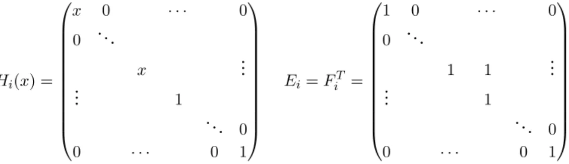
Ei, Fi and Hi. In the standard representation they have the following form
Hi(x) = x 0 · · · 0 0 . .. x ... .. . 1 . .. 0 0 · · · 0 1 Ei = FiT = 1 0 · · · 0 0 . .. 1 1 ... .. . 1 . .. 0 0 · · · 0 1
where the last line of Hi(x)with an x entry is the i-th line and the off-diagonal element
of Ei is the in the i-th line.
1.4.1 Thurston diagrams and cluster varieties associated to P GLn(C)
In the case of cluster manifolds associated to P GLn(C), the cluster seeds and tori can
be represented by Thurston diagrams on a strip by superimposing two wiring diagrams, one corresponding to positive simple roots, and the other corresponding to the negative ones. The Thurston diagram description has the advantage that both the evaluation map and the the Poisson structure are easily readable from it.
Figure 1.4 and Figure 1.5 show Thurston diagrams associated to generators of the braid semigroup. The diagram corresponding to a word whose length is longer than one is obtained by gluing the diagrams associated to the generators.
It is easy to verify that the seeds obtained from a Thurston diagram corresponding to a braid semigroup generator coincide with the ones defined in subsection 1.3.1 and that gluing Thurston diagrams corresponds to the amalgamation of the corresponding
1.5. bAnCluster X -manifolds
Figure 1.4: Thurston diagram corre-sponding to the generator si
Figure 1.5: Thurston diagram corre-sponding to the generator si
seeds. As mentioned above, the evaluation map is easily computable from a Thurston diagram corresponding to a braid semigroup element. See the following example.
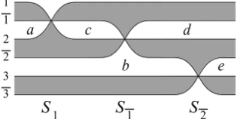
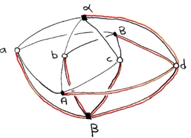
Example Let us consider the word s1s¯1s¯2in the braid semigroup of A3. The associated
Thurston diagram is depicted in Figure 1.6.
Figure 1.6: Thurston diagram associated to the word s1s¯1s¯2 in the braid semigroup of
A3.
The cluster variables are denoted by a, b, c and d. The evaluation map gives H1(a)H2(b)E1H1(c)F1F2H1(d)H2(e)
1.5
A
b
nCluster X -manifolds
The majority of the last section extends to the case of affine Dynkin diagrams. We present here the particular case of the ˆAtype following [FM14].
1.5.1 The coextended affine Weyl group
Let W be the type An Weyl group. The Weyl group W admits a central coextension
generator l with relations
sisi+1si= si+1sisi+1 for i = 1, ..., n
lsi= si+1l for i = 1, ..., n
sisj = sjsi for distant i, j = 1, ..., n
s2i = 1 for i = 1, ..., n
lN = 1
By analogy with the finite dimensional case, we introduce the braid semigroup related to W#. It is the semigroup freely generated by the simple roots of W# and their
opposites.
1.5.2 The Laurent realisation of the group [P GL#n(C)
In the Laurent realization, the group [P GL#n(C) can be identified with the group of expressions of the form M (λ)Tx where M (λ) is a Laurent polynomial valued n by n
matrix and Txis the operator acting by multiplicative shift by x that is
Tx1.M (λ)Tx2 = M (x1λ)Tx1x2
The loop group [P GL#n(C) has one more triple of generators in addition to those of P GLn which we denote E0, E0 and H0(x). In loop representation the matrices Ei for
i 6= 0, 0coincide with the corresponding matrices for finite-dimensional group P GLn
and the matrices Hi(x)get multiplied by Tx, i.e
Hi(x) = x 0 · · · 0 0 . .. x ... .. . 1 . .. 0 0 · · · 0 1 Tx, Ei= FiT = 1 0 · · · 0 0 . .. 1 1 ... .. . 1 . .. 0 0 · · · 0 1
for i > 0. For i = 0, we additionally have H0(x) = Txand
E0= 1 0 · · · 0 .. . . .. ... 0 . .. 0 λ · · · 0 1 F0 = 1 0 · · · λ−1 .. . . .. ... 0 . .. 0 0 · · · 0 1
1.5. bAnCluster X -manifolds
It is also useful to introduce the element Λ ∈ [P GLnhaving in the loop
representa-tion the form
Λ = 0 1 · · · 0 .. . . .. ... ... 0 · · · 0 1 λ · · · 0 0
This matrix has the property
EiΛ = ΛEi+1, FiΛ = ΛFi+1, Hi(x)Λ = ΛHi+1(x), i ∈ Z/N Z
i.e operator Λ acts as unit shift along the Dynkin diagram of [P GLn.
1.5.3 The Thurston diagram description
As in the An case, words in the braid semigroup of ˆAcan be represented by Thurston
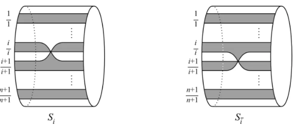
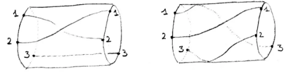
diagrams but, in that case, drawn on a cylinder instead of a strip. For i 6= 0 the Thurston diagrams are the same as in the non affine case, but viewed on a cylinder. These diagrams are shown in Figure 1.7 and Figure 1.8.
Figure 1.7: Thurston diagram correspond-ing to the generator si
Figure 1.8: Thurston diagram correspond-ing to the generator si
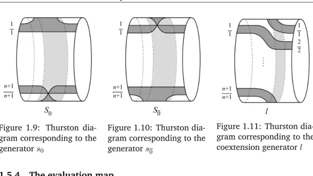
Thurston diagrams for the affine generators s0 and s0involve curves that are going
"behind" the cylinder and are shown in Figure 1.9 and Figure 1.10. The Thurston diagram associated to the coextension generator l is depicted in the Figure 1.11
The seeds associated to a word in the semigroup cWn freely generated by the si, si
for i ∈ Z/nZ and l can be determined by gluing the corresponding elementary Thurston diagrams and using the rule of the subsection 1.2.1.
Figure 1.9: Thurston dia-gram corresponding to the generator s0
Figure 1.10: Thurston dia-gram corresponding to the generator s0
Figure 1.11: Thurston dia-gram corresponding to the coextension generator l
1.5.4 The evaluation map
The definition of the evaluation map of subsection 1.3.3 does not apply directly in the coextended affine case because of the coextension generator l. As the generator l has no incidence on the cluster seed associated to a word, one way to circumvent the novelty is to use the relation
lsi = si+1l for i ∈ Z/nZ
to move all the occurrences of l to the end (or the beginning) of the word and then use the same rule as in the non affine case and finally multiply by the group element Λ to the correct power.
Chapter 2
Links and braids
2.1
Links
We recall notions of knot theory that will be needed later. We follow the exposition of [Tur12].
A link L ⊂ S3 is a finite set of disjoint circles embedded in S3. These circles are
called the components of L. If L is connected, it is called a knot. A link is polygonal if it is the union of a finite number of closed straight line segments. A link is tame if it is ambiently isotopic to a polygonal link. We only consider tame links. A link L ⊂ R3 ⊂ S3 is usually specified by a regular projection to a plane in R3. We fix
an orientation of S3. A link in S3 is ordered if its components are numbered. Let
L = L1∪ ... ∪ Ll ⊂ S3 be an ordered link. Let U =`li=1Ui be a regular neighborhood
of L and let E = S3\Int(U ) be the link exterior. Since E is a deformation retract of
S3\L, the group H1(E) = H1(S3\L) does not depend on the choice of U . We claim that
this group is canonically isomorphic to a free abelian group on l generators. Indeed, the exact homology sequence of the pair (S3, E)shows that
H1(E) = H2(S3, E) = l
L
i=1
H2(Ui, ∂Ui).
The regular neighborhood Uiof Lican be identified with a solid torus S1×D2where D2
is a closed 2-disc. Under the identification Ui = S1× D2the knot Li⊂ Ui corresponds
to the core S1\{pt} of S1×D2where pt ∈ IntD2. For any x ∈ S1, the 2-disc x×D2⊂ U i
meets Litransversally in one point. We orient D2so that the sign of this intersection is
+. The disc x × D2with this orientation is called a meridional disc in U
i. The oriented
loop x × ∂D2 ⊂ ∂U
i is called a meridian of Li. It is easy to see that the isotopy class
of the meridian on ∂Ui neither depends on the choice of x ∈ S1 nor on the choice of
identification Ui = S1× D2.
The exact homology sequence of the pair (Ui, ∂Ui)shows that H2(Ui, ∂Ui) = Z with
generator represented by a meridional disc of Li. Therefore H1(E) = Zt1⊕ ... ⊕ Ztl
Z[t±11 , ..., t ±1
l ]is the ring of Laurent polynomials in t1, ..., tl.
The group π1(E) = π1(S3\L) is called the group of L.
In this text we will only consider link diagrams that are connected, that is, we impose that the underlying four-valent graph is connected. Every link diagram can be transformed into a connected one with the help of the second Reidemeister move.
2.2
Milnor Torsion of link exteriors
In this section we recall the definition of the Milnor torsion of link exteriors and meth-ods of computation of this latter. We follow the exposition of [Tur12].
2.2.1 Torsion of chain complexes
Let C be a finite acyclic based chain complex of finite dimensional vector spaces over a field F. C = (0 → Cm ∂m−1 −−−→ Cm−1→ ... ∂1 −→ C1 ∂0 −→ C0 → 0)
Based means that, for each Ci, we have a distinguished basis ci.
Set Bi = Im(Ci+1 ∂i+1
−−−→ Ci) ⊂ Ci. Since C is acyclic, we have the following short exact
sequences:
0 → Bi ,→ Ci ∂i−1
−−−→ Bi−1→ 0
We choose, for each i, a basis bi of Bi. By the exactness of the previous sequence, we
can complete the basis bi to a basis of Ci by lifting elements of the basis bi−1. We set
bibi−1= (b1i, ..., bik, eb1i−1, ..., ebli−1)
where the ebji−1are lifts of the bji−1 to Ci and k and l are the dimension of Bi and Bi−1
respectively. Let P = (pij)be the transition matrix from the basis cito the basis bibi−1.
We write
[bibi−1/ci] = det(P )
We are now ready to define the torsion of C.
Definition The torsion of C is
τ (C) =
m
Q
i=0
[bibi−1/ci] ∈ F∗
Remark – The torsion depends on the distinguished basis ci but not on the choice of
the bi.
Computation of the torsion with the method of matrix τ -chains
2.2. Milnor Torsion of link exteriors C = (0 → Cm ∂m−1 −−−→ Cm−1 → ... ∂1 −→ C1 ∂0 −→ C0 → 0) Let Ai be the matrix of the chain homomorphism ∂i: Ci+1→ Ci
Ai = (aijk) j=1,...,dimCi
k=1,...,dimCi+1
Definition A matrix chain for C is a collection of sets α = (α0, α1, ..., αm), where
αi⊂ {1, 2, ..., dimCi}, so that α0= ∅. We think of αi as a set of basis vectors of Ci.
Let Si = Si(α)be the submatrix of Ai formed by the entries aijk with k ∈ αi+1and
j /∈ αi. The matrix chain α is called a τ -chain if S0, S1, ..., Sm−1 are square matrices.
The τ -chain α is said to be non-degenerate if det Si 6= 0 for all i.
Proposition 2.1 Let α = (α0, α1, ..., αm)be a non-degenerate τ -chain for C. Then
τ (C) = ± m−1 Q i=1 (det Si(α))(−1) i+1
Computation of the torsion with the method of chain contractions
The chain contraction method for the computation of the torsion could be more rele-vant for a cluster theoretic interpretation of our construction. Indeed, in that setting, we can express the torsion as the determinant of an operator from black vertices to white vertices, or the opposite. The only step missing is an appropriate embedding of our graph in a surface so that we could express the torsion as the dimer partition function.
2.2.2 Milnor torsion of link exteriors
Let X be a finite connected CW-complex. Fix x0 in X and let π = π1(X, x0) and
H = H1(X; Z) and G = H/TorsH. Let p : ¯X → X be the covering of X corresponding
to the morphism π → G this covering is called the maximal free abelian covering of X. We endow ¯Xwith the CW-structure induced from X. We orient all open cells of X and orient the cells of ¯X in such a way that the restriction of p to each cell is orientation preserving. The action of H on ¯X by covering transformations induces an action of G on the cellular chain groups Ck( ¯X). Extend this action linearly to an action of Z[G].
In this way, Ck( ¯X) becomes a Z[G]-module. Note that the boundary homomorphism
∂ : Ck( ¯X) → Ck−1( ¯X)is linear over Z[G] for all k ≥ 1. Let {eki} be the set of oriented
k-cells of X ordered in an arbitrary way. Choose over each ek
i a k-cell ¯eki in ¯X. Then
the set {¯eki} is a basis of Ck( ¯X), i.e.,
Ck( ¯X) =
L
i
Z[G]¯eki.
Thus, C( ¯X) is a free and based chain complex over Z[G]. Let Q(G) be the quotient field of Z[G]. Let us consider the following chain complex :
C = Q(G) N
Z[G]
C( ¯X)
Definition If H?(C) = 0then the Milnor torsion of X is the torsion τµ(X) = τ (C) ∈
Q(G)/ ± G.
Definition The fundamental groupoid of a topological space X is a category whose
objects are the points of X and whose morphisms are endpoint-preserving homotopy classes of paths in X.
Definition A local coefficients system on X is a functor from the fundamental groupoid
of X to the category of abelian groups.
Every morphism π1(X, x0) → Gof the fundamental group of X to an abelian group
gives rise to an isomorphism class of a local coefficient system whose fiber is isomorphic to Z[G], the group ring of G.
Definition The Milnor torsion of a link exterior is the torsion of the relative cellular
chain complex of (X, ∂X) in a local coefficients system induced by the abelianization morphism π → H → Q(H).
2.3
Braids
2.3.1 The Artin braid groups
In this subsection we recall the different definitions of the braid groups. We mainly follow [KT08].
Algebraic definition
We give an algebraic definition of the braid group Bn for n a positive integer,
formu-lated in terms of a group presentation by generators and relations.
Definition The Artin braid group Bn is the group generated by n − 1 generators
σ1, σ2, . . . , σn−1 subject to the relations
σiσj = σjσi for all i, j = 1, 2, . . . , n − 1 with |i − j| ≥ 2
σiσi+1σi = σi+1σiσi+1 for all i = 1, 2, . . . , n − 2
Remark – This presentation can be recovered from the An−1 Dynkin diagram
Let β ∈ Bn, let us define an algebraic representative of β to be an element of F2(n−1)
2.3. Braids
Geometric braids
We give the geometric definition of the braid groups. By a topological interval we mean a topological space homeomorphic to the closed interval [0, 1]. We denote by D2 the
open unit disc in R2.
Definition A geometric braid on n strings is a subset β of [0, 1]×R2formed by n disjoint
topological intervals called the strings of β such that the projection [0, 1] × R2 → [0, 1]
maps each string homeomorphically onto [0, 1] and
β ∩ ({0} × R2) = {(0, 0, 1), (0, 0, 2), . . . , (0, 0, n)} β ∩ ({1} × R2) = {(1, 0, 1), (1, 0, 2), . . . , (1, 0, n)} A braid on n strings is an isotopy class of geometric braids.
Given two geometric braids on n strings β1, β2 ⊂ [0, 1] × D2, we define their product
β1β2 to be the set of points (t, x, y) ∈ [0, 1] × R2 such that (2t, x, y) ∈ β1 if 0 ≤ t ≤
1/2 and (2t − 1, x, y) ∈ β2 if 1/2 ≤ t ≤ 1. The formula (β1, β2) 7→ β1β2 defines a
multiplication on the set of braids on n strings.
Braid diagrams
We will give a definition of braid diagram slightly stronger than usual in order to have a bijective correspondence between braid diagrams on n strands and algebraic repre-sentatives of elements of the braid group Bn.
A braid diagram on n strands is a set D ⊂ [0, 1] × R split as a union of n topological intervals called the strands of D such that the following conditions are met:
1. The projection [0, 1] × R → [0, 1] maps each strand homeomorphically onto [0, 1] 2. Every point of {0, 1} × {1, 2, . . . , n} is the endpoint of a unique strand.
3. Every point of [0, 1]×R belongs to two strands at most . At each intersection point of two strands, these strands meet transversally and one of them is distinguished and said to be undergoing, the other strand being overgoing.
4. The projection [0, 1]×R → [0, 1] maps each intersection points to a different point of [0, 1].
Remark – The usual definition of a braid diagram is a set D as above satisfying only
the first three conditions.
We can consider braid diagrams as a special case of graphs with additional structure describing the nature of the crossings. We call half-arc of a braid diagram an edge of the underlying graph. There are two types of half arcs. Terminal half arcs corresponding to an edge of the underlying graph having a univalent vertex and inner half arcs whose underlying edge connects two four-valent vertices.
2.3.2 Colored oriented braids groupoid
A colored oriented braid on n strings is a braid on n strings called the underlying braid with the additional data of a function which assigns an orientation and an integer for each string. Diagrammatically, a colored braid is a classical braid with a labeling of each strand with an integer and an arrow indicating the orientation. Multiplication is allowed if the labellings and orientations coincide.
Weighted braid diagrams
We will call weighted braid diagram a braid diagram in the sense of the previous defi-nition with the assignment of a variable for each half-arc of the diagram.
2.3.3 Annular braid group
Geometric definition
Annular braids can be defined in a way similar to the classical braids. Let A be an
annulus,A = S1× [−1, 1], a geometric annular braid on n strands is a set β ⊂ A × I
formed by n disjoint topological intervals called the strands of β such that each strand is mapped homeomorphically onto I by the projectionA × I → I and
β ∩ (A × {0}) = {(e2ikπn , 0, 0) ; k = 0, 1, ..., n − 1}
β ∩ (A × {1}) = {(e2ikπn , 0, 1) ; k = 0, 1, ..., n − 1}
Examples of geometric annular braids are shown in Figure 2.1. An annular braid is an isotopy class of geometric annular braids. Composition of annular braids is defined by gluing the thickened cylinders, respecting the S1coordinates.
Figure 2.1: Examples of annular braids. On the left, the generator σ1 and on the right
τ−1
Algebraic definition
2.4. Burau representations
σ1, ..., σn, τ
and is ubject to the relations
σiσj = σjσi for distant i, j = 1, ..., n
σiσi+1σi= σi+1σiσi for i ∈ Z/nZ
σiτ = τ σi+1 for i ∈ Z/nZ
This presentation coincides with the presentation of the coextended affine type A braid group obtained from the type bADynkin diagram. The latter is a necklace with n nodes and the coextension generator ρ is the automorphism of diagram which rotates it by an angle of 2πn. From now on we will denote by B#
b
An−1 the annular braid group.
This group injects into the braid group on n + 1 strands. Indeed, the annular braid group on n strands B#
b An−1
is isomorphic to Dn+1 which is the subgroup of the classical
braid group on n + 1 strands for which the strand beginning in position one also ends in position one. The first strand in the Dn+1 picture corresponds to the core of the
cylinder in the annular picture. For the demonstration that these group coincide (and coincide with the braid group of type Bn) we refer to the paper of Kent and Peifer
[KIP02]. The Dn+1 point of view is convenient to define the Burau representation of
annular braids.
2.3.4 Colored oriented annular braids groupoid
A colored oriented annular braid on n strands is an annular braid with the additional choice for each strand of a color, that is an integer between 1 and n, and an orientation, or equivalently a sign. Composition of colored oriented annular braids is allowed if the colors and orientation coincide. The inverse of a colored oriented annular braid is given by the inverse of the underlying annular braid with the same coloring and orientations. This endows the colored oriented braids on n strands with the structure of a groupoid.
2.4
Burau representations
2.4.1 The Burau representations of colored oriented Artin braids
The reduced Burau representation
Let T be a colored oriented braid on n strands and N (T ) an open tubular neighborhood of T in the cylinder D2× [0, 1], we denote by X the exterior of T .
X := (D2× [0, 1]) − N (T )
Let lk(c, c0)be the linking number of the curves c and c0. We denote by cl(s) the closure of the strand s and by Si the set of the strands of T colored with i
Si := {strands of T colored with i}
Let π1(X) be the fundamental group of X and φ the morphism from π1(X) which
counts the total linking number of a closed curve around (the closure of) the strands marked with the same color.
φ : π1(X) → Q(t1, u1, ..., tn, un) [γ] 7→ n Y i=1 (tiui)ki where ki:= X s∈Si
lk(γ, cl(s)). The application φ induces an isomorphism class L of local coefficients system on X.
Let D0 := X ∩ (D2× {0}) and D1 := X ∩ (D2× {1}). We denote by L0 and L1the
induced local coefficients systems on D0and D1 respectively. We define X01:= (∂D2×
[0, 1] ∪ N (T )). The inclusions i0: (D0, ∂D0) → (X, X01)and i1 : (D1, ∂D1) → (X, X01)
are homotopy equivalences and thus induce isomorphisms in homology. H1(D0, ∂D0; L0)
(io)∗
−−−→ H1(X, X01; L) (i1)∗
←−−− H1(D1, ∂D1; L1)
Definition We define the reduced Burau representation of colored oriented braids as
Chapter 3
Cluster manifolds associated to
links, braids and their invariants
3.1
Dimer model for the torsion of link exteriors
3.1.1 Introduction
We reinterpret and extend the dimer model for the Alexander polynomial of knots of Cohen, Dasbach and Russel [CDR14] to the Milnor torsion of link exteriors.
Let L =Sn
i=1Ki be a colored oriented link in S3 and X := S3− N (L) its exterior.
We denote by DL an arbitrary connected diagram of L, that is a regular projection of
L on S2 such that the underlying quadrivalent graph is connected. We construct an
application
DL7→ (Γ i
− → X)
which assigns to DL a bipartite graph Γ embedded in X. The graph Γ can be viewed
as a subgraph of the 1-skeleton of the first barycentric subdivision SC of a cellular decomposition C of (X, ∂X) naturally constructed from the diagram DL. The vertices
of Γ are the barycenters of the cells of C. The edges of Γ are the 1-cells of SC which connect the barycenters of the cells of C. The bipartition of the set of vertices of Γ comes from the parity of the dimension of the cells of C.
The bipartite graph constructed by Cohen, Dasbach and Russel is the subgraph of Γ corresponding to the 2-skeleton of the cellular decomposition.
Let φ be the abelianization morphism of the fundamental group of X π1(X) φ −→ Zn γ 7→ n Y i=1 tki i
where ki denotes the linking number of the loop γ with the component Ki of L. The
image of φ by the morphism induced in cohomology by the graph embedding i gives an element
i∗(φ) ∈ H1(Γ; Q(t1, . . . , tn))
We compute the Milnor torsion of X from Γ and i∗(φ). Let L be a local coefficients system on X induced by φ. The Milnor torsion of X is the torsion of the acyclic chain complex (C∗(C; L), ∂∗). We have
C∗(C; L) ' C0(Γ; Q(t1, . . . , tn))
and the differential ∂∗ is determined by a lift of i∗(φ)to C1(Γ; Q(t1, . . . , tn)).
The computation of the torsion from this data by the method of τ -chains [Tur86] extends the dimer model for the Alexander polynomial of [CDR14] in the following sense : the algorithm of Cohen, Dasbach and Russel consists, from our point of view, in a particular choice of lift of i∗(φ)and a particular choice of τ -chain.
The computation by the method of chain contractions [Coh73] enables to express the torsion of X as a dimer partition function.
3.1.2 A CW-complex structure on a link complement
Starting from a regular projection of a link, we endow the link exterior with the strucure of a CW-complex. We will simultaneously construct the CW-complex structure on the interior and the boundary of X, however the cell structure on the latter is not important since we will mod the boundary out in our computations. The 1-skeleton of the CW-complex structure on the link exterior and part of the image of the attaching map of a 2-cell corresponding to a region of the diagram are depicted in Figure 3.1.
Figure 3.1: The 1-skeleton of the CW-complex structure on the link exterior and part of the image of the attaching map of a 2-cell corresponding to a region of the diagram
3.1. Dimer model for the torsion of link exteriors
0-cells
We consider eight 0-cells for each crossing of the diagram as can be seen in the Fig-ure 3.1. All of the 0-cells are on the boundary of X. The 0-cells are depicted in red in figure 3.1.
1-cells
Each crossing gives eight 1-cells on ∂X. We add 4n 1-cells on ∂X, where n stands for the half arcs of the link diagram, that is, the number of edges of the underlying four-valent graph. In the interior of X, for each crossing of the link diagram we add a vertical 1-cell joining the torus under the projection plane and the torus above it and we orient them upwards. The 1-cells of our decomposition of ∂X are depicted in orange, and the 1-cells which belong to the interior are depicted in green in Figure 3.1.
2-cells
We complete the cellular decomposition of ∂X, which is a union of tori, for that we need four 2-cells per half-arc of the link diagram. In the interior of X we glue a 2-cell for each region of the link diagram (that is each complementary region in the plane of the quadrivalent graph corresponding to the link projection). We glue them in each region following the boundary of the link exterior and following our previously added 1-cells at the crossings. In Figure 3.1 a part of the image of the attaching map of a 2-cell corresponding to a region of the diagram is depicted in blue.
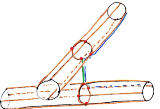
3-cells
We eventually need to glue two 3-cells, one under the projection plane and one over. Attaching maps of the 3-cells near a crossing are described in the Figure 3.2.
3.1.3 Graph encoding the cellular structure
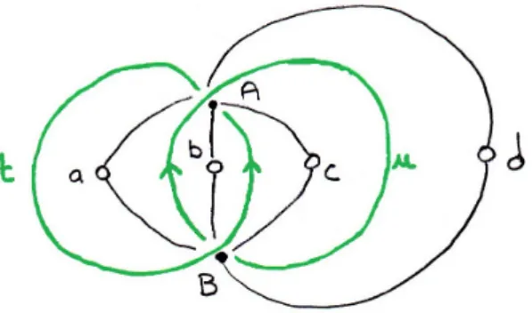
Figure 3.3: Link diagram and associated bipartite graph encoding the 2-skeleton of the relative cellular structure.
Figure 3.4: Bipartite graph associated to a link diagram.
In this subsection we will construct a bipartite graph encoding the CW-complex structure on the link exterior modulo its boundary (X, ∂X) described above. The Hopf Link will serve as an example. We start with an oriented and ordered link diagram. Recall that we impose that the diagram is connected.
Black vertices
We put a (round) black vertex for each 1-cell of our cellular decomposition, that is at crossings of the link diagram. And (square) black vertices for the 3-cells.
White vertices
We put a white vertex for each region of the diagram, that is, for each connected component of the complementary in the plan of projection of the underlying four-valent graph.
3.1. Dimer model for the torsion of link exteriors
Edges
We put an edge between a white vertex and a black vertex if the corresponding crossing and region are adjacent. Edges are oriented from white to black vertices.
From this point of view. The bipartite graph constructed by Cohen, Dasbach and Russel is the subgraph corresponding to the 2-skeleton of the cellular decomposition of the link exterior relative to its boundary. See Figure 3.3 for the subgraph and Figure 3.4 for the complete graph, both in the case of the usual Hopf link diagram.
3.1.4 Weighting on the graph
We will assign weights to edges of our graph Γ with values in the free abelian group generated by t1, ..., tl, that is the weighting may be viewed as an element of C1(Γ, Zl).
The weighting on Γ is induced by the embedding Γ ⊂ E. Consider the cellular cochain complex of Γ with coefficients in Zl.
0 → C0(Γ, Zl)−→ Cδ 1(Γ, Zl) → 0
We have H1(Γ, Zl) = C1(Γ, Zl)/δC0(Γ, Zl) and by the universal coefficient theorem
H1(Γ, Zl) =Hom(H1(Γ, Zl)). The weighting we are interested in is a lift to C1(Γ, Zl)
of the cocycle of H1(Γ, Zl)iduced by the inclusion Γ−→ E.i
H1(Γ)−i→ H∗ 1(E) ' Zl
c 7→ tlk(c,L1)
1 ...t lk(c,Ll)
l
Suppose our link has n components, we assign a variable t1, t2, ..., tnto each
com-ponent. In our example, in Figure 3.3, these variables are t and u. Now we will put weights on our graph. These weights will encode a local coefficients system induced by the abelianization morphism from the fundamental group of the link to the free abelian group on n generators :
ρ : π1(X) → ht1, t2, ..., tni
γ 7→lk(L, γ)
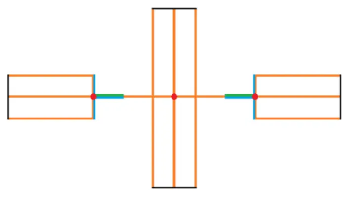
It can also be interpreted as a choice of a lift of each cell of our cellular decomposi-tion of the link exterior in the maximal abelian cover of this latter. We orient our graph from white vertices to black vertices. We want to weight the graph so that the product of the weights along an oriented cycle c, where we take the inverse of the edge variable if we travel along the edge against its orientation, to be equal to its homology class, lk(c, K). To do so, we can choose a maximal tree in our graph, as in Figure 3.5 where the maximal tree is depicted in orange, we assign the weight 1 to all the edges of the
maximal tree and label the remaining edges with the weight satisfying the preceding rule. We illustrate this in the example in Figure 3.6 and Figure Figure 3.7.
Figure 3.5: A maximal tree in the bipartite graph.
We have splitted the graph in two as it turns out that they will correspond respec-tively to ∂1 and ∂2 in the cellular chain complex C∗(X, ∂X; E) of the link exterior
modulo its boundary in a local coefficients system E determined by ρ. In these figures, orange edges correspond to the maximal tree, green variables correspond to the homol-ogy class of the cycles corresponding to the faces in which they are and blue variables are the weights assigned to the edges so that our rule is followed.
Figure 3.6: Weights corresponding to ∂1
Figure 3.7: Weights corresponding to ∂2
3.1.5 Computation of the torsion of the link exterior
We present here two methods of computation of the torsion of a link exterior from the weighted bipartite graph previously constructed. The first one is the method of τ-chains and the second one, the method of chains contractions. The τ -chain point of view is useful to understand of the transition from links to braids, whereas the chain contraction point of view is best suited for a cluster theoretic of the torsion of link
3.2. Burau cluster submanifolds associated to braids exteriors as this latter can be expressed as a dimer partition function. τ-chains
We have the following cellular chain complex C = C∗(X, ∂X; E) of the link exterior
modulo its boundary with a local coefficients system determined by the abelianization morphism. C = (0 → C3 ∂2 −→ C2 ∂1 −→ C1→ 0)
We can determine the matrices Ai of the ∂i from the bipartite graph. In our example,
in the basis {α, β} of C3, {a, b, c, d} of C2and {A, B} of C1, the matrices are given by :
A2 = t−1 1 t−1u 1 u 1 1 1 A1 = −t t −1 1 −1 u−1 −u−1 1 !
Now let us consider the τ -chain α = (α3, α2, α1)where α3= {α, β} α2= {b, d}and
α1= {∅}. With this τ -chain we have :
S2(α) = t−1 1 u 1 ! S1(α) = t 1 u−1 1 !
3.2
Burau cluster submanifolds associated to braids
In this section, we associate to colored oriented braid representatives, pairs consisting of a cluster X -manifold related to the type An braid semigroup and a submanifold of
the latter.
More precisely, we construct two maps ψr and ψu, the first one from the set of
rep-resentatives of colored oriented braids on n strands, Brc
n, to the set of pairs {(MAn, S)}
consisting of an An type cluster X -manifold and a submanifold of it. And the
sec-ond one from Brc
n to the set of pairs {(MAn−1, S)}consisting of an An−1 type cluster
X -manifold and a submanifold of it. Brcn ψ r −→ {(XAn− manifold, submanifold)} (3.1) Brcn ψ u −−→ {(XAn−1− manifold, submanifold)} (3.2)
The map ψr can be viewed as a translation in the context of braids of the
construc-tion in secconstruc-tion 3.1.
By construction, these maps respect the multiplications in the sense that, to a prod-uct of colored braid representatives corresponds the multiplication of the associated cluster manifolds and its restriction to the submanifolds.
The composition of these maps with the evaluation map restricted to the submani-folds is independent of the chosen representatives and gives projective versions of the generalized reduced and unreduced Burau representations respectively.
In subsection 3.2.1 we construct the map ψrand prove the following theorem.
Theorem 3.1 For n ≥ 3, let ρ : Bc
n → GLn+1(Q(t1, u1, . . . , tn, un))be the composition
of the map r, which assigns an arbitrary representative to colored oriented braid, with ψr
and the evaluation map restricted to the second factor :
ρ : Bnc −→ Brr c n
ψr
−→ {(MAn, S)}−−→ GLev|S n+1(Q(t1, u1, . . . , tn, un))
The map ρ is a representation of the colored oriented braid groupoid on n strands, which coincides with the generalized reduced Burau representation.
In subsection 3.2.3 we construct the map ψu and prove the corresponding theorem.
Theorem 3.2 For n ≥ 3, let ρu : Bnc → P GLn(Q(t1, . . . , tn))be the composition of the
map r, which assigns an arbitrary representative to colored oriented braid, with ψu and the evaluation map restricted to the second factor :
ρu : Bcn r − → Brc n ψu −−→ {(MAn−1, S)}−−→ P GLev|S n(Q(t1, . . . , tn))
The map ρu is a projective representation of the colored oriented braid groupoid on n
strands, which coincides with the projectivization of the generalized unreduced Burau rep-resentation.
3.2.1 Burau cluster submanifolds associated to oriented colored braids, the reduced case
We construct the map ψr from the set of representatives of colored oriented braids
on n strands to the set of pairs consisting of an An type cluster X -manifold and a
submanifold of it.
Brnc ψ
r
−→ {(XAn− manifold, submanifold)}
First, we define the ambient cluster X -manifold. Algebraically by assigning to an alge-braic representative of the underlying braid, an element of the braid semigroup; and diagrammatically by associating a Thurston diagram to a diagrammatic braid represen-tative. Then we give the rule of construction of the submanifolds. In the reduced case, this rule is a translation, in the context of braids, of the construction in section 3.1.
3.2. Burau cluster submanifolds associated to braids
Construction of the ambient manifold
Let βr
c be a colored oriented braid representative on n strands and βr ∈ Bnthe
under-lying braid representative. We associate to βran element of W
nwith the morphism of
semigroups ψ defined below.
ψ : F2(n−1)→ Wn σi7→ sisi+1
σi−17→ si+1si Recall from section 1.1 that to the element ψ(βr)of W
ncorresponds a seed, XJ(ψ(βr)),
of the Ancluster X -manifold associated to p(ψ(βr)) ∈ B. Diagramatically the
construc-tion of the manifolds for the braid representatives semigoup generators translates in Figure 3.8 and Figure 3.9.
Figure 3.8: Diagrammatic rule for the construction of the ambient variety
Figure 3.9: Diagrammatic rule for the construction of the ambient variety The Thurston diagram corresponding to a braid diagram with more than one cross-ing is obtained by glucross-ing the diagrams associated to the generators of Bn and their
inverses.
Remark – In the particular seed tori of the cluster manifolds we have constructed the
cluster variables correspond to half arcs of the underlying braid representative.
Construction of the submanifold
We construct in the particular seed associated to ψ(βr) a submanifold. As mentioned
above, in that particular seed, the cluster variables correspond to half arcs of the braid diagram. The rule of construction of the submanifold is reminiscent of the construction of section 3.1. The parametrization for the submanifolds is described in Figure 3.10 and Figure 3.11.