Buoyant jet behavior in confined regions

BUOYANT JET BEHAVIOR IN CONFINED REGIONS by

David J. Fry and E. Eric Adams

Energy Laboratory Report No. MIT-EL 81-050 September 1981

COO-4683-9

BUOYANT JET BEHAVIOR IN CONFINED REGIONS

by David J. Fry and E. Eric Adams Energy Laboratory and

Ralph M. Parsons Laboratory for

Water Resources and Hydrodynamics Department of Civil Engineering Massachusetts Institute of Technology

Cambridge, Mass. 02139

Prepared under the support of Division of Central Solar Technology

U.S. Department of Energy Under Contract No. ET-78-S-02-4683

Energy Laboratory Report No. MIT-EL 81-050

ABSTRACT

Previous confined jet studies have emphasized the behavior of

non-buoyant jets inside ducts or near plane boundaries (Coanda effect). Buoyancy, however, is a major factor in the confined jet behavior

experienced in many environmental fluid mechanics problems and, in

particular, in the external fluid mechanics associated with an operating Ocean Thermal Energy Conversion (OTEC) plant. In many of these cases confinement and buoyancy offer opposing influences on jet trajectory and diffusion.

An experimental set-up was designed, similar to some encountered in OTEC, but simple enough to facilitate accurate measurements and to allow the results to be interpreted through dimensional analysis. The particular experimental situation chosen was a submerged, negatively buoyant, horizontal, radial jet discharging into ambient water which was initially uniform in temperature and density. A near-surface intake was included in some experiments and not in others. Two distinct flow regimes were possible depending on the relative importance of buoyancy and confinement.

The first flow regime (buoyancy-dominated) is termed a detached

jet. The ambient region above the jet is an irrotational flow consisting entirely of original ambient fluid. The flow magnitude is determined by the entrainment requirements of the upper boundary of the jet and the intake flow, if any. The ambient region below the jet is made up of fluid pulled from the jet as it nears a vertical trajectory. The flow here is rotational and at a lower temperature than the original ambient

fluid.

The second flow regime (confinement-dominated) is termed an attached jet. Low pressures in the circulating region above the jet pull the jet to the surface. After impact the jet flow splits and no

longer can be characterized as a jet. The portion of jet flow downstream from the impact point is negatively buoyant with respect to the original ambient fluid and therefore sinks - some returning as entrainment for the underside of the jet. In this case neither the top nor the bottom ambient region has the temperature of the original ambient water.

Seventeen experiments yielded temperature and trajectory data

on the radial jet in both of the flow regimes. Velocity data also were collected in the upper ambient region for the detached jet. Finally discharge conditions that caused transition from one flow regime to the other were determined. A hysterisis effect was noted as the conditions for "attaching" a detached jet were different from those needed to "detach" an attached jet.

Dimensional analysis yielded a single dimensionless number that

was fairly successful at predicting the transition points between regimes. However, three dimensionless numbers were apparently needed to completely characterize the experimental behavior. The dimensional analysis was also helpful in formulating an analytical jet model.

An integral jet model (based on a spreading assumption) was

successfully adapted to include effects of velocity and pressure fields in ambient regions. The model predicts jet trajectories, velocities, and temperatures, and transitions of experiments between flow regimes.

The model can be applied to plane jets as well and buoyant and non-buoyant confined plane jet data from other studies were also compared with model predictions.

ACKNOWLEDGEMENTS

This report represents the Ph.D. Thesis of the first author presented to the Department of Civil Engineering, MIT. The work was sponsored by the U.S. Department of Energy, Division of Central Solar Technology, under Contract No. ET-78-S-02-4683. The contract was managed through the Water Resources Program at Argonne National Laboratory. The cooperation of Dr. Lloyd Lewis at DOE and of Drs. Jack Ditmars and Robert Paddock at ANL is appreciated. Dr. Paddock's detailed written comments on the draft copy of the report were particularly helpful.

I am greated indebted to the patience and guidance of my thesis advisor Dr. E. Eric Adams. A lot of the work he unselfishly assumed in M.I.T.'s

OTEC project was aimed at freeing me to work on this thesis. My work benefited greatly from his constant availability for long discussions and the encourage-ment provided by his genuine interest in the ongoing experiencourage-ments. The

dimensional analysis of the thesis problem in particular is mainly a result of his insights.

The long, late hours contributed during the experiments by graduate research assistant Mr. David Coxe are greatly appreciated. His ideas and remarkable ability to get things done were valuable assets in the OTEC project work we did together.

Special thanks go to Mrs. Zigrida Garnis for the excellent typing of this thesis, especially the long tables. On the few occasions when

time was a factor, her unsolicited willingness to stay till the job was done was gratefully acknowledged.

Several professors at the R.M. Parsons Laboratory contributed to this work in discussions. Special thanks are expressed to the members of my thesis committee, Professor Donald R.F. Harleman and Professor Keith Stolzenbach, who at several points reviewed the progress of this work and offered valuable suggestions and insights. Also the "off" hours spent here with laboratory students and personnel were essential in

providing the balance and perspective needed to sustain academic and research efforts.

I also wish to thank Mr. Edward McCaffrey and Mr. Roy Milley who kept everything electronic and otherwise in the lab working. The friendships, developed over many equipment problems and lunch hours in the shop, were an enjoyable part of my years at MIT. The fine craftmanship displayed in the OTEC experimental model is due to the care and skill of MIT machinist Arthur Rudolph.

I wish to thank my parents and brothers for their continuous support and interest in my work. Their willingness to understand the details of it resulted in valuable suggestions.

Finally and foremost I wish to thank my wife Valthea. Her patience, understanding, and sacrifice were contributed unselfishly so that I could finish my work at MIT the way I wanted to.

Table of Contents Page Abstract 2 Acknowledgements 4 Table of Contents 5 I. Introduction 10

1.1 Occurrence of Confined Jets 10

1.2 OTEC Operation 13

1.3 OTEC and Confined Jets 16

1.4 Objectives of this Study 16

1.5 Summary of the Study 19

II. Results of Related Investigations 22

2.1 The Turbulent Jet 22

2.2 Experimental Determination of Jet Behavior 25

2.3 Integral Jet Models 28

2.3.1 Closure Problem 29

2.3.2 Buoyancy 30

2.3.3 Boundaries 30

2.4 Review of Basic Jet Investigations 32

2.4.1 Unconfined Non-Buoyant Jets 33

2.4.1.1 Parameterization 33

2.4.1.2 Profile Data 33

2.4.1.3 Closure Relation Data 36

2.4.1.4 Radial Jet Behavior 39

2.4.2 Zone of Flow Establishment 39

2.4.2.1 Parameterization 40

2.4.2.2 Profile Data 40

2.4.2.3 Spreading Relation 42

2.4.2.4 Radial Jet Behavior 42

2.4.3 Co-flowing Ambient Fluids 46

2.4.3.1 Parameterization 46

2.4.3.2 Profile Data 46

2.4.3.3 Spreading Relation 48

Page

2.4.4 Counter-flowing Ambient Fluids 51

2.4.4.1 Parameterization 51

2.4.4.2 Profile Data 51

2.4.4.3 Spreading Relation 51

2.4.4.4 Radial Jet Behavior 56

2.4.5 Buoyant Unconfined Jets 56

2.4.5.1 Parameterization 56

2.4.5.2 Profile Data 58

2.4.5.3 Spreading Relation 58

2.4.5.4 Radial Jet Behavior 60

2.4.6 Symmetry in Deflected Plane Jets 60

2.4.6.1 Radial Jet Behavior 62

2.5 Other Confined Jet Studies 64

2.5.1 Ducted Jets 64

2.5.2 Offset Plane Boundaries 66

2.5.3 Angled Plane Boundaries 70

2.6 Summary 72

III. Theoretical Considerations 75

3.1 Experimental Determination of Flow Field 75

3.1.1 Flow Rate Length Scale - 1i 78

3.1.2 Buoyancy Flux Length ScaleQ- iB 81

3.1.3 Confinement Length Scale - 1H 82

3.1.4 Radial Length Scale - 1 82

r

3.1.5 Conclusions 82

3.2 Integral Jet Model - Jet Equations 84

3.2.1 Coordinate System 85

3.2.2 Basic Equations 87

3.2.3 Steady, Turbulent Flow Equations 90

3.2.4 Scale Variables 92

3.2.5 Jet Structure 94

3.2.6 Conservation Equations of the Integral Jet Model 99

3.2.7 Additional Jet Equations 101

3.3 Integral Jet Model - Ambient Region Equations 103 3.3.1 Ambient Region with a Remote Boundary 103 3.3.2 Ambient Region with an Impacted Boundary 105

3.3.2.1 Coherent Impacted Boundary 106

3.3.2.2 Diffuse Impacted Boundary 108

---Page

3.4 Integral Jet Model Solution Method 112

3.4.1 General ₁₁₂

3.4.2 Flow Regime Limits with the Integral Jet Model 114

3.4.2.1 Detached Jet Limits 115

3.4.2.2 Attached Jet Limits 116

IV. Physical Experiments ₁₁₇

4.1 Experimental Layouts 117

4.1.1 Model Basin 117

4.1.2 Experimental Model 117

4.1.3 Flow Circuits ₁₁₇

4.2 Measurement Systems 120

4.2.1 Temperature Measurement System 120

4.2.1.1 Equipment 120 4.2.1.2 Calibrations 122 4.2.1.3 Data Reduction ₁₂₃ 4.2.2 Trajectory Photographs 125 4.2.2.1 Equipment ₁₂₅ 4.2.2.2 Calibrations 125 4.2.2.3 Data Reduction 125

4.2.3 Hydrogen Bubble Velocity Photographs 127

4.2.3.1 Equipment ₁₂₇ 4.2.3.2 Calibrations ₁₂₈ 4.2.3.3 Data Reduction 128 4.3 Experiments ₁₃₀ 4.3.1 Experimental Parameters 130 4.3.2 Experimental Procedure ₁₃₀

V. Analytical Predictions of Experimental Results 134

5.1 Preliminaries ₁₃₄

5.1.1 Pressure and Temperature Below a Detached Jet 134 5.1.2 Temperature below an Attached Jet 136 5.1.3 Impact Momentum Balance for an Attached Jet 137 5.1.4 Comparisons with Dimensionless Numbers 137

5.2 Flow Regime Limits 140

Page

5.3 Jet Behavior 147

5.4 Integral Jet Model Sensitivities 158

5.4.1 Detached Jet Sensitivities 158

5.4.2 Attached Jet Sensitivities 159

VI. Comparison of Integral Jet Model with Other Sources of Data 162

6.1 Ducted Plane Jets 162

6.2 Plane Jets with an Offset Plane Boundary 164

6.2.1 Non-Buoyant Jet Cases 164

6.2.2 Buoyant Jet Cases 166

6.2.2.1 Complementary Buoyancy and Confinement

Effects 166

6.2.2.2 Opposing Buoyancy and Confinement

Effects 169

6.3 Plane Jets with Angled Plane Boundaries 172 VII. Applications to OTEC Plant Operation 177 7.1 Example Application to a 100 MW OTEC Plant 177 7.1.1 Evaporator Discharge Recirculation 177

7.1.2 Mixed Discharge Recirculation 181

7.1.3 External Plant Mixing of Evaporator and

Condenser Discharges 181

7.2 Integral Jet Model Extensions for Ambient

Stratification 183

7.2.1 Neutral Buoyancy Levels 184

7.2.2 Jet Spreading 187

7.2.3 Extent of Ambient Flow Fields 187

7.2.4 Diffuse Impacted Boundaries 189

7.3 Separate Ports 189

7.4 Non-Horizontal Discharges 190

7.5 Ambient Currents 190

VIII. Summary and Conclusions 194

8.1 Motivation 194

8.2 Summary 195

8.3 Important Results and Conclusions 196

Bibliography 198

Page Appendix I _{Dimensional Comparison of Experiments and the Integral}

Jet Model 207

Appendix II Integral Jet Model Sensitivities ₂₂₅

Appendix III 3-D Plots of Flow Transition Surfaces 234

I. Introduction

1.1 Occurrence of Confined Jets

A velocity discontinuity between two fluids causes strong shearing and often generates free turbulence with its characteristic diffusion of momentum and mass. When one fluid emerges from an orifice the resulting phenomena is referred to as "turbulent jet diffusion." The width of the highly turbulent zone increases in the direction of flow as forward velocities decrease and more outside, non-turbulent water is

pulled (entrained)into the turbulent zone. The widening is gradual enough to allow the phenomena to be classified as a boundary layer flow.

In many jet problems the "ambient" fluid region can be considered as a motionless source of fluid that is entrained by the jet. The region

is so large that the actual motion required to continually supply the jet entrainment has no significant effect on jet diffusion or trajectory. These cases are termed "unconfined jets."

However the proximity of boundaries to the turbulent jet zone can

Ambient Fluid

Orifice

Boundary

Layer Flow

Ambient Fluident Jet Diffusion

cause significant flow in the ambient fluid region. In such cases,

pressure and velocity fields created in the ambient fluid can dramatically affect jet diffusion and trajectory. When these effects are significant, the jet is termed "confined".

The earliest study of confined jets related to the "Coanda" effect. A non-buoyant, two-dimensional, plane jet was issued in the vicinity of a solid boundary. The solid boundary was observed to deflect the jet causing the jet to impact the boundary. The ambient fluid region between

the jet and boundary develops a significant low pressure zone because a return flow of jet water is needed to supply entrainment for the initial portion of the jet. Two common geometries are illustrated in Figure 1-2. Modern fluid switching devices employ the same phenomenon. The jet path can be switched by temporarily changing the pressure in an ambient fluid region. Once a direction of deflection is established it is maintained until another pressure change causes switching.

Another confined jet problem of practical importance occurs in jet pump and furnace design. Here a non-buoyant jet is completely surrounded by the walls of a duct that has a coincident axis. Geometries which are

often analysed include a circular jet within a cylindrical tube or a plane jet centered between two plane boundaries. The ambient fluid region

(Figure 1-3) may or may not be flowing at the jet orifice. In either case, the confinement creates flow and pressure fields forward of this point. Under their influence the jet gradually expands until it reaches the walls. A transition is then made to normal turbulent pipe flow.

Detached

Angled Plane Boundary

Offset Plane Boundary Fluidic Switch

Figure 1-2 Examples of Coanda Effect Attached

Duct Wall

Jet Nozzle

Flow Established Recirculati n Wall Establishment Flow Zone Interaction

Figure 1-3 Ducted Jet Velocity Profiles

Conversion (OTEC) plants introduces additional confined jet examples. OTEC jets will be discharged at deep tropical ocean sites. Only the large flow rates (' 1000 m3/s for a 100 MWe plant) make confinement effects a reasonable possibility. Several possible confined jet situations are discussed in

the next two sections and they provide the basic motivation for this study.

1.2 OTEC Operation

Ocean Thermal Energy Conversion (OTEC) is a method of generating power using the difference in temperature between the upper and lower layers of a stratified ocean. In the tropics, the water surface may reach temperatures of 25 to 300C due to the absorption of solar radiation. At depths of 500 to 1000 m water is colder (typically 5-100C) due to flow from the polar regions that occurs as part of the global ocean circulation. All OTEC concepts work by effecting a transfer of heat from the upper

layers to the cold underlying water. These layers are normally insulated 13

by density stratification effects (the lower water being denser than the warm upper water). From this heat transfer OTEC can extract useable forms of power (mechanical or electrical) through a heat engine of some kind.

One leading concept has OTEC plants withdrawing a large flow of warm surface water to evaporate a working fluid in a set of heat exchangers

(evaporator). The vaporized working fluid spins a power turbine on its way to a second set of heat exchangers (condenser) where cold ocean water is used to condense the vapor. The condensed working fluid is then

pumped back to the evaporator to repeat the cycle. The working fluid transfers heat from the warm to the cold ocean water and in the process produces power (spinning turbine). The heat transfer changes the tempera-ture of the ocean water flows by approximately 20C according to preliminary designs (Lockheed, 1975 and TRW, 1975). That is, the temperature of the evaporator flow will drop by 20C (%270C + 25*C) and the temperature of the

condensing water flow will rise by 20C (\80C * 100C) before they are discharged from the plant (Figure 1-4).

External ocean conditions are integrally related to OTEC plant operations. Maximizing the useable power output requires the largest

possible temperature difference ("AT") be maintained between the withdrawn ocean water flows. The AT is basically dependent on the plant location and the depth of its cold water intake. But disturbance of the natural temperature profile or possible direct recirculation of discharge jets into plant intake also may be important. One analysis estimates 13% loss in net power production for "AT" of only 10_{C (Lavi, 1975).}

For this reason there is keen interest in the effects of discharge jets on intake flows and the ocean. Environmental impact assessments also

T( 0C) 250C 10°C 200 300 z (m) 400 80C 5 80C 5 500

0

Carribean Sea Temperature Profile [Fuglister, 1960]

require information on discharge jet behavior. The transport of constituents of the discharge such as nutrients, working fluid leaks, corrosion products and chlorine must be evaluated.

1.3 OTEC and Confined Jets

Conceptually, an OTEC plant is a vertical axis in the ocean with intakes at both ends. Because the components of the power cycles

(turbine, pumps, heat exchangers, etc.) need to be accessible, they will be located closer to the surface end of the axis. The warm and cold flows will be used and discharged at nearly this same level in order

to minimize piping cost. (Figure 1-5)

Given these concepts, the flow and pressure fields in ambient fluid regions may well affect discharge jet , trajectory, diffusion, and

potential recirculation. The surface and the stable density stratification of the ocean restrict the size of ambient fluid regions. The intake flow field and entrainment flow fields of adjacent jets further add to the magnitude of external flow and pressure fields. Several possible flow

situations are illustrated in Figure 1-6. In several cases two distinct flow fields are possible depending on whether ambient fluid regions locally are completely bounded or have an opening to the ocean at large.

1.4 Objectives of this Study

The Coanda effect and ducted jet behavior has been studied primarily with neutrally buoyant jets. Buoyancy, however, is a major factor in the confined jet behavior illustrated in Figure 1-6. In cases a,b,d and e buoyancy and confinement offer opposing influences on jet trajectory. Two distinct flow fields are possible depending on which effect dominates.

I v l9 INTKE DISCHARGE DISC HARGE INTAKE Conceptual OTEC Plant Figure 1-5 ? hS Warm Water

S

Basic OTEC Configuration

Ocean Densitl Profile b. Single Radial Port c . Overhead View 4 Separate Ports Ocean Density Profile

Figure 1-6 Possible Confined Flow Fields for Ocean

Thermal Energy Conversion a. Single Radial Port

The objective of this study was to explore these flow fields both experimentally and analytically.

1.5 Summary of the Study

An experimental set-up was designed, similar to some encountered in OTEC, but simple enough to facilitate accurate measurements and to allow the results to be interpreted through dimensional analysis. The particular experimental situation chosen was a submerged, negatively buoyant, horizontal, radial jet discharging into ambient water which was initially uniform in temperature. (Figure 1-7) A surface intake was included in some experiments and not in others. Two distinct flow regimes were possible depending on the relative importance of buoyancy and

confinement.

The first flow regime (Figure 1-7a) is termed a detached jet. The ambient region above the jet is an irrotational flow consisting entirely of original ambient fluid. The flow magnitude is determined by the entrainment requirements of the upper boundary of the jet and the intake flow,if any. The ambient region below the jet is made up of fluid pulled from the jet as it nears a vertical trajectory. The flow here is rotational and at a lower temperature than the original ambient fluid.

The second flow regime (Figure 1-7b) is termed an attached jet. Low pressures in the circulating region above the jet pull the jet to the surface. After impact the jet flow splits and no longer can be

characterized as a jet. The portion of jet flow downstream from the impact point is negatively buoyant with respect to the original ambient fluid and therefore sinks - some returning as entrainment for the underside of

19

a. Detached Jet

b. Attached Jet

Figure 1-7 Experimental Configuration

the jet. _{In this case neither the top nor the bottom ambient region} has the temperature of the original ambient water and recirculation into the near surface intake is probable.

Seventeen experiments yielded temperature and trajectory data on the radial jet in both of the flow regimes. Velocity data also were collected in the upper ambient region for the detached jet. Finally discharge conditions that caused transition from one flow regime to the other were determined. A hysteresis effect was noted as the conditions for "attaching" a detached jet were different from those needed to "detach" an attached jet.

Dimensional analysis yielded a single dimensionless number that

was fairly successful at predicting the transition points between regimes. However, three dimensionless numbers were apparently needed to completely characterize the experimental behavior. The dimensional analysis was also helpful in formulating the analytical jet model.

An integral jet model (based on a spreading assumption) was successfully adapted to include effects of velocity and pressure fields in ambient regions. The model predicts jet trajectories, velocities and temperatures, and transitions of experiments between flow regimes. The model can be applied to plane jets as well and

buoyant and non-buoyant confined plane jet data from other studies were also compared with model predictions.

II. Results of Related Investigations

Before previous studies are described, the basics of turbulent jets and two approaches to their analysis are reviewed. The basic non-buoyant unconfined turbulent jet is described in Section 2.1. Section 2.2 sets the framework by which physical experiments (guided

by dimensional analysis considerations) can define turbulent jet behavior. Section 2.3 describes the basic equations and assumptions for a mathematical approach to turbulent jet problems: integral jet models. Finally

Sections 2.4 and 2.5 present previous investigations relating to this study. Their description emphasizes information important to the experimental and mathematical approaches described.

2.1 The Turbulent Jet

Turbulent jets have been studied by many investigators over the past 50 years. Usually one of three port geometries have been examined: circular, plane, or radial jets (Figure 2-1). Ambient fluid regions were usually considered unbounded.

Jets of each of the geometries have certain characteristics in

20o Circular Jet Jet Plane 2D,

Figure 2-1 Common Jet Discharge Geometries 22

common. Stolzenbach and Harleman (1971) summarize these characteristics (refer to Figure 2-2).

1. A core region of unsheared flow extending from the jet port.

This region is gradually engulfed by the spreading turbulent zone.

2. A turbulent region that increases in width linearly with

distance from the port. There is a fluctuating, yet distinct, boundary between the turbulent zone and the irrotational flow of the ambient fluid. The mean width to this boundary is often represented by the sumbol "b". A second width measure, b _,, is the width to the point where the time averaged axial velocity is one-half of the centerline value. This is the width usually measured in experiments.

Ve b\ Fu Turbulent J \ Co 2D Region , r2 AT, Regio AT b / tff

Figure 2-2 Turbulent Jet Characteristics 23

3. Lateral profiles of time-averaged axial velocity in the turbulent zone have a similar shape:

AV = AV (x) * f( X) (2.1)

c b

where AV is the centerline velocity and f is the similarity function.

4. Scalar quantities such as mean temperature or tracer concentration spread at the same rate which is faster than that of the mean axial velocity. Lateral profiles of mean temperature excess or tracer concentration may be expressed as:

AT = AT (x) . g(_1 ) (2.2)

c b

where ATc is the centerline temperature excess (above the ambient temperature) and g is the similarity function.

5. Fluctuating components of velocity in the turbulent jet region are all of the same order of magnitude. At any lateral section, this magnitude is small compared to AV . Fluctuating

velocity components (as well as other turbulent quantities) are usually observed to develop similarity profiles, too, although their development often takes place over a greater distance than is required to achieve similarity of

time-averaged quantities. Similarity of turbulent and time-average db

quantities implies linear jet spreading (x = const.)

6. Entrainment flow from the ambient fluid region is induced by turbulent eddies near the jet boundary. The entrainment velocity perpendicular to the jet axis is denoted by Ve ._e

7. Above a minimum Reynold's number (R _e) the jet is fully turbulent and its characteristics are independent of JRe The critical value is approximately 1,500 for circular jets.

V *2*D =

=0 (2.3)

e v.

where V is the discharge velocity, Do is the port radius, and v is the kinematic viscosity.

2.2 Experimental Determination of Jet Behavior

The success of physically modeling and measuring jet behavior depends on whether a completely similar experiment can be devised and on how many experiments (taking the desired measurements) are needed to define the jet over all of its behavior ranges. Jirka et al. (1975) justify the use of reduced scale physical models for turbulent jet flow problems similar to OTEC. Dimensional analysis helps determine the number of experiments needed.

Particular fluid flow fields can be characterized by a set of independent governing parameters. All flow fields with the same values of these parameters look exactly alike. Thus a phenomena could conceivably be analyzed by performing experiments for all possible combinations of governing parameter values. Referring to Figure 2-3 a convenient list of Jndependent governing parameters for this study is:

M = kinematic discharge momentum flux B = kinematic discharge buoyancy flux

0

Qo = discharge flow rate

H or H. = offset distance to remote or coherently impacted

r boundary

r = radius of discharge port

o

U = ambient region velocity at discharge section (due to

o

sources and sinks other than jet entrainment

o = vertical angle of discharge port with the dominant boundary

or a horizontal plane

Intake length scales, dimensions of secondary boundaries, and basic fluid properties such as molecular viscosity and thermal diffusivity are

neglected as insignificant. Further simplification of the parameter list is made in the analysis done in Section 3.1. Table 2-1 notes the definitions of M , Bo Qo for the different jet geometries.

INTAKE /

FLOW "QL

Hor H.

I

Figure 2-3 Parameter Definition Diagram U9 = 2ir(H - D))

Circular Jet Plane Jet Radial Jet M : D 2V 2 2D V 2 4fD rV 2 O O O 00 000o B : nD 2V g D V P 4wD r V A- g o o o oo o oop Qo: D 2V 2D V 4D r V

Table 2-1 Definitions of Mo, B and

Qo

Dimensional (or similarity) analysis calls two flow fields "completely" similar" when a set of independent dimensionless parameters have the

same values in each case. Any experimental measurement can be easily scaled to apply to any other "completely similar" flow field. The

set of dimensionless parameters involved is derived from the flow field's independent dimensional governing parameters. The Buckingham T theorem states that a phenomena with n independent governing parameters in m dimensions will have a set of n-m independent dimensionless parameters. It is apparent that experiments need only cover the possible combinations of dimensionless parameter values (n-m in number) instead of those for

the dimensional governing parameters (n in number).

The parameter list for this study and for the investigations discussed in this chapter are in two dimensions: length and time. Therefore the number of independent dimensionless parameters will be n-2 in each case. Jet phenomena with two or fewer dimensional parameters

(n<2) are termed self-similar. One experiment can be scaled to describe any example of the phenomena. On the other hand if n>5, there are three or more dimensionless parameters whose value ranges must be examined. The number of experiments could easily be unmanageably large.

2.3 Integral Jet Models

Schlichting (1968) simplifies the time-averaged turbulent equations of motion and continuity for the turbulent zone of a plane jet. He

uses three assumptions which are consistent with unconfined, turbulent, boundary-layer flows:

1. neglect of molecular transport,

2. neglect of longitudinal gradients of velocity and temperature in contrast to corresponding lateral gradients,

3. constant pressure through the jet.

A similar reduction of the equations is done in Chapter 3 for the experimental jets of this study.

The resulting equations contain turbulent (eddy) flux terms. Eddy viscosity and Prandtl mixing length arguments may be used to

rewrite the turbulent terms as functions of mean velocity and temperature qualities (Tollmien, 1926; Goertler, 1942). In contrast, the integral jet model approach assumes a form for the lateral similarity functions of velocity and temperature distribution (Eq. 2.1 and 2.2). The time averaged equations are then integrated between the jet boundaries. The turbulent terms drop out because of the absense of turbulence at the limits of integration (the jet boundary). Neglecting buoyant forces arising from temperature differences, the resulting plane jet equations expressing the conservation of mass, momentum, and heat energy as:

d(AV bl) I ly=b

c f(n)dn = V (2.4)

d(AV b) i dx 2(n) dn = 0 (2.5) -00 d(AT AV b,) 0 C dx f (n)g(n)dn = 0 (2.6) dx f where n = y/b2 2.3.1 Closure Problem

The underlined terms of Eq. 2.4 - 2.6 are all constants derivable from the chosen similarity functions. The four unknowns b , AV_c ATc V are functions only of x. So the situation is one of three coupled

differential equations in four unknowns. Obtaining another equation is often termed the "closure problem" of integral jet models. The radial and circular jet geometries arrive at an analogous problem.

Closure can be accomplished either by specifying the (linear) rate of jet spreading based on experimental observation:

db

db = ENB _(2.7)

dx

NB

or by specifying the entrainment velocity at any section as proportional to the centerline velocity:

V _e = aAV (2.8)

c

where a is an empirically determined entrainment coefficient. For a complete jet solution integral equations must also be applied to the initial jet region where the unsheared core is present.

29

2.3.2 Buoyancy

The addition of jet buoyancy to integral models is easily accetn-plished. A new equation (conservation of momentum in the transverse,

T, direction) and a new variable ( , the angle of the jet to the

horizon-tal) are added. Conservation of momentum in the a direction replaces the

x momentum equation (Figure 2-4). Solution in x and y coordinates is

also possible but less convenient. Temperature differences (ATc g(n)) allow calculation of the buoyancy forces needed in the new momentum equations.

A choice of correct similarity profiles and a closure assumption

is not as easily accomodated to the addition of buoyancy. Some experiments

show that buoyant jets do not have constant spreading or entrainment

coefficients.

2.3.3 Boundaries

Nearby boundaries in ambient fluid regions may introduce additional

considerations into the integral jet formulation. If ambient pressure

fields exist (due to confinement), a constant pressure can no longer

be assumed for the jet. Ambient fluid velocities will affect jet momentum

through entrainment. Similarity profiles for velocity may not go to zero at the jet edge. Jet spreading or entrainment can reasonably be expected to change from their unconfined relationships.

Jet confinements can be divided into two basic boundary types: remote and impacted boundaries (Figure 2-4). Remote boundaries cause pressure and velocity fields in an ambient region without ever contacting

the turbulent jet. These fields occur in response to jet entrainment requirements. The ambient region adjacent to a remote boundary contains

Remote Boundary V 77T d I I I

Coherent Impacted Boundary

/

Figure 2-4 Types of Ambient Region Boundaries

Cl U) S(D H lbH rt 0-Uj 0 03 1-t4 ~ 1m II

no recirculating jet fluid and is therefore irrotational.

Impacted boundaries are those which contact the jet. The flow field in adjacent ambient regions contains jet fluid and is rotational. Impacted boundaries can be loosely sub-divided into those in which the jet retains a coherent structure until impact and those in which the

jet loses that structure and becomes diffuse before impact. A coherent jet structure is one in which velocity and temperature similarity

functions (f(n) and g(q)) still apply reasonably well. Actually "coherent" and "diffuse" impacted boundaries are the limiting cases of a range of jet behavior depending on the amount of jet bending.

2.4 Review of Basic Jet Investigations

The studies in this section describe experiments with few independent governing parameters. The parameters can be combined to form at most two dimensionless parameters. One or more experimental investigations of jet behavior have usually been performed in each case.

Two problems stand out for integral jet models of the type

described in the present study. The first is determining the appropriate shape of lateral temperature and velocity profiles of buoyant jets

influenced by ambient pressure, temperature, and velocity fields. The second problem is the formulation of an accurate closure relation in light

of the same considerations. Limiting the number of governing parameters allows the effects of several of the parameters of this study to be

isolated and examined spearately.

circular discharge geometries. Some results in those geometries will eventually have to be applied to radial jets without verification due

to the lack of data on radial jets.

2.4.1 Unconfined Non-Buoyant Jets 2.4.1.1 Parameterization

The plane and circular jet geometries have only the initial volume and momentum flux (Qo and Mo) as independent parameters. In radial

geometry the port radius (r o ) enters as a third parameter which yields the

following dimensionless parameter:

A= ro /Q = 0 (2.9)

o o o 2D

As A becomes large, jet behavior should approach that of a plane jet.

2.4.1.2 Profile Data

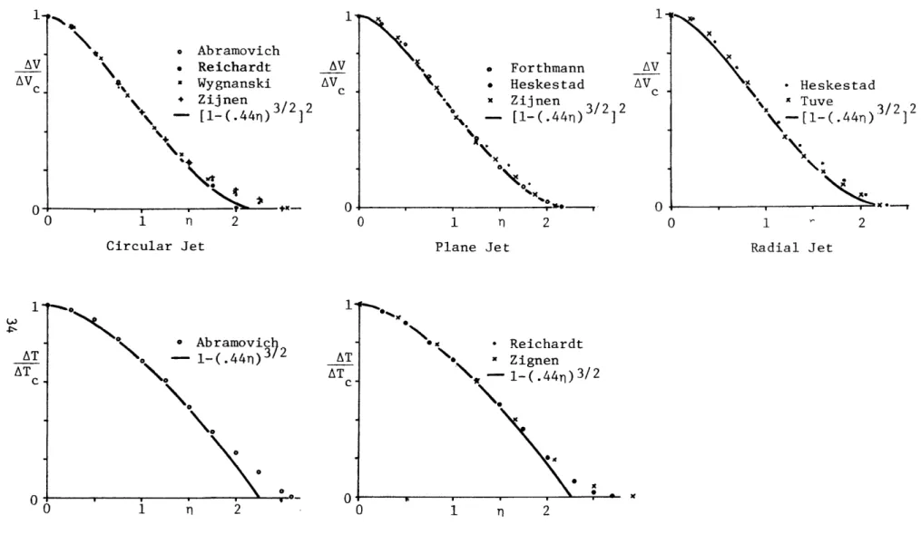
Many investigators have measured lateral velocity profiles for each of the jet discharge geometries. An important result is that the velocity profile shape (f(n)) is reasonably independent of the jet geometry considered (see Figure 2-5). The temperature profile shape (g(T)) appears narrower in the circular jet than in the plane jet, though there

is some discrepancy among researchers. Radial jet temperature profiles have apparently not been studied.

The profiles appear in integral jet equations as integral shape constants (Equations 2.4-2.6). The necessary constants for each geometry are defined in Table 2-2.

AVV AV c I-0₀ o Abramovich * Reichardt . Wygnanski + Zijnen _{3/2 2} -- [1-(.44) ] AV AV N 0-n 2 Circular Jet 0x _{* Forthmann} * Heskestad x 7 n - LJ..L 0[ - [-NX qn_

(

\o0

o

\.

Figure 2-5 Non-Buoyant Jet Mean Profile Data Compared to Polynomial Profiles 4-. AT AT C 0* 1 n 2 0,

-Radial or Plane Jet I =o f(n)dnr 12 = fo f (n) 2 d n 2 f 0 n)"d Jl = f g ()dn J2 o g(n) dn K₁ = fo g(n)f(n)dn 0 o Circular Jet Ii* = ₀ nff(n)dn 12" - fo nf(n)2dn Jl * = fo ng(n)dn J2*= fo ng(n) 2dn K * =

f

Table 2-2 Integral Shape Constants

Table 2-3 lists constant values determined experimentally and by using

two assumed profile forms:

Polynomial Profiles AT = f() = [1 - (.441In )3 / 2 c = 0 AT 3/ AT= g(n) = 1 - (.4411ni) /2 c =0 for - 2.27 < n < 2.27 for Inj > 2.27 for - 2.27 < n < 2.27 for In! > 2.27 Exponential Profiles AV = exp (- .693 n 2 ) AV c AT 2 /y2) AT= exp (- .693

n

where y is the ratio of the width bT (where temperature difference reaches half of its centerline value) to b .

(2.10)

2.4.1.3 Closure Relation Data

For the plane and circular jet geometries, the choice between a spreading or an entrainment closure equation is immaterial. A constant spreading rate, ENB,necessitates a constant entrainment coefficient, a. With spreading, flow, and conservation of momentum equations, Jirka

et al. (1975) derive

dbdb₁ 2a

dx NB plane jets (2.14)

E circular jets (2.15)

NB I1*

For the radial jet discharge geometry, a constant spreading rate and a constant entrainment coefficient give different results. The

expression analogous to Eq. 2.14 or 2.15 is

2a b

e _NB 2 _I - b _r (2.16)

A constant ENB implies b2 is proportional to x (or r-ro). Thus b /r, and consequently a must change along the jet path (Figure 2-6).

Experimental studies have determined the spreading rate eNB by measuring lateral velocity profiles. eNB is found to have a nearly constant value along the jet path for each of the three geometries1 Considering the scatter of experimental values in Table 2-3, ENB is

also essentially constant among the three geometries. Temperature profile spreading and jet boundary spreading (b T and b) are also noted in Table 2-3.

iHeskestad (1965) indicates a 10% increase in the value of ENB for a plane AV

jet for c

< .43. V_o

b₂ P b E X b ENB x = ENB(r-ro) Figure 2-6 Source (r +x')/D _o 0 0 x Heskestad w Witze 46. 33. 44. 87. 92. f" 210.

Radial Jet Spreading

NB=

.105-..

Figure 2-7 Radial Jet Spreading Data and Closure Assumptions

15-10. D o 0 0

______rmllYLI__II_(I _~---iT-i --i~W1I1-i~i~_-(l~ l-L1-

--_ 1

db b 'NB dx b, biT I1 T 1 ₂ K₁ Witze (1976) .106 _ Heskestad (1966) .110 1.10 0.78 Radial Tuve (1953) _ 1.81a 1.06 0.77

Jet Polynomial Profiles 1.43 1.02 0.72 1.36 1.02 0.84

Exponential Profiles 1.06 0.75

Kotsovinos (1975) .108 1.40 ₁.₀₆b ₀.₇₅b ₁._{4 9}b ₁.₀₅b ₀._{8 8}b

Heskestad (1965) .110 1.77 1.07 0.76

Plane v.d. Hegge Zijnen (1957) .098 1.45 1.05 0.76 1.44 1.06 0.87

Jet Reichardt (1951) 1.45 1.40 1.03 0.84c Forthmann (1934) .099 1.05 0.76 Polynomial Profiles 1.43 1.02 0.72 1.36 1.02 0.84 _ _ Exponential Profiles 1.06 0.75 ₁.5 4d 1, 08d 0.8 7d I 1 2 1 2 1 Wygnanski (1969) .088 1.85 0.75 0.37 Abramovich (1 96 3)e .097 1.43 0.68 0.36 1.24 0.71 0.47 Reichardt (1951) 0.73 0.35 Circular Albertson (1950) .097 Jet Hinze (1948) .094 1.17 0.77 0.37 ₀.8 4b 0.4 9b 0.4 2b Corrsin (1946) .084 1.20 Polynomial Profiles 1.43 0.66 0.34 1.10 0.66 0.46 Exponential Profiles 0.72 0.36 0.85f 0.50 0.42 Notes:

a. Actually db/dx was measured, values reflect Heskestad's value for db/ dx

b. Uses author's fitted exponential profiles

c. Reichardt temperature data with polynomial velocity profile d. Uses mean experimental value of b,/lb.

e. Based on review of many Russian aiad Grman studies

f. Uses value of b l/b! = 1.18

Table 2-3 Experimental Data for Unconfined, Nonbuoyant Jets

Geometry Sources

o

2.4.1.4 Radial Jet Behavior

Radial jet data from Witze (1976), Heskestad (1966), and Tuve (1953) strongly support a closure assumption of a constant spreading rate, inde-pendent of A (Figure 2-7). _{The measured spreading rate is also essentially} equal to the plane jet value. A constant entrainment coefficient

would be inconsistent with observed non-buoyant radial jet behavior.

Because experimental values for plane and radial jets are indis-tinguishable in Table 2-3, plane jet data will be used to supplement radial jet data. This practice will be even more imperative in succeeding

sections.

Heskestad (1965) suggests the existence of two slightly different AV

plant jet spreading rates, with a transition at V- Z .43. Forthmann (1934)

0

and v.d. Hegge Zijnen (1957) measured jet properties in the region where AV

c > .43. Heskestad (1965) and Kotsovinos (1975) primarily measured Vo

AV c

spreading at greater distances for which c < .43. A spreading relation exhibiting this transition is:

AV

NB = .105 + .005 tanh[(.43 - c) / . 0 2 8 ] (2.17)

2.4.2 Zone of Flow Establishment

An unsheared core of fluid distinguishes spreading in this zone from fully developed jet spreading (Figure 2-2). Lateral velocity and temperature profiles and a closure relation are still required for an integral jet model. An appropriate closure relation is the decay of the unsheared half-width, dD/dx.

Albertson et al. (1950) is one of the few studies with detailed 39

^~~I~-measurements in this relatively short zone. However experimental work on turbulent shear layers (Figure 2-8) can be applied. Jet establishment

or shear layer experimental results can be used until the core disappears (D=O) and before switching to the fully developed jet relations of

Section 2.4.1. However some transition must occur between the two regions and their different spreading rates.

2.4.2.1 Paramerization

This region is governed by the same non-buoyant jet parameters discussed in Section 2.4.1.1. The initial flow rate, Q , is much more important to the observed behavior in this zone than for the fully developed jet.

2.4.2.2 Profile Data

Flow establishment zones and shear layers in the radial geometry have not been studied. However there is sufficient data for the plane jet geometry. The mean velocity profiles in the sheared region have the same shape and integration constants as found for the fully developed jet (Figure 2-8 and Table 2-4). The mean velocity in the core region is simply the discharged value, V .

Sheared temperature difference profiles spread more quickly (than velocity profiles) into both the quiescent and the moving fluid. Jet centerline temperature differences are reduced to below the discharge value well before the velocity core disappears (v.d. Hegge Zignen 1957).

The turbulence measurements of Wygnanski find b/b significantly different from fully developed jet profiles.

Y

.m)

0.

Liepmann and Laufer (1947) Data

Ux

N

\

*

0 1 n 2

Liepmann & Laufer Albertson et al.

[1-(.44n) 3/21

Plane Shear Layer Mean Profile Data

AV V

o

0

2.4.2.3 Spreading Relation

Albertson et al. (1950) and Liepmann (1947) observed almost equal spreading rates (Table 2-3, Figure 2.8) with jets and shear layers respectively. If dD/dx is assumed constant, then momentum conservation (between the

discharge point and the end of the flow establishment region) may be written as

D = b1 = (D + .031 L)*I 2 (2.18)

D = .031/( - ) - .095 _(2.19)

dx I2

where L is the length of the velocity core. This is close to Albertson's published value of -. 097.

The.present study found that the following relationships are more 1

accurate as part of an overall integral jet model:

d(D+b ')

(D+ = .025 (2.20)

d= - .07

(2.21) dx

An overall integral jet model applies the fully developed jet relations as soon as the core disappears without considering any transition

between zones. The revised equations (2.20 and 2.21) enable the overall integral jet model to better model jet behavior in the transition between zones and beyond (x > L).

2.4.2.4 Radial Jet Behavior

Plane jet velocity profile coefficients from Table 2-4 are applied

1

the data of plane and radial jet data of Heskestad were primarily used for comparison.

d(D+b) _b hbT

Geometry Source dx b b 1 2 1 2 K

Plane Shear Wygnanski (1970) ._{04 8}a 1.36 Layer Albertson (1950) .032 1.03 .76 Liepmann (1947) .029 1.05 0.79 Polynomial Profiles 1.43 1.02 0.72 1.36 1.02 0.84 Exponential Profiles 1.06 0.75 1.36b 1.08b 0.84b Notes:

a. Because of experimental conditions, probably not applicable to flow establishment of jets b. Used experimental value of byT/b

Table 2-4 Experimental Data for Plane Shear Layer

to the sheared regions in the zone of flow establishment of a radial jet. These are essentially the same as those found in the fully developed radial jet. Velocity in the core is uniform at the discharged value Vo

The easiest assumption (and perhaps best because of a lack of data) about temperature profiles is that temperature differences also have a core width D. However, the core temperature difference, while uniform, is not fixed at any value. The sheared profile shapes on either side of the core must rely on fully developed plane jet data.

Unlike the profile conclusions, a plane jet spreading relation is probably not directly applicable to radial jets. The core width (D) of the radial jet would be expected to decrease with x even without turbulent shear effects (because of the increasing radial coordinate). With no radial jet data available, a plausible assumption is that the lateral area of the core region decreases at the same rate as in a plane jet. Thus d(2rD) _{- 0.07 *} 27r dr dD D d= - 0.07 -(2.22) dr r _~ I _L__^_3_~CR*nl_________^L

x

x

b

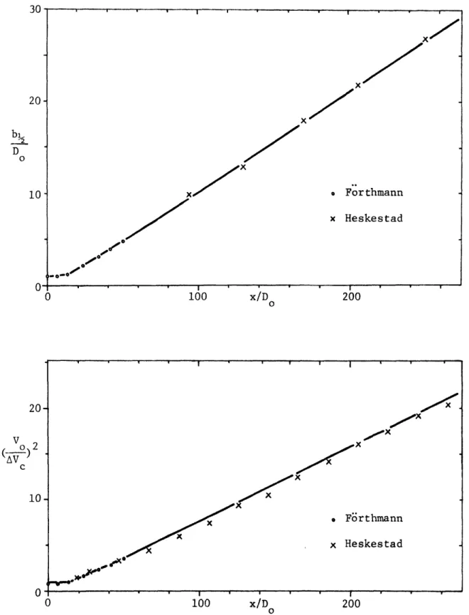
Figure 2-9 Non-Buoyant Plane Jet Integral Model Results

0 100 x/D 200 0 i I I o Frthmann x Heskestad

I

I

-I

1

I

~

-

-

--

-

_ -

_---Cc ,'OV

15 D 0 10-5 0 x/D 100

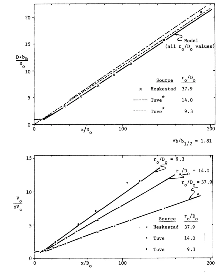
Non-Buoyant Radial Jet x/Do 15-= 1.81 104 V o AV C n r /D =9.3 0 0 r /D = 14.0 o *r /D ₌ 37.9 0 0 000.OSource 0 0 x Heskestad 37.9 x * Tuve 14.0 o Tuve 0 0 200 UY I~ 1 - -- . *b/b1/2 9.3

D and hence b no longer vary linearly.

Closure and profile assumptions have now been made for both zones of plane and radial non-buoyant jets. Therefore the integral models are complete. The integral model results are compared with experimental data of jet spreading and centerline velocity decay in Figure 2-9

(plane jets) and Figure 2-10 (radial jets).

2.4.3 Co-flowing Ambient Fluids

This section will deal with non-buoyant jets discharged into uniform co-flowing velocity streams. Since radial jets in an ambient current have not been studied, plane jet data will again be used to infer radial jet behavior.

2.4.3.1 Parameterization

In the circular and plane jet geometries there are three governing dimensional parameters: M , Qo , and U . The new parameter, U , is the uniform ambient fluid velocity relative to the jet port. (In the context of the present study U₀ is the radial inward flow caused by the plant

in-take. When U is spatially variable, Uo denotes a reference value.) One dimensionless parameter governs behavior.

IV = M o /Qo*U _o (2.23)

0

2.4.3.2 Profile Data

The profile shape of excess velocity (velocity above ambient velocity) is identical to the velocity profile of Section 2.4.1. Data from Weinstein (1957) are presented in Figure 2-11. Temperature difference profiles also have shapes similar to jets in nonflowing ambient fluids. This makes all the profile integrals of Table 2-5 the same as well.

*Weinstein -_-[l-(.4 4n)

I

S

Figure 2-11 Co-flowing Jet Mean Profile Data

.12 .11 Data o x S Nh %. % t% 0 % x Abramovich Forthmann

+ Bradbury & Riley Abramovich Relations:

K = .4560

+

I

" 1

.4 Uo/V _{0 c} .6 1.0

Spreading Rate with Ambient Velocities 1 AV AVc 0 .1 .10, .09 .08 .07 *\ 0 db dx .05 .04 -. 2

~YI1---.-.

.LII-^---~

U_~IIIIIII~

-

----• •

1

1

1

Notes:

a. Actually profile data of CO2 concentration of a CO2 jet into air b. Used polynomial velocity profile

c. Used experimental value of b /b

Table 2-5 Experimental Data for Plane Co-flowing Jets

2.4.3.3 Spreading Relation

Rajaratnam (1976) includes a whole chapter on plane jets in co-flowing streams. His similarity analysis shows that jet spreading is proportional to x for 7 >> 1 (termed strong jets) and proportional to

2x for I << 1 (termed weak jets). Any discharged "strong" jet goes through a transition between these proportionalities as it becomes a weak jet. Many studies with experimental data and empirical formulas

(for spreading and centerline velocity decay) are cited by Rajaratnam. Abramovich (1963) makes a jet spreading assumption much simpler than many mentioned by Rajaratnam. This assumption fits data well -expecially for "stronger" jets. It is also extendable to counter-flowing ambient fluids (section 2.4.4) which are considerably more important

in this radial jet study.

Abramovich's argument (simply stated) is that the jet boundary moves laterally at a speed proportional to the centerline excess velocity, AV _c. At the same time, jet fluid moves ahead at an average velocity of

= [2b

+

AVdy]/2b*

48

dbb _"I

Geometry Source dx I i 2 1 '1,

Plane Bradbury (1967) f(-U-) 1.01 0.73

Co-Flowing c

Jets Abramovich (19 63)a ' 1.46 1.39 1.03 0.8 5b

Weinstein (1957) " 1.02 0.76

Polynomial Profiles 1.02 0.72 1.36 1.02 0.84 Exponential Profiles 1.06 0.75 1.55c 1.10c 0.8 8c

Ilb

= U + AVIb (2.24)

b

where b is the jet half-width over which the velocity is averaged. Jet spreading, according to Abramovich, is simply a ratio of these velocities

b AV Cc =NB (I1 *A b b U + AV I1 _b* = K (2.25) =NB x Uo/AV + K c

where sNB is the nonbuoyant jet spreading rate in a stagnant ambient and K = Ilb /b . The value of b (hence K) is a fitting coefficient. However it should be closer to b (a measure of the turbulent zone width) than b; in value.

Experimental spreading rates are plotted (Figure 2-12) with c for two values of b*

b = 2.2 b = 1.22 b (K1 = .45)

b = 1.7 b1 = 0.94 b (K2 = .60) (2.26) A2

The first value, bl, is suggested by Abramovich and it fits the data he cites (Figure 2-12, open symbols) well. The second value, b2, is a better

fit to the mean curve drawn through results of Bradbury and Riley (1967). Figure 2-13 shows the spread of co-flowing jets of various V values, The use of b2 in the spreading relation allows an integral jet model to fit

Integral Model: V -K. .45 6 --- K =.60 4

=3.12

2.4.3.4 Radial Jet Behavior

The original profile constants of section 2.4,1 appear applicable in co-flowing stream situations as well.

Radial jet spreading was found to be constant and equal to plane jet spreading in stagnant ambients. Therefore the plane jet spreading relation just derived will be applied directly to radial jets. The choice of fitting constant, K, will be determined in the next section where the same relation is applied to counter-flowing ambients.

2.4.4 Counter-Flowing Ambient Fluids

A non-buoyant jet discharging into an unbounded uniform counterflow must eventually be "blown" back upon itself. For this reason jet

boundaries and other behavior are not easily discerned (Figure 2-14). The relatively scarce data for this situationare for the circular jet geometry only.

2.4.4.1 Parameterization

The parameters and dimensionless number are exactly the same as for the co-flowing case. Only the sign of U0 has changed.

2.4.4.2 Profile Data

Both Rajaratnam (1976) and Abramovich (1963) refer to circular jet studies. Only Abramovich displays excess velocity (above ambient velocity) profile data from the work of Vulis (1955). The unconfined, non-buoyant jet profile shape is again apparent in Figure 2-14.

2.4.4.3 Spreading Relation

The main concern in the experiments cited was for the jet

Xp Velocity Field 1 -AV AV c o0 So Abramovich - (1(.44n)3/2) 2 . 0 0 0 I * I 0 1 2

Excess Velocity Profile

tion distance, X p. Spreading measurements were not made or were not

reported completely.

A circular, ducted jet study by Becker, Hottel, and Williams (1962)

provides the best data for jet spreading in counter-flowing ambient fluids. Because this is a confined jet situation, the ambient velocity is decreasing or becoming more negative as the jet moves away from its discharge point (Figure 1-3). The governing parameters now include Hi, the radius of the duct wall. This means a second dimensionless governing parameter is needed:

I M / 2U 2 (2.27)

However Becker et al. measured the centerline velocity, AVc, the ambient velocity, U, and the jet width b; at various sections. Therefore

equation 2.25 can be applied for average values of AVc and U between sections to predict the increase in b. In this way the more

complicated experiment is analyzed as a series of uniform counter-flowing ambient fluid situations.

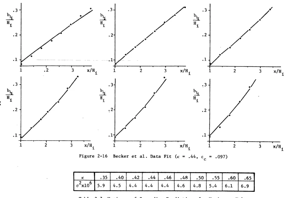
The spreading results of six experiments by Becker et al. (1962) appear in Figure 2-15. Velocity and jet width data appear in the

accompanying Table 2-6. It is apparent that spreading is greatest for the highest values of 1 - those experiments in which ambient counter velocities occur earliest and with the largest magnitudes. Various values of K were tried in Eq. 2.25 (with cNB = .097) to fit the data.

The best fit was for K = .44 which is almost equal to the Abramovich suggestion of .45 (Figure 2-16). Table 2-7 lists the variance of jet

I I I I .3 0 7 1/I .2 .1 I 1 I 4 0 1 2 x/Hi 3 4

Figure 2-15 Circular Ducted Jet Spreading Hi * I - 1300. * =I 560. x

IM -

130.

A I4

=

31.

Exp. No. x/Hi 1.01 1.42 1.79 2.19 2.57 2.96 3.36 3.76

#1 U b /Hi .081 .114 .146 .174 .206 .241 .276 .305 IM= 9.3 U +1.13 +1.09 +1.07 +0.q3 +0.86 +0.79 +0.79 +0.71 AV 13.62 9.54 7.34 6.06 5.24 4.46 4.03 3.60 #2 4a b1/Hi .083 .120 .150 .182 .213 .250 .278 .310 1M= 31. U +0.64 +0.55 +0.52 +0.49 +0.46 +0.43 +0.37 +0.16 AV 13.62 9.54 7.34 6.06 5.24 4.46 3.94 3.56 43 k b1/Hi .086 .122 .151 .188 .223 .263 .305 .349 11= 130. U +0.29 +0.28 +0.26 +0.21 +0.11 -0.18 -0.31 AV 13.62 9.54 7.34 6.06 5.24 4.72 4.26 3.98 #4 + b /Hi .088 .124 .159 .188 .229 .284 .331 14= 560. U +0.02 -0.01 -0.15 -0.20 -0.31 -0.47 -0.52 AV 13.1 9.1 7.11 6.52 5.42 4.74 4.16 #5 .o" b /Hi _,I .089 .127 .167 .211 .267 .330 14= 1300. U -0.04 -0.13 -0.22 -0.32 -0.45 -0.55 AV 13.0 9.0 7.11 5.74 4.76 4.14 16 "" bi/Hi .094 .132 .180 .236 .294 .353 N= 00 U -0.26 -0.35 -0.43 -0.52 -0.61 -0.70 -0.82 AV 12.67 8.93 6.79 5.29 4.50 3.82 3.33 Table 2-6 Circular Ducted Jet Data (Becker et al., 1962)

, v .3-Hi .2-.1 -.3 H_i b2 H.1

.3-o//

2/x

o.7-.7

/

0"

0

0//

Figure 2-16 Becker et al. Data Fit (K = .44, c = _.097)

< ,35 .40 .42 .44 .46 .48 .50 .55 .60 .65

C2x106 5.9 4.5 4.4 4.4 4.4 4.6 4.8 5.4 6.1 6.9

Table 2-7 Variance of Spreading Predictions for Various K Values

Hi 1 .2 3 x/H

/

.1-2.4.4.4 Radial Jet Behavior

As in the previous section, jet profile results in Section 2.4.1 are applicable. The appropriate spreading relation appears to be equation 2.25 with K = 0.44. The non-buoyant spreading rate, ENB' should be the relation found applicable to plane and radial jets in Section 2.4.1.

AV .44

Ec = {.105 + .005 tanh[(.43 -- c V c)/.028]} . U/AV + .44 (2.28)

It should be remembered that the experiments by Becker et al. (1962) had turbulent counterflowing ambient fluid. This may cause spreading somewhat different from that observed in the detached jet of this study (where the ambient flow is irrotational).

2.4.5 Buoyant Unconfined Jets

As in other sections, the radial geometry for this situation has apparently not been studied. Geometrical similarities and the equivalence of spreading rates for plane and radial jets was noted in Section 2.4.1. Therefore buoyant plane jet data will be emphasized and then assumed to apply to the radial case.

An important property of these jets is that (in an unstratified ambient fluid) their behavior eventually becomes that of a pure plume as buoyancy overcomes initial momentum effects,

2.4.5.1 Parameterization

Buoyancy adds a new governing parameter, Bo, to those of the unconfined non-buoyant jet. Also the directional nature of the buoyancy

force makes 0 or the jet discharge angle important (horizontal discharge:

o = 0_{*; vertical discharge:}

o = 900). Thus the following dimensionless

numbers result:

1. o initial jet angle to the horizontal (2.29)

2. F ' = [M 3/B

oQ

or

F = [Mo 5/2/B o]/2 radial or circular jet densimetric

Froude number (2.30)

3. A= ro

M/Q

Pure plume spreading (Mo = 0 and o = 90°) has two governing

parameters (Bo and Qo) and no dimensionless numbers. Therefore the

property of jet spreading (or the entrainment coefficient) should be the same for all plumes (just as is the case for a non-buoyant jet with governing parameters of Mo and Qo ).

Only three major studies were found of a plane plume. Rouse et al. (1952) studied the pure plane "plume" (M_° = 0) created from a

heat source. The jets of Kotsovinos (1975) had initial momentum but were all discharged vertically (4o = 90*) and did not bend. Cederwall

(1971) considered a horizontal discharge. However experimental boundaries made his jets somewhat confined. Cederwall's results will be discussed