Instantaneous frequencies of a chaotic system
10
0
0
Texte intégral
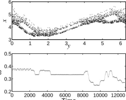
Figure

Documents relatifs