Inter-subject pattern analysis A straightforward and powerful scheme for group-level MVPA

(1)

HAL Id: hal-02313840

https://hal.archives-ouvertes.fr/hal-02313840

Submitted on 11 Oct 2019

HAL is a multi-disciplinary open access

archive for the deposit and dissemination of

sci-entific research documents, whether they are

pub-lished or not. The documents may come from

teaching and research institutions in France or

abroad, or from public or private research centers.

L’archive ouverte pluridisciplinaire HAL, est

destinée au dépôt et à la diffusion de documents

scientifiques de niveau recherche, publiés ou non,

émanant des établissements d’enseignement et de

recherche français ou étrangers, des laboratoires

publics ou privés.

Inter-subject pattern analysis A straightforward and

powerful scheme for group-level MVPA

Qi Wang, Bastien Cagna, Thierry Chaminade, Sylvain Takerkart

To cite this version:

Qi Wang, Bastien Cagna, Thierry Chaminade, Sylvain Takerkart. Inter-subject pattern analysis A

straightforward and powerful scheme for group-level MVPA. NeuroImage, Elsevier, 2019, pp.116205.

�10.1016/j.neuroimage.2019.116205�. �hal-02313840�

(2)

Inter-subject pattern analysis

A straightforward and powerful scheme for group-level MVPA

Qi Wanga,b_{, Bastien Cagna}a_{, Thierry Chaminade}a_{, Sylvain Takerkart}?a

?_{Corresponding author: Sylvain.Takerkart@univ-amu.fr}

https: // doi. org/ 10. 1016/ j. neuroimage. 2019. 116205

a_{Institut de Neurosciences de la Timone UMR 7289, Aix-Marseille Université, CNRS} Faculté de Médecine, 27 boulevard Jean Moulin, 13005 Marseille, France

b_{Laboratoire d’Informatique et Syst`emes UMR 7020, Aix-Marseille Universit´e, CNRS, Ecole Centrale de Marseille}

Facult´e des Sciences, 163 avenue de Luminy, Case 901, 13009 Marseille, France

Abstract

Multivariate pattern analysis (MVPA) has become vastly popular for analyzing functional neuroimaging data. At the group level, two main strategies are used in the literature. The standard one is hierarchical, combining the outcomes of within-subject decoding results in a second-level analysis. The alternative one, inter-subject pattern analysis, directly works at the group-level by using, e.g. a leave-one-subject-out cross-validation. This study provides a thorough comparison of these two group-level decoding schemes, using both a large number of artificial datasets where the size of the multivariate effect and the amount of inter-individual variability are parametrically controlled, as well as two real fMRI datasets comprising 15 and 39 subjects, respectively. We show that these two strategies uncover distinct significant regions with partial overlap, and that inter-subject pattern analysis is able to detect smaller effects and to facilitate the interpretation. The core source code and data are openly available, allowing to fully reproduce most of these results.

Keywords: fMRI, MVPA, group analysis

1. Introduction

Over the past decade, multi-voxel pattern analysis (MVPA, [15]) has become a very popular tool to extract knowledge from functional neuroimaging data. The advent of MVPA has offered new opportunities to examine neural coding at the macroscopic level, by making explicitly usable the information that lies in the differential modulations of brain activation across multiple locations – i.e. multiple sensors for EEG and MEG, or multiple voxels for functional MRI (fMRI). Multivariate pattern analy-sis commonly conanaly-sists in decoding the multivariate information contained in functional patterns using a classifier that aims to guess the nature of the cognitive task performed by the partici-pant when a given functional pattern was recorded. The decod-ing performance is consequently used to measure the ability of the classifier to distinguish patterns associated with the different tasks included in the paradigm. It provides an estimate of the quantity of information encoded in these patterns, which can then be exploited to localize such informative patterns and/or to gain insights on the underlying cognitive processes involved in these tasks.

This decoding performance is classically estimated sepa-rately in each of the participants. At the group level, these within-subject measurements are then combined – often using a t-test – to provide population-based inference, similarly to what is done in the standard hierarchical approach used in activation studies. Despite several criticisms of this group-level strategy that have been raised in the literature (see herafter for details),

this hierarchical strategy remains widely used.

An alternative strategy directly works at the group-level by exploiting data from all available individuals in a single analy-sis. In this case, the decoding performance is assessed on data from new participants, i.e. participants who did not provide data for the training of the classifier (see e.g. [32, 17, 19, 20, 18, 10]), ensuring that the nature of the information is consis-tent across all individuals of the population that was sampled for the experiment. This strategy takes several denominations in the literature such as across-, between- or inter-subject clas-sification or subject-transfer decoding. We hereafter retain the name inter-subject pattern analysis (ISPA).

In this paper, we describe a comparison of the results pro-vided by these two classifier-based group-level decoding strate-gies with both artificial and real fMRI datasets, which, to the best of our knowledge, is the first of its kind. This experimental study was carefully designed to exclusively focus on the di ffer-ences induced by the within- vs. inter-subject nature of the de-coding, i.e. by making all other steps of the analysis workflow strictly identical. We provide results for both two real fMRI datasets and a large number of artificial datasets where the char-acteristics of the data are parametrically controlled. This allows us to demonstrate that these strategies offer different detection power, with a clear advantage for the inter-subject scheme, but furthermore that they can provide results of different nature, for which we put forward a potential explanation supported by the results of our simulations on artificial data. The paper is

(3)

orga-nized as follows. Section 2 describes our methodology, includ-ing our multivariate analysis pipeline for the two group-level strategies, as well as a description of the real datasets and the generative model of the artificial datasets. Section 3 includes the comparison of the results obtained with both strategies on these data, both in a qualitative and quantitative way. Finally, in Section 4, we discuss the practical consequences of our results and formulate recommendations for group-level MVPA.

2. Methods

2.1. Group-MVPA (G-MVPA)

Since the seminal work of [16] that marked the advent of multivariate pattern analysis, most MVPA studies have relied on a within-subject decoding paradigm. For a given subject, the data is split between a training and a test set, a classifier is learnt on the training set and its generalization performance – usually measured as the classification accuracy – is assessed on the test set. If this accuracy turns out to be above chance level, it means that the algorithm has identified a combination of fea-tures in the data that distinguishes the functional patterns asso-ciated with the different experimental conditions. Said other-wise, this demonstrates that the input patterns contain informa-tion about the cognitive processes recruited when this subject performs the different tasks that have been decoded. The de-coding accuracy can then be used as an estimate of the amount of available information – the higher accuracy, the more distin-guishable the patterns, the larger the amount of information.

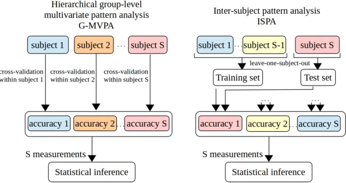
The group-level extension of this procedure consists in eval-uating whether such information is present throughout the pop-ulation being studied. For this, a second level statistical analysis is conducted, for instance to test whether the average classifica-tion accuracy (or any other relevant summary statistic measured at the single-subject level), computed over the group of partic-ipants, is significantly above chance level. This can be done using a variety of approaches (see 2.6 for references). This hi-erarchical scheme is the one that is most commonly used in the literature. We denote it as Group-MVPA (G-MVPA) in the rest of the present paper and illustrate it on Figure 1.

2.2. Inter-Subject Pattern Analysis (ISPA)

Besides the hierarchical G-MVPA solution, another classifier-based framework exists to evaluate multivariate effects at the group level. Considering the data from all available individu-als, one can train a classifier on data from a set of subjects – the training subjects – and evaluate its generalization capability on data from the others – the test subjects. One can then use a cross-validation scheme that shuffles the subjects between the training and test sets, such as leave-one-subject-out or leave-n-subjects-out. In this setting, obtaining an average classification accuracy – this time across folds of the cross-validation – signif-icantly above chance level means that a multivariate effect has been identified and that it is consistent across individuals. We denote this strategy as Inter-Subject Pattern Analysis (ISPA).

In this study, we use a leave-one-subject-out cross-validation in which the model accuracy is repeatedly computed on the

data from the left-out subject. Even if other schemes might be preferable to multiply the number of measurements [34], this choice was made to facilitate the comparison of the results ob-tained with ISPA and G-MVPA, as illustrated on Figure 1.

2.3. Artificial data

The first type of data we use to compare G-MVPA and ISPA is created artificially. We generate a large number of datasets in order to conduct numerous experiments and obtain robust re-sults. Each dataset is composed of 21 subjects (for ISPA: 20 for training, 1 for testing), with data points in two classes labeled as Y = {+1, −1}, simulating a paradigm with two experimen-tal conditions. For a given dataset, each subject s ∈ {1, 2, ..., 21} provides 200 labeled observations, 100 per class. We denote the i-th observation and corresponding class label (xs

i, y s i), where xs i ∈ R 2_{and y}s i ∈ Y. The pattern x s i is created as x_is= cos θ s _{− sin θ}s sin θs _{cos θ}s ! ˜x_is, where • ˜xs

i is randomly drawn from a 2D Gaussian distribution,

N (C+, Σ) and N(C−_{, Σ) if y}s

i = +1 or y s

i = −1,

respec-tively, which are defined by their centers C+ = (+d₂, 0) and C− _{= (−}d

2, 0), where d ∈ R+ and their covariance

matrixΣ, here fixed to 1 0 0 5 !

(see Supplementary Mate-rials for results with other values ofΣ);

• θs_{defines a rotation around the origin that is applied to all}

patterns of subject s; the value of θs is randomly drawn from the Gaussian distribution N(0,Θ), where Θ defines the within-population variance.

Let Xs _{= (x}s i) 200 i=1 and Y s_{= (y}s i) 200

i=1 be the set of patterns and

labels for subject s. A full dataset D is defined by

D=

s=21

[

s=1

{Xs, Ys}.

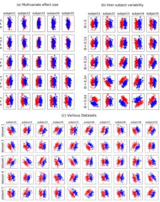
The characteristics of such a dataset are in fact governed by two parameters:

• d, which defines the distance between the point clouds of each of the two classes, i.e. the multivariate effect size; • Θ, which controls the amplitude of the rotation that can

be applied to the data, separately for each subject: when Θ is small, all the θs_{angles remain small, which means}

that the data of all subjects are similar; whenΘ increases, the differences between subjects become larger; there-fore,Θ quantifies the amount of inter-individual variabil-ity that exists within the group of 21 subjects for a given dataset.

Figures 2a and 2b illustrate the influence of each of these two parameters. Figure 2c shows different datasets generated with the same values of d andΘ.

(4)

Figure 1: Illustration of the two approaches available to perform classifier-based group-level multivariate analysis. Left: hierarchical group-MVPA (G-MVPA). Right: inter-subject pattern analysis (ISPA). Note that if a leave-one-subject-out cross validation is used for ISPA (as illustrated), the two approaches yield the same number of measurements (equal to the number of subjects S ), which allows for an unbiased comparison using the same statistical inference method.

In our experiments we used 13 values for d and 11 values for Θ, d ∈ {0.1, 0.12, 0.14, 0.16, 0.18, 0.2, 0.22, 0.24, 0.26, 0.28, 0.3, 0.4, 0.6},Θ ∈ {0.2π, 0.25π, 0.3π, 0.35π, 0.4π, 0.45π, 0.5π, 0.55π, 0.6π, 0.65π, 0.7π}, which gives 143 points in the two dimen-sional parameter space spanned by d andΘ. Note that by chang-ing the value ofΘ while keeping Σ constant, we control the rel-ative amounts of within- and between-subject variance, which have been shown to be critical in group-level decoding situa-tions [24]. For each pair (d,Θ), we generated 100 datasets. This yields 14300 datasets, each comprising 21 subjects and a total of 4200 data points. The code for generating these datasets (as well as performing the experiments detailed hereafter) is avail-able online at the following URL: http://www.github.com/ SylvainTakerkart/inter_subject_pattern_analysis.

2.4. fMRI data

We also used two real fMRI datasets that were acquired at the Centre IRM-INT in Marseille, France. For both experi-ments, participants provided written informed consent in agree-ment with the local guidelines of the South Mediterranean ethics committee.

In the first experiment (hereafter Dataset1), fifteen subjects participated in an investigation of the neural basis of cognitive control in the frontal lobe, largely reproducing the experimen-tal procedure described in [21]. Participants lying supine in the MRI scanner were presented with audiovisual stimuli that required a button response, with the right or left thumb. Four inter-stimulus intervals were used equally in a fully randomized

order (1.8, 3.5, 5.5, 7.1 seconds), with an average of 4.5 sec-onds over a session. Data was collected with a 3T Bruker Med-spec 30/80 Avance scanner running ParaVision 3.0.2. Eight MRI acquisitions were performed. First, a field map using a double echo Flash sequence recorded distortions in the mag-netic field. Six sessions with 60 trials each were recorded, each comprising 133 volumes (EPI sequence, isotropic resolution of 3 × 3 × 3 mm, TE of 30 ms, flip angle of 81.6◦, field of view of 192 × 192 mm, 36 interleaved ascending axial slices acquired within the TR of 2400 ms) encompassing the whole brain paral-lel to the AC-PC plane. Finally, we acquired a high-resolution T1-weighted anatomical image of each participant (MPRAGE sequence, isotropic voxels of 1 × 1 × 1 mm, field of view of 256 × 256 × 180 mm, T R= 9.4 ms, T E = 4.424 ms).

In the second experiment (Dataset2), thirty-nine subjects were scanned using a voice localizer paradigm, adapted from the one analyzed in [29]. While in the scanner, the participants were asked to close their eyes while passively listening to a set of 144 audio stimuli, half of them being voice sounds, the other half being non-vocal. Most of the stimuli were taken from a database created for a previous study [6], while the others were extracted from copyright-free online databases. The paradigm was event-related, with inter-stimulus intervals randomly cho-sen between 4 and 5 seconds. The images were acquired on a 3T Prisma MRI scanner (Siemens, Eerlangen, Germany) with a 64-channels head coil. A pair of phase-reversed spin echo images was first acquired to estimate a map of the magnetic field. Then, a multi-band gradient echo-planar imaging (EPI)

(5)

Figure 2: Illustration of the artificial datasets generated with the model described in 2.3. Each line is a subpart of a single dataset (5 subjects shown amongst 21 in (a) and (b), 10 subjects shown in (c)). The data points belonging to the class y = +1 and y = −1 are shown in blue and red, respectively. (a): influence of the d parameter (increasing effect size from top to bottom). (b): influence of the Θ parameter (increasing inter-individual variability from top to bottom). (c) five datasets obtained with the same values of the two parameters (d= 2 and Θ = 0.2π).

sequence with a factor of 5 was used to cover the whole brain and cerebellum with 60 slices during the TR of 955 ms, with an isotropic resolution of 2 × 2 × 2 mm, a TE of 35.2 ms, a flip angle of 56 degrees and a field of view of 200 × 200 mm for each slice. A total of 792 volumes were acquired in a single run of 12 minutes and 36 seconds. Then, a high resolution 3D T1 image was acquired for each subject (isotropic voxel size 0.8 mm3, T R = 2400 ms, T E = 2.28 ms, field of view of 256 × 256 × 204.8 mm). Dataset2 is part of the InterTVA data set [1], which is fully available online1.

2.5. fMRI data analysis

The two datasets were processed using the same sets of op-erations. The pre-processing steps were performed in SPM122. They included co-registration of the EPIs with the T1 anatom-ical image, correction of the image distortions using the field

1_{https://openneuro.org/datasets/ds001771} 2

https://www.fil.ion.ucl.ac.uk/spm/

maps, motion correction of the EPIs, construction of a population-specific anatomical template using the DARTEL method, trans-formation of the DARTEL template into MNI space and warp-ing of the EPIs into this template space. Then, a general linear model was set up with one regressor per trial, as well as other regressors of non interest such as motion parameters, following the least-squares-all approach described in [26]. The estimation of the parameters of this model yielded a set of beta maps that was each associated with a given experimental trial. The beta values contained in these maps allowed constructing the vec-tors that serve as inputs to the decoding algorithms, that there-fore operate on single trials. We obtained 360 and 144 beta maps per subject for Dataset1 and Dataset2 respectively. No spatial smoothing was applied on these data for the results pre-sented below (the results obtained with smoothing are provided as Supplementary Materials).

For these real fMRI datasets, we performed a searchlight decoding analysis [23], which allows to map local multivari-ate effects by sliding a spherical window throughout the whole brain and performing independent decoding analyses within each sphere. For our experiments, we exploited the searchlight im-plementation available in nilearn3_{to allow obtaining the}

single-fold accuracy maps necessary to perform inference. For Dataset1, the decoding task was to guess whether the participant had used his left vs. right thumb to answer during the trial corresponding to the activation pattern provided to classifier. For G-MVPA, the within-subject cross-validation followed a leave-two-sessions-out scheme. For Dataset2, the binary classification task con-sisted in deciphering whether the sound presented to the partic-ipant was vocal or non-vocal. For G-MVPA, because a single session was available, we used an 8-fold cross-validation. Fi-nally, all experiments were repeated with five different values of the searchlight radius (r ∈ {4 mm, 6 mm, 8 mm, 10 mm, 12 mm}).

2.6. Classifiers, Statistical inference and performance evalua-tion

In practice, we employed the logistic regression classifica-tion algorithm (with l2regularization and a regularization weight

of C = 0.1), as available in the scikit-learn4 python module, for both artificial and real fMRI data. The logistic regression has been widely used in neuroimaging because it is a linear model that enables neuroscientific interpretation by examining the weights of the model, and because it provides results on par with state of the art methods while offering an appealing com-putational efficiency [30].

In order to perform statistical inference at the group level, the common practice is to use a t-test on the decoding accu-racies. Such a test assesses whether the null hypothesis of a chance-level average accuracy can be rejected, which would re-veal the existence of a multivariate difference between condi-tions at the group level (note that, as detailed in 2.1 and 2.2, the rejection of this null hypothesis provides different insights on

3_{http://nilearn.github.io/} 4

(6)

the group-level effect depending on whether G-MVPA or ISPA is used).

However, several criticisms have been raised in the liter-ature against this approach, namely on the nliter-ature of the sta-tistical distribution of classification accuracies [28, 2], on the non-directional nature of the identified group-information [13] or on the fact that the results can be biased by confounds [33]. This has led to the development of alternative methods (see e.g. [28, 5, 31, 9, 2]), all dedicated to G-MVPA.

Because our objective is to compare the results given by G-MVPA and ISPA in a fair manner, i.e using the same statistical test, we used a permutation test [27] which allows overcom-ing some of the aforementioned limitations. This test assesses the significance of the average accuracy at the group-level in a non-parametric manner for all the experiments conducted in the present study, whether conducted with G-MVPA or ISPA. Fur-thermore, this choice allowed maintaining the computational cost at a reasonable level, a condition that other alternatives, e.g inspired by [31], would not have met (see the Supplementary Materials for a longer discussion on this matter). In practice, for the real fMRI experiments, we used the implementation of-fered in the SnPM toolbox5_{to analyse the within-subject (for}

G-MVPA) or the single-fold (for the inter-subject cross-validation of ISPA) accuracy maps, with 1000 permutations and a signif-icance threshold (p < 0.05, FWE corrected). For the simula-tions that used the artificial datasets, we used an in-house im-plementation of the equivalent permutation test (also available in our open source code; see 2.3), with 1000 permutations and a threshold at p < 0.05. Critically, it should be noted that the same number of samples were available for this statistical pro-cedure when using G-MVPA or ISPA, as shown on Figure 1.

In order to compare the group-level decoding results pro-vided by G-MVPA and ISPA, we use the following set of met-rics. For the artificial data, we generated 100 datasets at each of the 143 points of the two dimensional parameter space spanned by the two parameters d and Θ. For each of these datasets, we estimate the probability p to reject the null hypothesis of no group-level decoding. We then simply count the number of datasets for which this null hypothesis can be rejected, using the p < 0.05 threshold, which we denote NG and NI for

G-MVPA and ISPA, respectively. For the two real fMRI datasets, we examine the thresholded statistical map obtained for each experiment. We then compare the maps obtained by G-MVPA and ISPA by computing the size and maximum statistic of each cluster, as well as quantitatively assessing their extent and lo-calization by measuring how they overlap.

3. Results

In this section, we present the results obtained when com-paring G-MVPA and ISPA on both artificial and real fMRI datasets. With the artificial datasets, because we know the ground truth, we can unambiguously quantify the differences between the two strategies. Our focus is therefore on the characterization

5_{http://warwick.ac.uk/snpm}

of the space spanned by the two parameters that control the characteristics of the data to evaluate which of these two strate-gies provides better detection power. For the real datasets, we do not have access to a ground truth. After having assessed the consistency of the obtained results with previously published work, we therefore focus on describing the differences between the statistical maps produced by G-MVPA and ISPA, examine the influence of the searchlight radius, and try to relate these results to the ones obtained on the artificial datasets.

3.1. Results for artificial datasets

The results of the application of G-MVPA and ISPA on the 14300 datasets that were artificially created are summarized in Tables 1, 2 and 3. In order to facilitate grasping the results on this very large number of datasets, we proceed in two steps.

First, we represent the two-dimensional parameter space spanned by d andΘ as a table where the columns and lines represent a given value for these two parameters, respectively. The values in these tables are the number of datasets NGand NI

(out of the 100 datasets available for each cell) for which a sig-nificant group level decoding accuracy (p < 0.05, permutation test) is obtained with G-MVPA (Table 1 ) or ISPA (Table 2). In order to analyse these two tables, we performed a multiple linear regression where d andΘ are the independent variables used to explain the number of significant results in each cell. In Table 1, the effect of d is significant (FG−WS PA

d = 941.75,

pG−WS PA_d < 10−10), but the effect of Θ is not (FG−WS PA Θ = 0.83,

pG−S PA

Θ = 0.36), while in Table 2, both factors have

signifi-cant effects (FIS PA d = 135.20, p IS PA d < 10 −10_{; F}IS PA Θ = 774.27, pIS PA

Θ < 10−10). This means that, as expected, the effect size

d has an effect on the detection power of both G-MVPA and ISPA, i.e the smaller the effect size, the more difficult the detec-tion. But the amount of inter-individual variability, here quan-tified byΘ, influences the detection capability of ISPA, but not the one of G-MVPA. This produces the rectangle-like area vis-ible in green on Table 1 and the triangle-like area visvis-ible in red on Table 2. When the inter-individual variability is low, ISPA can detect significant effects even with very small effect sizes. When the variability increases, the detection power of ISPA de-creases – i.e. for a given effect size, the number of datasets for which ISPA yields a significant result decreases, but the one of G-MVPA remains constant.

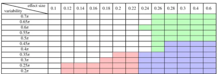
Secondly, in order to easily depict the compared behaviors of G-MVPA and ISPA, we overlapped the results of the two strategies into Table 3. In this third table, the blue cells in-dicate that NG > 50 and NI > 50 (i.e. that both G-MVPA

and ISPA produce significant results in more than half of the 100 datasets), while the green and red regions contain cells where it is the case only for G-MVPA or ISPA respectively (i.e. NG > 50 and NI < 50 in green cells; NI > 50 and

NG< 50 in red cells). Note that for completeness, we also used

different values of this arbitrary threshold set at 50, which did not qualitatively change the nature of the results described be-low (hence these results are not shown). We observe a large blue region in which both strategies provide concordant de-tections, for the largest values of the effect size d and with

(7)

Table 1: Number of datasets NG (out of 100) for which G-MVPA provides significant group decoding (in green: cells where NG≥ 50) variability e_{ffect size} 0.1 0.12 0.14 0.16 0.18 0.2 0.22 0.24 0.26 0.28 0.3 0.4 0.6 0.7π 7 11 15 22 27 36 40 44 53 59 68 96 100 0.65π 9 14 16 23 29 36 39 45 55 63 70 98 100 0.6π 13 16 17 25 27 35 44 53 58 71 76 95 100 0.55π 10 14 17 21 25 32 37 46 50 61 76 96 100 0.5π 7 8 15 17 22 30 36 46 55 59 64 94 100 0.45π 4 7 13 14 22 32 39 46 51 62 69 96 100 0.4π 8 11 18 22 26 31 40 49 54 63 72 97 100 0.35π 4 7 15 24 34 37 46 51 61 61 68 96 100 0.3π 10 14 24 26 31 40 46 57 58 71 78 95 100 0.25π 9 13 20 25 32 43 45 53 60 62 69 94 100 0.2π 9 12 15 19 28 34 39 50 59 67 75 95 100

Table 2: Number of datasets NI(out of 100) for which ISPA provides significant group decoding (in red: cells where NI ≥ 50)

variability effect size 0.1 0.12 0.14 0.16 0.18 0.2 0.22 0.24 0.26 0.28 0.3 0.4 0.6 0.7π 8 8 9 10 11 10 10 10 8 10 10 9 13 0.65π 5 8 8 8 9 10 9 10 14 14 14 13 19 0.6π 8 13 12 13 15 15 14 17 16 18 20 20 21 0.55π 13 13 14 15 20 19 23 22 25 26 26 25 27 0.5π 16 15 16 22 24 24 28 27 29 29 30 38 45 0.45π 19 21 22 26 29 32 34 42 47 53 53 59 67 0.4π 22 28 33 34 39 41 42 49 49 50 54 69 85 0.35π 21 27 32 37 44 50 55 61 68 69 74 85 93 0.3π 25 30 39 46 60 67 70 74 82 83 90 98 99 0.25π 44 56 63 69 73 79 84 90 94 96 96 100 100 0.2π 42 55 63 71 80 86 91 93 94 98 98 100 100

Table 3: Visual comparison of G-MVPA vs. ISPA (in blue: cells where both NG≥ 50 and NI ≥ 50; in green: cells where NG≥ 50

and NI < 50; in red: cells where NG< 50 and NI ≥ 50). variability effect size 0.1 0.12 0.14 0.16 0.18 0.2 0.22 0.24 0.26 0.28 0.3 0.4 0.6 0.7π 0.65π 0.6π 0.55π 0.5π 0.45π 0.4π 0.35π 0.3π 0.25π 0.2π

a moderately low amount of inter-individual variability. In-terestingly, the green and red regions, where one strategy de-tects a group-level effect while the other does not, also take an important area in the portion of the parameter space that was browsed by our experiments, which means that the two strate-gies can disagree. G-MVPA can provide a positive detection when the inter-individual variability is very large, while ISPA cannot (green region). But ISPA is the only strategy that of-fers a positive detection for very small effect sizes, requiring a moderate inter-individual variability (red region).

3.2. Results for fMRI datasets 3.2.1. Qualitative observations

For our two real datasets, the literature provides clear ex-pectations about brain areas involved in the tasks performed by the participants and the associated decoding question addressed in our experiments. The active finger movements performed by

the participants during the acquisition of Dataset1 are known to recruit contralateral primary motor and sensory as well as sec-ondary sensory cortices, ipsilateral dorsal cerebellum as well as the medial supplementary motor area [25]. In Dataset2, the participants were passively listening to vocal and non-vocal sounds. The contrast, or decoding, of these two types of stimuli is classically used to detect the so-called temporal voice areas, which are located along the superior temporal cortex (see e.g. [29]). We now describe the results obtained with G-MVPA and ISPA with respect to this priori knowledge.

The searchlight decoding analyses performed at the group level were all able to detect clusters of voxels where the de-coding performance was significantly above chance level (p < 0.05, FWE-corrected using permutation tests) with both G-MVPA and ISPA, for Dataset1 and Dataset2 and with all sizes of the spherical searchlight. The detected clusters were overall con-sistent across values of the searchlight radius, with an increas-ing size of each cluster when the radius increases. In Dataset1,

(8)

both strategies uncovered two large significant clusters located symmetrically in the left and right motor cortex. Additionally, ISPA was able to detect other significant regions located bilat-erally in the dorsal part of the cerebellum and the parietal oper-culum, as well as a medial cluster in the supplementary motor area (note that some of these smaller clusters also become sig-nificant with G-MVPA with the larger searchlight radii). These areas were indeed expected to be involved bilaterally given that button presses were given with both hands in this experiment. In Dataset2, both G-MVPA and ISPA yielded two large signif-icant clusters in the temporal lobe in the left and right hemi-spheres, which include the primary auditory cortex as well as higher level auditory regions located along the superior tem-poral cortices, matching the known locations of the temtem-poral voice areas. Figure 3 provides a representative illustration of these results, for a radius of 6 mm.

Figure 3: Illustration of the results of the group-level search-light decoding analysis for a 6 mm radius. Top two rows: Dataset1; bottom two rows: Dataset2. Brain regions found significant using G-MVPA and ISPA are depicted in green and red, respectively. A: primary motor and sensory cortices B:ipsilateral dorsal cerebellum C: medial supplementary motor area D: secondary sensory cortices E: superior temporal cortex

3.2.2. Quantitative evaluation

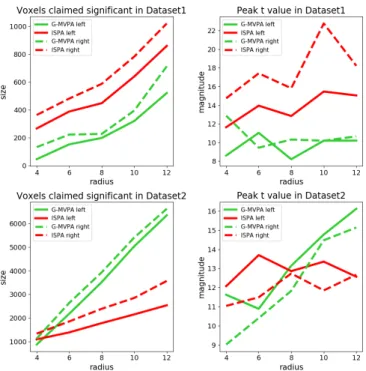
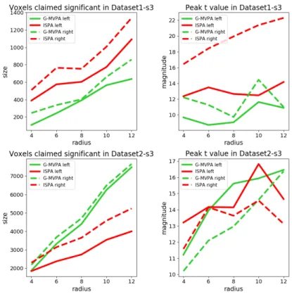
Our quantitative evaluation focuses on the two largest clus-ters uncovered in each dataset, i.e. the ones in the motor cortex for Dataset1 and the ones in the temporal lobe for Dataset2.

We first examine the size of these clusters, separately for each hemisphere and each of the five values of the searchlight ra-dius. The results are displayed in the left column of Figure 4. In almost all cases, the size of the significant clusters increased with the searchlight radius (left column). Moreover, the clus-ter located in the right hemisphere is consistently larger than the one on the left. In Dataset1, the cluster detected by ISPA is larger than the one detected by G-MVPA, regardless of the hemisphere, while in Dataset2, it is G-MVPA that yields larger clusters (except for a 4 mm radius where the sizes are similar). Then, we study the peak value of the t statistic obtained in each cluster (right column of Figure 4). In Dataset1, the peak t value is higher for ISPA than G-MVPA, for all values of the radius. In Dataset2, ISPA yields higher peak t values than G-MVPA for the searchlight radii smaller or equal than 8 mm, and lower peak t values for the larger radius values.

Figure 4: Quantitative evaluation of the results obtained on the real fMRI datasets for G-MVPA (green curves) and ISPA (red curves). Solid and dashed lines for the largest cluster in the left and right hemispheres respectively. Left column: size of the significant clusters. Right column: peak t statistic. Top vs. bottom row: results for Dataset1 and Dataset2 respectively.

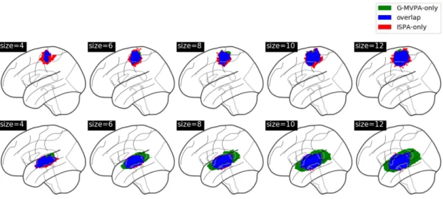
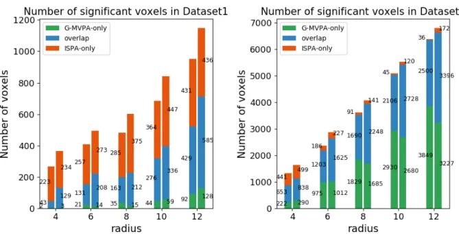
Then, we quantify the amount of overlap between the clus-ters found by G-MVPA and ISPA, by splitting the voxels into three sub-regions: voxels uncovered only by ISPA, only by G-MVPA or by both strategies (overlap). Figure 5 provides an illustration of these sub-regions, which shows that the overlap region (in blue) is located at the core of the detected clusters, while the voxels significant for only one strategy are located in the periphery; these peripheral voxels appear to be mostly detected by ISPA for Dataset1 (red voxels) and by G-MVPA for Dataset2 (green voxels). Figure 6 shows the voxel counts in

(9)

each sub-region, which confirms this visual inspection. Overall, the size of the sub-region found by the two strategies increases with the searchlight radius. The ISPA-only sub-region is larger in Dataset1 than in Dataset2, representing between 38% and 83% of all significant voxels. Conversely in Dataset2, the G-MVPA-only sub-region is more important – with a percentage of all significant voxels comprised between 18% and 60%.

We also count the number of voxels in each sub-region for each hemisphere. Figure 6 shows that for both datasets, the clusters in the right hemisphere are larger than in the left hemi-sphere. For both hemispheres, in most cases the number of voxels in each sub-region increases as the searchlight radius in-creases. However, in Dataset1, the number of voxels found only by G-MVPA is much smaller than that of overlap and ISPA-only sub-regions with all five radius values. In contrast, in Dataset2 the number of voxels in ISPA-only sub-regions de-creases for the four smallest values of the searchlight radius, and voxels only uncovered by ISPA are much fewer than those found only by G-MVPA.

4. Discussion

4.1. G-MVPA and ISPA provide different results

In this study, we have performed experiments on both real and artificial functional neuroimaging data in order to compare two group-level MVPA schemes that rely on classifier-based decoding analyses: the vastly used G-MVPA, and ISPA. Our results show that both strategies can offer equivalent results in some cases, i.e. that they both detect significant group-level multivariate effects in similar regions of the cortex for our two real fMRI datasets, and in parts of the two-dimensional param-eter space browsed using our artificially generated datasets, but that their outcomes can also differ significantly. For instance, in Dataset1, ISPA was the only strategy that detected multivariate group-level effects in several regions such as the supplementary motor area, the bilateral parietal operculum and dorsal cerebel-lum, for most of the searchlight radii that we tested (see an ex-ample on Figure 3 with a 6 mm radius). Furthermore, when a region is detected by both strategies, it usually differs in its size, extent and/or precise location, resulting in partial overlap; in most cases, the areas of concordance between the two strate-gies appeared to be centrally located, while the disagreements are located towards the periphery: in some areas, G-MVPA de-tects a group-level effect while ISPA does not, and inversely in other areas. Note that for Dataset2, our results generalize some of the observations reported in [13] with a different, yet compa-rable, framework of analysis, on a closely related data set.

Surprisingly, the peripheral behaviors were not consistent across the two real fMRI datasets: on Dataset1, ISPA only was able to detect effects on the periphery of the core region where both strategies were equally effective, while on Dataset2, it was G-MVPA which provided significant results on the pe-riphery. The results of the experiments conducted on the ar-tificial datasets can actually shed some light on these results, thanks to the clear dissociation that was observed in the two-dimensional parameter space browsed to control the properties

of the data. Indeed, ISPA is the only strategy that allows detect-ing smaller multivariate effects when the inter-individual vari-ability remains moderate, which is the case in the largest re-gions detected in Dataset1 because they are located in the pri-mary motor cortex, the pripri-mary nature of this region limiting the amount of inter-subject variability. On the opposite, the pe-ripheral parts of the temporal region detected in Dataset2 are lo-cated anteriorly and posteriorly to the primary auditory cortex, towards higher-level auditory areas where the inter-individual variability is higher, a situation in which G-MVPA revealed more effective in the experiments conducted with our artificial data.

4.2. ISPA: larger training sets improve detection power Our experiments revealed a very important feature offered by the ISPA strategy: its ability to detect smaller multivariate effects. On the one hand, this greater detection power was ex-plicitly demonstrated through the simulations performed on ar-tificial data, where the multivariate effect size was one of the two parameters that governed the generation of the data; we showed that with an equal amount of inter-individual variabil-ity, ISPA was able to detect effects as small as half of what can be detected by G-MVPA. Furthermore, on both real fMRI datasets, ISPA was able to detect significant voxels that were not detected using G-MVPA, in a large amount in Dataset1, and to a lesser extent in Dataset2. This detection power advantage is of great importance, since detecting weak distributed effects was one of the original motivations for the use of MVPA [15].

This greater detection power of ISPA is in fact the result of the larger size of the training set available: indeed, when the number of training examples is small, the performance of a model overall increases with the size of the training set, until an asymptote that is reached with large training sets – as encoun-tered in computer vision problems where millions of images are available from e.g. ImageNet6_{. In the case of functional}

neu-roimaging where an observation usually corresponds to an ex-perimental trial, we usually have a few dozen to a few hundred samples per subject, which clearly belongs to the small sample sizeregime, i.e. very far from the asymptote. In this context, ISPA offers the advantage to multiply the number of training samples by a factor equal to the number of subjects in the train-ing set, which is of great value. However, here, the increased sample size comes at the price of a larger heterogeneity in the training set, because of the differences that can exist between data points recorded in different subjects. If these differences are too large, they can represent an obstacle for learning, but if more moderate, the inter-subject variability can reveal ben-eficial by increasing the diversity of the training set. The fact that we observe a higher detection power with ISPA than with G-MVPA suggests that we are in the latter situation.

4.3. ISPA offers straightforward interpretation

When using the ISPA strategy, obtaining a positive result means that the model has learnt an implicit rule from the train-ing data that provides statistically significant generalization power

(10)

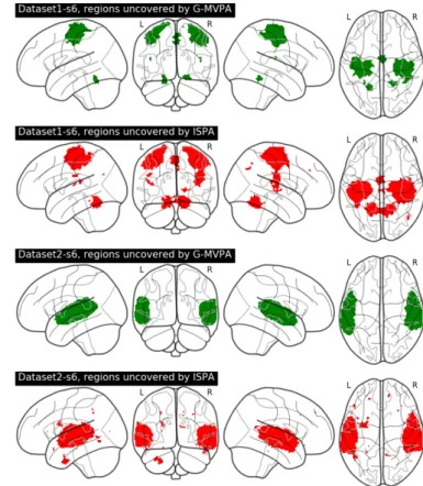
Figure 5: Comparison of the clusters detected by G-MVPA and ISPA for the different values of the searchlight radius, in Dataset1 (top row) and Dataset2 (bottom row).

on data from new subjects. Since a cross-validation of the type leave-one-subject-out or leave-n-subjects-out is performed on the available data to quantitatively assess such results, it allows to draw inference on the full population from which the group of participants was drawn, including individuals for which no data was available. As previously pointed out in [22], the inter-pretation that follows is straightforward: a significant effect de-tected with ISPA implies that some information has been iden-tified to be consistent throughout the full population. In more details, this means that the modulations of the multivariate pat-terns according to the experimental conditions that were the ob-ject of the decoding analysis are consistent throughout the pop-ulation, at least at the resolution offered by the modality used for the acquisition. This is the case for all voxels colored blue and red on Figure 5.

4.4. G-MVPA is more sensitive to idiosyncrasies

A significant result detected by G-MVPA but not ISPA – i.e. the green voxels on Figure 5, indicates that there is in-formation at the population level in the input patterns that can discriminate the different experimental conditions, but that the nature of the discriminant information present in the input vox-els differs across individuals. In other words, G-MVPA has detected idiosyncratic pattern modulations between conditions, which can be of great neuroscientific interest (see e.g. [7]), that could not have been identified with ISPA. This could be caused by two phenomenons. First, it could mean that the underlying coding strategy is nonetheless invariant across individuals, but that the nature of the data or of the feature space used in this analysis does not allow to identify it as such, e.g. because of an unperfect inter-subject registration of the functional maps. One would then need to acquire additional data using a di ffer-ent modality ([8]) or to transform the feature space (e.g. us-ing methods such as [14], [32] or [11]) in order to attempt to make this invariance explicit. Secondly, it could also mean that the neural code is simply intrinsically different across subjects,

for instance because several strategies had been employed by different individuals to achieve the same task, or because each subject employs its own idiosyncratic neural code. G-MVPA therefore only provides part of the answer, which makes the interpretation much less direct.

Note that beyond searchlight analyses, this potential ambi-guity could also occur with decoding performed in pre-defined regions of interest. Although such ROI-based decoding are vastly analysed at the group level using G-MVPA, numerous papers interpret the results as if G-MVPA allows identifying population-wise common coding principles, which cannot be claimed with only G-MVPA. These limitations have been pointed out previously in the literature, as in e.g. [33], [2] or [13], and we feel that the community should tackle this question more firmly. This could start by defining what a group-level multi-variate analysis should seek – a consistent amount or nature of the information. Finally, because G-MVPA and ISPA are some-how complementary, one could think about using both types of analysis to better assess neural coding principles.

4.5. A computational perspective

Finally, we examine here some practical considerations that are important for the practitioner, by comparing the computa-tional cost of G-MVPA and ISPA, and the availability of ready-to-use software implementations.

To assess the computational complexity of the two approaches, we first compare the number of classifiers that need to be trained for a full group analysis. Using G-MVPA, we need to train K classifiers per subject, where K is the chosen number of within-subject cross-validation folds, so KS classifiers in to-tal (where S is the number of available subjects). For ISPA, the number of cross-validation folds equals to S (for leave-one-subject-out), meaning we need to train a total of S classifiers. The training time of a classifier also depends on the number of training examples: it is linear for classifiers such as logis-tic regression (when using gradient-based optimizers [3]), and

(11)

Figure 6: Comparison of the voxel counts detected by G-MVPA-only (green), ISPA-only (red) or both (blue) for the different values of the searchlight radius, in Dataset1 (left) and Dataset2 (right).

quadratic for e.g. support vector machines [4]. Assuming we have n examples per subject, the number of training examples available for each classifier is (K−1)n_K for G-MVPA and (S − 1)n for ISPA. Overall, with linear-time classifiers, the total com-plexity of a group-level decoding analysis amounts to O(nKS ) for G-MVPA and O(nS2_{) for ISPA, which makes them almost}

equivalent if one assumes that K and S are of the same order of magnitude. With quadratic-time classifiers, the total com-plexity is O(n2KS) for G-MVPA and O(n2S3) for ISPA, which makes ISPA significantly more costly. We therefore advice to use linear-time classifiers such as logistic regression to perform ISPA analyses, particularly with searchlight decoding where the computational cost is further multiplied by the number of vox-els. Furthermore, note that thanks to its hierarchical nature, G-MVPA can be performed in an incremental manner for a low computational cost as participants get scanned: every time data from a new subject becomes available during the acquisition campaign, it suffices to run within-subject decoding for this new subject, which costs O(nK), plus the statistical test. This offers more flexibility for the experimenter than with the inter-subject scheme, for which performing IPSA every time a new subject is scanned amounts to re-doing a full analysis on all the subjects.

In terms of software implementation, because within-subject analyses have been the standard since the advent of MVPA, all software packages provide well documented examples for such analyses which are the base tool for G-MVPA. Even if it is not the case for ISPA, it is easy to obtain an equivalent implemen-tation because to perform inter-subject decoding, one simply need to i) have access to the data from all subjects, and ii) set up a leave-one-subject-out cross-validation, these two opera-tions being available in all software packages. As an example, we provide the code to perform ISPA searchlight decoding from

pre-processed data available online, which allows reproducing the results described in the present paper on Dataset2:

http://www.github.com/SylvainTakerkart/inter_subject_ pattern_analysis.

5. Conclusion

In this paper, we have compared two strategies that allow performing group-level decoding-based multivariate pattern anal-ysis of task-based functional neuroimaging experiments: the first is the standard method that aggregates within-subject de-coding results and a second one that directly seeks to decode neural patterns at the group level in an inter-subject scheme. Both strategies revealed effective but they only provide par-tially concordant results. Inter-subject pattern analysis offers a higher detection power to detect weak distributed effects and facilitate the interpretation while the results provided by the hi-erarchical approach necessitate further investigation to raise po-tential ambiguities. Furthermore, because it allows identifying group-wise invariants from functional neuroimaging patterns, inter-subject pattern analysis is a tool of choice to identify neu-romarkers [12] or brain signatures [22], making it a versatile scheme for population-wise multivariate analyses.

Acknowledgments

This work was carried out within the Institut Convergence ILCB (ANR-16-CONV-0002). It was granted access to the HPC resources of Aix-Marseille Universit´e financed by the project Equip@Meso (ANR-10-EQPX-29-01) of the French program Investissements d’Avenir. The acquisition of the data was made

(12)

possible thanks to the infrastructure France Life Imaging (11-INBS-0006) of the French program Investissements d’Avenir, as well as specific grants from the Templeton Foundation (40463) and the Agence Nationale de la Recherche (ANR-15-CE23-0026).

References

[1] Aglieri, V., Cagna, B., Belin, P., Takerkart, S., 2019. InterTVA. A mul-timodal MRI dataset for the study of inter-individual differences in voice perception and identification. OpenNeuro URL: https://openneuro. org/datasets/ds001771.

[2] Allefeld, C., Grgen, K., Haynes, J.D., 2016. Valid population infer-ence for information-based imaging: From the second-level t -test to prevalence inference. NeuroImage 141, 378–392. doi:10.1016/j. neuroimage.2016.07.040.

[3] Bach, F., 2014. Adaptivity of averaged stochastic gradient descent to local strong convexity for logistic regression. The Journal of Machine Learning Research 15, 595–627.

[4] Bottou, L., Lin, C.J., 2007. Support vector machine solvers. Large scale kernel machines 3, 301–320.

[5] Brodersen, K.H., Daunizeau, J., Mathys, C., Chumbley, J.R., Buh-mann, J.M., Stephan, K.E., 2013. Variational Bayesian mixed-effects inference for classification studies. NeuroImage 76, 345– 361. URL: https://linkinghub.elsevier.com/retrieve/pii/ S1053811913002371, doi:10.1016/j.neuroimage.2013.03.008. [6] Capilla, A., Belin, P., Gross, J., 2012. The Early Spatio-Temporal

Corre-lates and Task Independence of Cerebral Voice Processing Studied with MEG. Cerebral Cortex 23, 1388–1395. doi:10.1093/cercor/bhs119. [7] Charest, I., Kievit, R.A., Schmitz, T.W., Deca, D., Kriegeskorte, N., 2014. Unique semantic space in the brain of each beholder predicts perceived similarity. Proceedings of the National Academy of Sciences 111, 14565– 14570. doi:10.1073/pnas.1402594111.

[8] Dubois, J., de Berker, A.O., Tsao, D.Y., 2015. Single-Unit Recordings in the Macaque Face Patch System Reveal Limit ations of fMRI MVPA. Journal of Neuroscience 35, 2791–2802. doi:10.1523/JNEUROSCI. 4037-14.2015.

[9] Etzel, J.A., 2015. MVPA Permutation Schemes: Permutation Testing for the Group Level, in: 2015 International Workshop on Pattern Recognition in NeuroImaging, pp. 65–68. doi:10.1109/PRNI.2015.29.

[10] Etzel, J.A., Valchev, N., Gazzola, V., Keysers, C., 2016. Is brain activ-ity during action observation modulated by the perceived fairness of the actor? PLoS One 11, e0145350.

[11] Fuchigami, T., Shikauchi, Y., Nakae, K., Shikauchi, M., Ogawa, T., Ishii, S., 2018. Zero-shot fMRI decoding with three-dimensional registration based on diffusion tensor imaging. Scientific Reports 8. doi:10.1038/ s41598-018-30676-3.

[12] Gabrieli, J., Ghosh, S., Whitfield-Gabrieli, S., 2015. Prediction as a Hu-manitarian and Pragmatic Contribution from Human Cogniti ve Neuro-science. Neuron 85, 11–26. URL: http://linkinghub.elsevier. com/retrieve/pii/S0896627314009672, doi:10.1016/j.neuron. 2014.10.047.

[13] Gilron, R., Rosenblatt, J., Koyejo, O., Poldrack, R.A., Mukamel, R., 2017. What’s in a pattern? examining the type of signal multivariate analysis uncovers at the group level. NeuroImage 146, 113–120. [14] Haxby, J., Guntupalli, J., Connolly, A., Halchenko, Y., Conroy, B.,

Gob-bini, M., Hanke, M., Ra madge, P., 2011. A Common, High-Dimensional Model of the Representational Space in Human Ventral Temporal Cortex. Neuron 72, 404–416. doi:10.1016/j.neuron.2011.08.026. [15] Haxby, J.V., Connolly, A.C., Guntupalli, J.S., 2014.

Decod-ing Neural Representational Spaces Using Multivariate Pattern Analysis. Annual Review of Neuroscience 37, 435–456. URL: http://dx.doi.org/10.1146/annurev-neuro-062012-170325, doi:10.1146/annurev-neuro-062012-170325.

[16] Haxby, J.V., Gobbini, M.I., Furey, M.L., Ishai, A., Schouten, J.L., Pietrini, P., 2001. Distributed and Overlapping Representations of Faces and Ob-jects in Ventral Temporal Cortex. Science 293, 2425–2430.

[17] Helfinstein, S.M., Schonberg, T., Congdon, E., Karlsgodt, K.H., Mum-ford, J.A., Sabb, F.W., Cannon, T.D., London, E.D., Bilder, R.M.,

Pol-drack, R.A., 2014. Predicting risky choices from brain activity patterns. Proceedings of the National Academy of Sciences 111, 2470–2475. [18] Izuma, K., Shibata, K., Matsumoto, K., Adolphs, R., 2017. Neural

pre-dictors of evaluative attitudes toward celebrities. Social cognitive and affective neuroscience 12, 382–390.

[19] Jiang, J., Summerfield, C., Egner, T., 2016. Visual Prediction Error Spreads Across Object Features in Human Visual Cortex. The Journal of Neuroscience 36, 12746–12763. doi:10.1523/JNEUROSCI.1546-16. 2016.

[20] Kim, J., Wang, J., Wedell, D.H., Shinkareva, S.V., 2016. Identifying core affect in individuals from fmri responses to dynamic naturalistic audiovi-sual stimuli. PloS one 11, e0161589.

[21] Koechlin, E., Jubault, T., 2006. Broca’s Area and the Hi-erarchical Organization of Human Behavior. Neuron 50, 963– 974. URL: https://linkinghub.elsevier.com/retrieve/pii/ S0896627306004053, doi:10.1016/j.neuron.2006.05.017. [22] Kragel, P.A., Koban, L., Barrett, L.F., Wager, T.D., 2018. Representation,

Pattern Information, and Brain Signatures: From Neurons to Neuroimag-ing. Neuron 99, 257–273. URL: https://linkinghub.elsevier. com/retrieve/pii/S089662731830477X, doi:10.1016/j.neuron. 2018.06.009.

[23] Kriegeskorte, N., Goebel, R., Bandettini, P., 2006. Information-based functional brain mapping. Proceedings of the National Academy of Sci-ences 103, 3863–3868.

[24] Lindquist, M.A., Krishnan, A., Lpez-Sol, M., Jepma, M.e., Woo, C.W., Koban, L., Roy, M., Atlas, L.Y., Schmidt, L., Chang, L.J., Reynolds Losin, E.A., Eisenbarth, H., Ashar, Y.K., Delk, E., Wager, T.D., 2017. Group-regularized individual prediction: theory and application to pain. NeuroImage 145, 274–287. doi:10.1016/j.neuroimage.2015. 10.074.

[25] Mima, T., Sadato, N., Yazawa, S., Hanakawa, T., Fukuyama, H., Yonekura, Y., Shibasaki, H., 1999. Brain structures related to ac-tive and passive finger movements in man. Brain 122, 1989–1997. URL: https://academic.oup.com/brain/article-lookup/doi/ 10.1093/brain/122.10.1989, doi:10.1093/brain/122.10.1989. [26] Mumford, J.A., Turner, B.O., Ashby, F.G., Poldrack, R.A., 2012.

Decon-volving BOLD activation in event-related designs for multivoxel pattern classification analyses. NeuroImage 59, 2636–2643. doi:10.1016/j. neuroimage.2011.08.076.

[27] Nichols, T.E., Holmes, A.P., 2002. Nonparametric permutation tests for functional neuroimaging: a primer with examples. Human brain mapping 15, 1–25.

[28] Olivetti, E., Veeramachaneni, S., Nowakowska, E., 2012. Bayesian hy-pothesis testing for pattern discrimination in brain decoding. Pattern Recognition 45, 2075–2084. URL: https://linkinghub.elsevier. com/retrieve/pii/S0031320311001841, doi:10.1016/j.patcog. 2011.04.025.

[29] Pernet, C.R., McAleer, P., Latinus, M., Gorgolewski, K.J., Charest, I., Bestelmeyer, P.E., Watson, R.H., Fleming, D., Crabbe, F.a., Valdes-Sosa, M., et al., 2015. The human voice areas: Spatial organization and inter-individual variability in temporal and extra-temporal cortices. Neuroim-age 119, 164–174.

[30] Ryali, S., Supekar, K., Abrams, D.A., Menon, V., 2010. Sparse logistic regression for whole-brain classification of fmri data. NeuroImage 51, 752–764.

[31] Stelzer, J., Chen, Y., Turner, R., 2013. Statistical inference and multi-ple testing correction in classification-based multi-voxel pattern analysis (mvpa): random permutations and cluster size control. Neuroimage 65, 69–82.

[32] Takerkart, S., Auzias, G., Thirion, B., Ralaivola, L., 2014. Graph-based inter-subject pattern analysis of fMRI data. PloS ONE 9, e104586. doi:10.1371/journal.pone.0104586.

[33] Todd, M.T., Nystrom, L.E., Cohen, J.D., 2013. Confounds in multivariate pattern analysis: Theory and rule representation case study. NeuroIm-age 77, 157–165. doi:10.1016/j.neuroimNeuroIm-age.2013.03.039. bibtex: todd confounds 2013.

[34] Varoquaux, G., 2018. Cross-validation failure: Small sample sizes lead to large error bars. NeuroImage 180, 68–77. doi:10.1016/j. neuroimage.2017.06.061.

(13)

Inter-subject pattern analysis

A straightforward and powerful scheme for group-level MVPA

Qi Wang, Bastien Cagna, Thierry Chaminade, Sylvain Takerkart

https://doi.org/10.1016/j.neuroimage.2019.116205

Supplementary materials

1. Influence of the number of subjects and number of sam-ples per subject

Aim. Although the two real fMRI datasets used in our ex-periments have approximately the same total number of ob-servations (5400 obob-servations in Dataset1, 5616 obob-servations in Dataset2), they differ in the number of subjects that were scanned and the number of trials per subject: Dataset1 includes 360 trials for each of the 15 subjects, while Dataset2 offers 144 trials for 39 subjects. We here attempt to investigate whether this could explain some of the differences we observed in the results of G-MVPA and ISPA on these two datasets, using new artificial datasets.

Experiments. We therefore repeat the same set of experi-ments as in the paper, using new sets of 14300 datasets gener-ated to maintain the size of the training set constant and modu-lating the ratio between the number of subjects S and the num-ber of samples per subject N. We used the following parameter values: (S , N) ∈ {(9, 500), (11, 400), (17, 250), (21, 200), (51, 80), (101, 40), (201, 20), (401, 10)}, which allows maintain-ing the size of the group-level dataset approximately constant (and more particularly, the size of the ISPA training set is ex-actly constant at (S − 1) × N= 4000).

Results. We present below the results we obtained, under the same summarized form as in Table 3 of the paper. Tables S1 to S8 represent the two-dimensional parameter space spanned by d andΘ, for various values of the (S, N) couple. The cells colored in blue are those where G-MVPA and ISPA yielded sig-nificant group-level decoding for 50 or more datasets out of the 100, whereas in the green cells it is the case only for G-MVPA and in the red ones it is the case only for ISPA.

The shape of the region where G-MVPA yields 50 or more significant detections, corresponding here to the green and blue cells, remains approximately rectangular for all values of (S , N). But when the number of subject S increases, it is shifted to the right of the table, i.e. G-MVPA is effective only for larger ef-fect sizes. This is a direct consequence of the decreasing value of N, which is critical for within-subject decoding. For ISPA, the shape and location of the colored region (red and blue cells) where it is effective remains fairly constant, showing that ISPA

is not or weakly affected by the ratio N/S when the size of the training set is constant.

We now try to address the question of whether the difference in the N/S ratio between Dataset1 and Dataset2 can explain the fact that the most peripheral regions of the main clusters are detected by ISPA for Dataset1 and G-MVPA for Dataset2, in the light of the present results where we vary N/S in artificial datasets. The N/S ratio for Dataset1 is 360/15 = 24, while for Dataset2, it is 144/39 = 3.7. We reformulate the previous question as follows: if the N/S ratio of Dataset1 were smaller (i.e. closer to the one of Dataset2), could the peripheral voxels – which are red on Figure 5 of the paper, i.e. are detected by ISPA – become green, i.e. be detected only by G-MVPA? For this, consider a red cell in Table S3 (for which the N/S ratio is the closest to the one of Dataset1): can it become green when the ratio N/S decreases? We clearly see that it is not possible, i.e. that all red cells in Table S3 are also red (in almost all cases) in Tables S4 to S8 where N/S is smaller. We then ask the opposite question: if the N/S ratio of Dataset2 were larger (i.e. closer to the one of Dataset1), could the peripheral voxels – which are green on Figure 5 of the paper, i.e. are detected by G-MVPA – become red, i.e. be detected only by ISPA? For this, consider a green cell in Table S5 (for which the N/S ratio is the closest to the one of Dataset2): can it become red when the ratio N/S increases? We clearly see that it is not possible, i.e. that all green cells in Table S5 are also green (in almost all cases) in Tables S1 to S4 where the N/S ratio is larger. This parallel between the real and the artificial datasets therefore suggests that it is not the difference of N/S ratio between Dataset1 and Dataset2that can explain the different behaviors observed in the periphery of the significant clusters between G-MVPA and ISPA, illustrated on Figure 5 of the paper.

(14)

Table S1: Visual comparison of G-MVPA vs. ISPA, 9 subjects, 500 data points per subject

variability effect size _0.1 _0.12 _0.14 _0.16 _0.18 _0.2 _0.22 _0.24 _0.26 _0.28 _0.3 _0.4 _0.6 0.7π 0.65π 0.6π 0.55π 0.5π 0.45π 0.4π 0.35π 0.3π 0.25π 0.2π

Table S5: Visual comparison of G-MVPA vs. ISPA, 51 subjects, 80 data points per subject variability effect size _0.1 _0.12 _0.14 _0.16 _0.18 _0.2 _0.22 _0.24 _0.26 _0.28 _0.3 _0.4 _0.6 0.7π 0.65π 0.6π 0.55π 0.5π 0.45π 0.4π 0.35π 0.3π 0.25π 0.2π

(15)

2. Influence of the within-subject covariance

Aim. Group-level decoding is strongly influenced by the ratio of the inter- and withsubject variance. To study the in-fluence of this ratio, we performed experiments in the paper where the within-subject covarianceΣ was fixed and the inter-subject variability was parametrically controlled, using our gen-erative model to create a large number of artificial datasets. Here, we study whether our results hold when we change the within-subject variance.

Experiments. In this section we vary both the within- and inter-subject variability. We keep the same range of values for Θ, which controls the amount of inter-subject variability: Θ ∈ {0.2π, 0.25π, 0.3π, 0.35π, 0.4π, 0.45π, 0.5π, 0.55π, 0.6π, 0.65π, 0.7π}. And we generate five new sets of 14300 datasets using five values for the within-subject covariance matrix: Σ1= 1 0 0 5 ! , Σ2= 3 0 0 5 ! , Σ3= 5 0 0 5 ! , Σ4= 7 0 0 5 ! , Σ5 = 9 0 0 5 !

. We fix the number of subjects to 21 and generate 200 data points for each subject. Figure S1 illustrates the effect of each of these five covariance matrices on the properties of the generated datasets, for d = 2 and Θ = 0. In short, the distinctiveness of the two classes decreases fromΣ1toΣ5.

Figure S1: Illustration of the artificial datasets generated with five covariance matrices. Each line is a subpart of a single dataset (5 subjects shown amongst 21), d= 2 and Θ = 0.

Results. Our results are shown in Tables S9 to S13. As pre-viously, G-MVPA and ISPA yield more that 50 detections out of the 100 datasets available in each cell in regions that only partially overlap. Both strategies are strongly influenced by the within-subject covarianceΣ, i.e. they prove less effective when going fromΣ1 toΣ5, i.e. when the within-subject

distinctive-ness of the patterns decreases. However, the shape of the di ffer-ent regions in this parameter space remains constant: G-MVPA is effective in a rectangle area (blue + green cells), showing that it is not affected by the amount of inter-subject variability; and ISPA is effective in a triangle-like area (blue + red cells). This shows that the qualitative nature of our results does not seem to be affected by the value of Σ.

Table S9: Visual comparison of G-MVPA vs. ISPA,Σ1

(16)

3. Influence of spatial smoothing on the results obtained on the real fMRI datasets

Aim. The preprocessing steps performed in the paper on the two fMRI datasets did not include any spatial smoothing. Since there is a debate in the literature on the validity and interest of such smoothing when performing MVPA, we here study the influence of the smoothing on our results.

Experiments. We replicate the same experiments as in the paper by adding some spatial smoothing on the beta maps that are used to construct the inputs of the classifier. We use the Gaussian kernel implemented in SPM to perform the smoo-thing, with full-width at half-maximum values of 3 mm and 6 mm.

Results. For clarity, we denote as Dataset1-s3 and Dataset2-s3 the versions of the two datasets with the 3 mm smoothing, and Dataset1-s6 and Dataset2-s6 with the 6 mm smoothing. The results are presented in the same way as in the paper for the unsmoothed data: Figure S2 and S3 show the thresholded statistical maps, displaying the significant clusters; Figure S4 and S5 present the analysis of the size of the main cluster and its peak statistic value, for each dataset, each hemisphere and each size of the searchlight radius; finally, Figure S6 and S7 de-scribe how the main clusters obtained with G-MVPA and ISPA overlap.

Overall, the results obtained with smoothing are consistent with what we found with the unsmoothed data: clusters were found in the same regions of the brain, their size increased with the value of the searchlight radius and the patterns of overlap between the clusters found by G-MVPA and ISPA were overall similar.

The main effect of smoothing appears to be that the number of significant voxels increases when the size of the smoothing kernel increases, from 0 mm to 3 mm to 6 mm. This can be explained by the fact that a small amount of smoothing helps reduce noise which can slightly improve decoding accuracies on the one hand and also increase the reproducibility across cross-validation folds on the other hand. This therefore facili-tates detection as probed by our statistical test on accuracies.

Furthermore, a notable difference observed with 6 mm smoo-thing is the fact that the size of the activated clusters found by ISPA for Dataset2-s6 is as large as the ones found by G-MVPA, which is not the case with smaller or no smoothing (see bottom-left graph in Figure S5, compared with the one in Figure S4 or with Figure 4 in the paper). Congruently, the pattern of overlap-ping of the clusters found by the two strategies is modified for Dataset2-s6when compared with the one found with smaller or no smoothing (see the right graph of Figure S7, compared to the right graph on Figure S6 and Figure 6 in the paper): the number of voxels detected only by G-MVPA (green voxels) decreased in an important proportion. This is consistent with the puta-tive explanation that was put forward in the paper, that stated that the large amount of green voxels found in Dataset2 could be caused by a large inter-individual variability: indeed, one of the effect of spatial smoothing is often to reduce this inter-individual variability. In a complementary manner, this could also mean that the idiosyncrasies that could drive the detection

of the green voxels leave at high spatial frequencies. The spatial smoothing, by attenuating these frequencies, would therefore make them vanish as we observe in this experiment.

(17)

Figure S2: Illustration of the results of the group-level searchlight decoding analysis for a 6 mm radius with Dataset1-s3 and Dataset2-s3. Top two rows: Dataset1-s3; bottom two rows: Dataset2-s3. Brain regions found significant using G-MVPA and ISPA are respectively depicted in green and red.

Figure S3: Illustration of the results of the group-level searchlight decoding analysis for a 6 mm radius with Dataset1-s6 and Dataset2-s6. Top two rows: Dataset1-s6; bottom two rows: Dataset2-s6. Brain regions found significant using G-MVPA and ISPA are respectively depicted in green and red.

(18)

Figure S4: Quantitative evaluation of the results obtained on the smoothed fMRI datasets for G-MVPA (green curves) and ISPA (red curves), 3 mm Gaussian kernel. Solid and dashed lines for the largest cluster respectively in the left and right hemispheres. Left column: size of the significant clusters. Right column: peak

tstatistic. Top vs. bottom row: results for Dataset1-s3 and Dataset2-s3 respectively.

Figure S5: Quantitative evaluation of the results obtained on the smoothed fMRI datasets for G-MVPA (green curves) and ISPA (red curves), 6 mm Gaussian kernel. Solid and dashed lines for the largest cluster respectively in the left and right hemispheres. Left column: size of the significant clusters. Right column: peak

(19)

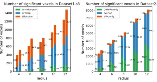
Figure S6: Comparison of the voxel counts detected by G-MVPA-only (green), ISPA-only (red) or both (blue) for the different values of the searchlight radius, in Dataset1-s3(left) and Dataset2-s3 (right)

Figure S7: Comparison of the voxel counts detected by G-MVPA-only (green), ISPA-only (red) or both (blue) for the different values of the searchlight radius, in Dataset1-s6(left) and Dataset2-s6 (right).