HAL Id: tel-01331790
https://tel.archives-ouvertes.fr/tel-01331790
Submitted on 14 Jun 2016
HAL is a multi-disciplinary open access
archive for the deposit and dissemination of sci-entific research documents, whether they are pub-lished or not. The documents may come from teaching and research institutions in France or abroad, or from public or private research centers.
L’archive ouverte pluridisciplinaire HAL, est destinée au dépôt et à la diffusion de documents scientifiques de niveau recherche, publiés ou non, émanant des établissements d’enseignement et de recherche français ou étrangers, des laboratoires publics ou privés.
Energy Characterization and Savings in Single and
Multiprocessor Systems : understanding how much can
be saved and how to achieve it in modern systems
Nicolas Triquenaux
To cite this version:
Nicolas Triquenaux. Energy Characterization and Savings in Single and Multiprocessor Systems : understanding how much can be saved and how to achieve it in modern systems. Distributed, Parallel, and Cluster Computing [cs.DC]. Université de Versailles-Saint Quentin en Yvelines, 2015. English. �NNT : 2015VERS042V�. �tel-01331790�
Université de Versailles Saint-Quentin-en-Yvelines École Doctorale "STV"
Étude et sauvegarde de la consommation
énergétique dans un environnement simple et
multi processeurs : Comprendre combien peut
être sauvegardé et comment y arriver sur des
systèmes modernes
Energy Characterization and Savings in Single and Multiprocessor Systems :
Understanding how much can be saved and how to achieve it in modern systems
THÈSE
présentée et soutenue publiquement le 18 Septembre 2015 pour l’obtention du
Doctorat de l’université de Versailles Saint-Quentin-en-Yvelines
(spécialité informatique) par
Nicolas Triquenaux
Composition du jury
Directeur de thèse : William JALBY - Professeur, Université de Versailles
Président : Claude TIMSIT - Professeur Emérite, Université de Versailles Rapporteurs : Christine EISENBEIS - Directeur de Recherche, INRIA
Philippe CLAUSS - Professeur, Université de Strasbourg Examinateurs : Pierre VIGNERAS - Ingénieur de Recherche, ATOS
Remerciements
Comme le dira chaque doctorant, il est facile de savoir quand une thèse commence mais beaucoup moins quand elle va finir et quel chemin elle va nous faire emprunter. Me voilà au bout du chemin. « Et heureux qui comme Ulysse, a fait un beau voyage », je tiens à remercier tous ceux qui ont jalonné ce périple de leurs présences, conseils et bonne humeur.
Je tiens tout d’abord à remercier mon directeur de thèse, William Jalby, pour la confiance et la liberté qu’il m’a accordé tout au long de mes travaux de recherche.
Je remercie ensuite M. Jean-Christophe Beyler de m’avoir proposé de faire une thèse, certes de manière quelque peu insistante dès le début de mon stage de fin d’étude. Je ne regrette en rien d’avoir décidé de le faire. Ceci m’a permis de voir jusqu’où je pouvais aller. Je le remercie aussi de m’avoir poussé dans mes moments de doutes.
Un très grand merci à l’équipe énergie qui est née et morte avec moi. Sans eux, je me serais trouvé bien seul face à cette mer capricieuse et changeante qu’est la thèse. Je remercie Benoit Pradelle pour avoir repris le flambeau quand Jean-Christophe est parti découvrir de nouveaux horizons. Je remercie Amina Germouche pour son expertise en programmation linéaire et pour son entreprise d’import export de pâtisserie algérienne soignant tout vague à l’âme. Jean Philipe Halimi pour avoir partagé parfois des problèmes communs quand il a fallu étudier les processeurs xeon-phi d’Intel. Alexandre Laurent pour m’avoir aidé à concevoir les premières briques d’UtoPeak. Et à tous, pour avoir partagé de bon moments gastronomiques.
Je remercie les rapporteurs pour avoir eu la patience de relire ma thèse juste avant leurs vacances. Je suis reconnaissant à Claude Timsit d’avoir su me donner goût à la recherche au cours de mes années d’étude et de m’avoir introduit au vaste monde du calcul scientifique. Enfin je remercie Pierre Vigneras de m’avoir laissé le temps de lui présenter mes travaux autour d’un café et d’avoir accepté de faire parti du jury.
Je remercie Jean Thomas Acquaviva qui, bien que ne faisant plus partie du laboratoire, m’a aidé dans la constitution du jury de thèse et m’a poussé un peu lorsque je laissais le travail fourni chez DataDirect Networks prendre le pas sur la rédaction de ce présent manuscrit.
Je remercie aussi Vincent Palomares, compagnon d’infortune, avec qui j’ai partagé une traversé du Styx mouvementé durant de longues nuits après avoir payé à Charon notre droit de passage en formulaire administratif.
Je remercie aussi mon épouse d’avoir fait preuve d’une grande patience sur la fin de la rédaction. La thèse est une amante qui ne souffre d’être délaissée et « l’enfer n’a pas de furie comme une femme dédaignée » – William Congreve.
Enfin je remercie ma belle-mère pour avoir fourni une expertise sans faille tout au long de la rédaction retirant en bien des endroits mes maladresses orthographiques et syntaxiques. Et je remercie aussi mes parents qui ont permis que je ne sois qu’a 15 minutes de marche de la faculté de Versailles.
ii
iii
Résumé:
Bien que la consommation énergétique des processeurs a considérablement diminué, la demande pour des techniques visant à la réduire n’a jamais été aussi forte. En effet, la consommation énergétique des machines haute performance a crû proportionnellement à leurs accroissements en taille. Elle a atteint un tel niveau qu’elle doit être minimisée par tous les moyens.
Les processeurs actuels peuvent changer au vol leurs fréquences d’exécution. Utiliser une fréquence plus faible peut mener à une réduction de leurs consomma-tions énergétiques. Cette thèse recherche jusqu’à quel point cette fonctionnalité, appelé DVFS, peut favoriser cette réduction. Dans un premier temps, une analyse d’une machine simple est effectuée pour une meilleure compréhension des différents éléments consommateurs afin de focaliser les optimisations sur ces derniers.
La consommation d’un processeur dépend de l’application qui est exécutée. Une analyse des applications est donc effectuée pour mieux comprendre leurs impacts sur cette dernière. Basés sur cette étude, plusieurs outils visant à réduire cette consommation ont été créés. REST, adapte la fréquence d’exécution au regard du comportement de l’application. Le second, UtoPeak, calcule la réduction maximum que l’on peut attendre grâce au DVFS. Le dernier, FoREST, est créé pour cor-riger les défauts de REST et obtenir cette réduction maximum de la consommation énergétique.
Enfin, les applications scientifiques actuelles utilisent généralement plus d’un processeur pour leurs exécutions. Cette thèse présente aussi une première tentative de découverte de la borne inférieure sur la consommation énergétique dans ce nouvel environnement d’exécution.
Mots cléfs:
Caractérisation de puissance, Caractérisation d’énergie, Contrôle des ventilateurs, Contrôle dynamique de fréquences, Profilage dynamique, Applications parallèles, Consommation énergétique minimale
iv
Abstract:
Over the past decade, processors have drastically reduced their power con-sumption. With each new processor generation, new features enhancing the processor energy efficiency are added. However, the demand for energy reduction techniques has never been so high. Indeed, with the increasing size of high per-formance machines, their power and energy consumptions have grown accordingly. They have reached a point where they have to be reduced by all possible means.
Current processors allow an interesting feature, they can change their operating frequency at run-time. As granted by transistor physics, lower frequency means lower power consumption and hopefully, lower energy consumption. This thesis investigates to which extent this processor feature, called DVFS, can be used to save energy.
First, a simple machine is analyzed to have a complete understanding of the dif-ferent power consumers and where optimizations can be focused. It will be demon-strated that only fans and processors allow run-time energy optimizations. Between the two, the processor shows the highest consumption, therefore potentially exposing the higher potential for energy savings.
Second, the power consumption of a processor depends on the applications being executed. However, there are as many applications as problems to solve. The focus is then put on applications to understand their impacts on energy consumption. Based on the gathered insights, multiple tools targeting energy savings on a single processor are created. REST, the most naive, tries to adapt the processor state to the stress generated by the application, hoping for energy reduction. The second, UtoPeak, computes the maximum energy reduction one can expect for any tool using DVFS. It allows to evaluate the efficiency of such systems. The last one, FoREST, was created in order to correct all the flaws of REST and target maximum energy reduction.
Last, scientific applications generally need more than one processor to be exe-cuted in a decent time. The thesis also presents a first attempt to compute a lower bound in energy reduction when considering this new execution context.
Keywords:
Power characterization, Energy characterization, Fan control, Dynamic frequency scaling, Dynamic profiling, Parallel applications, Lowest energy consumption
Contents
1 Introduction 1
I Power and Energy Popularization 5
2 Introduction 7
3 Metrics 9
3.1 Single Machine . . . 9
3.2 Parallel Systems And Clusters . . . 9
4 Hard Drive and Memory Energy Consumption 11 4.1 RAM . . . 11 4.1.1 Power Consumers . . . 12 4.1.2 Possible Optimizations . . . 12 4.2 Disk . . . 13 4.2.1 Power Consumers . . . 13 4.2.2 Possible Optimizations . . . 14 5 Fans 15 5.1 State Of The Art . . . 15
5.2 Motivations . . . 16 5.3 Power Characterization . . . 17 5.3.1 Fan Power . . . 17 5.3.2 Power Leakage . . . 19 5.4 DFaCE . . . 23 5.4.1 Overview . . . 23 5.4.2 Hill-Climbing . . . 25 5.4.3 System Load . . . 27
5.4.4 Temperature Stability And Critical Heat . . . 28
5.4.5 Convergence Speed And Optimal Temperature . . . 29
5.5 Power Savings . . . 32
6 CPU And Its Environment 35 6.1 Processor Power Model . . . 35
6.2 Advanced Configuration and Power Interface (ACPI) . . . 36
6.2.1 OSPM States . . . 36
6.2.2 P-state, C-state and Multi-core Chip . . . 39
6.3 Micro-benchmarking Characterization . . . 41 6.3.1 Measurement Methodology . . . 41 6.3.2 Test Environment . . . 43 6.4 Memory . . . 44 6.5 Arithmetic . . . 46 6.5.1 Instruction Clustering . . . 47
vi Contents
7 Conclusion 53
II DVFS single chip 55
8 Introduction 57
8.1 Application Trends . . . 58
8.1.1 External Resources Boundness . . . 58
8.1.2 Compute Boundness . . . 59
8.1.3 Balanced Boundness . . . 61
8.2 Phase Detection . . . 62
8.2.1 Static Phase Detection . . . 62
8.2.2 Dynamic Phase Detection . . . 68
8.3 Dynamic Voltage Frequency Scaling Latency . . . 72
9 Runtime Energy Saving Technology (REST) 79 9.1 State of The Art . . . 79
9.2 General Presentation . . . 80
9.2.1 Dynamic Profiler . . . 81
9.2.2 Decision Makers . . . 83
9.3 The Cost of Energy Savings . . . 89
9.4 The More The Better ? . . . 93
10 UtoPeak 95 10.1 State of The Art . . . 95
10.2 Under the Hood . . . 96
10.2.1 The Necessity of Profiling . . . 97
10.2.2 Normalization and Prediction . . . 99
10.3 UtoPeak Assumptions . . . 101
10.3.1 Constant Number of Executed Instructions . . . 101
10.3.2 Frequency Switch Latency . . . 101
10.4 Prediction Versus Real World . . . 102
10.5 UtoPeak DVFS Potential . . . 105
10.6 UtoPeak Versus The World . . . 107
11 FoREST 109 11.1 State of The Art . . . 109
11.2 Motivation . . . 110
11.2.1 Power Ratio . . . 110
11.2.2 Continuous Frequency . . . 114
11.2.3 Multicore Processors . . . 117
11.2.4 Frequency Transition Overhead . . . 117
11.3 Overview . . . 118
11.3.1 Offline Power Measurement . . . 118
11.3.2 Frequency Evaluation . . . 119
11.3.3 Sequence Execution . . . 120
11.4 FoREST Versus the World . . . 121
11.4.1 Energy Gains . . . 121
11.4.2 Performance Degradation . . . 123
Contents vii
11.4.4 Energy saving mode . . . 125
12 Conclusion 127 III DVFS multi chip 129 13 Introduction 131 13.1 State of The Art . . . 131
13.2 Execution Context . . . 133
13.3 Problematic . . . 135
13.3.1 Application Constraint . . . 136
13.3.2 Hardware Constraints . . . 137
13.4 This is not UtoPeak you are looking for . . . 139
14 OUTREAch : One Utopeak To Rule Them All 141 14.1 Application Profiling . . . 141
14.2 Tasks And Communication Profiling . . . 143
14.3 Energy Normalization . . . 147
14.4 Building The Linear Program . . . 148
14.4.1 Precedence Constraints . . . 149
14.4.2 Execution Time Limitation . . . 151
14.4.3 Architecture Constraints: The Workload Approach . . . 152
14.4.4 Architecture Constraints: The Frequency Switch Date Approach156 14.4.5 Discussion . . . 158
14.4.6 Super Tasks . . . 159
14.5 Experimental Results . . . 160
14.6 OUTREAch versus the world . . . 164
14.7 What Next ? . . . 167
15 Conclusion 171 16 Conclusion 173 16.1 Contribution of This Thesis . . . 173
16.2 Future Works . . . 175
List of Figures
2.1 Power Profile for Several Workloads [44] . . . 8 4.1 General overview of DRAM device structure, extracted from [35] . . 12 5.1 Illustrating the balance between fan power consumption and powerleakage. . . 17 5.2 Power consumed by a standard 120mm CPU fan at different speeds. 18 5.3 Power consumption of a Intel Core i5 2380P processor at different
temperatures. . . 21 5.4 Normalized Power consumption of a Intel Core i5 2380P processor at
different temperatures. . . 22 5.5 Power leakage of a Intel Core i5 2380P processor at different
temper-atures. . . 24 5.6 Overview of the general system’s algorithm. . . 25 5.7 The optimizer evaluates several solutions while always progressing
toward the optimum. . . 26 5.8 Overview of the learning strategy. . . 26 5.9 DFaCE evaluates only a subset of the fan settings before converging
on the optimum. . . 30 5.10 Fan power consumption plus power leakage, and CPU temperature
converge towards the optimal solution with a 25% load level. . . 31 5.11 Fan power consumption plus power leakage, and CPU temperature
converge towards the optimal solution with an half-loaded CPU. . . 31 6.1 ACPI state tree. . . 37 6.2 Voltage and Frequency up-scaling/down-scaling behavior. . . 38 6.3 Kernel Assembly instructions . . . 44 6.4 Energy consumption per memory instruction depending on the data
location when the memory is saturated . . . 45 6.5 Energy consumption per memory instruction depending on the data
location when the memory is not saturated . . . 45 6.6 Micro-benchmark for arithmetic intensive execution . . . 46 6.7 Arithmetic instruction energy consumption on E3-1240 at 3.3GHz . . 47 6.8 Arithmetic instruction power consumption evolution on SandyBridge
E3-1240 . . . 49 6.9 Energy consumption of one instruction per class. . . 50 8.1 Data fetching latency from each cache level. . . 59 8.2 Wall energy consumption and time execution for the SPEC program
libquantum depending on frequencies. . . 60 8.3 Wall energy consumption and time execution for the SPEC program
gromacs depending on frequencies. . . 61 8.4 Wall energy consumption and time execution for the RTM program
depending on frequencies . . . 61 8.5 Execution time of each codelet of IS and the difference between the
x List of Figures 8.6 Execution time of each codelet of BT and the difference between the
re-calculated and the measured ones. . . 65
8.7 Energy consumption of each IS codelet and the difference between the re-calculated and the measured ones. . . 66
8.8 Energy consumption of each codelet of BT and the difference between the re-calculated one and the measured one. . . 67
8.10 Hardware counters during the execution of a synthetic benchmark: showing how the counters evolve between a memory bound and a compute bound execution . . . 71
8.11 Hardware counters during the execution of a real world application (RTM) . . . 72
8.12 Step before actual frequency switch . . . 73
8.13 Observed execution times of the assembly kernel for the pair (1.6 GHz, 3.4 GHz) of CPU frequencies on the IvyBridge machine . . . . 75
8.14 Latency to change frequency on an Westmere architecture . . . 76
8.15 Latency to change frequency on an SandyBridge architecture . . . . 76
8.16 Latency to change frequency on an IvyBridge architecture . . . 77
8.17 Frequency transition latency versus phase duration . . . 77
9.1 REST system overview . . . 80
9.2 Different profiler waking period . . . 82
9.3 Naïve frequency mapping . . . 84
9.4 Hardware counters during the execution of a real world application (RTM) . . . 85
9.5 Frequency confidence level evolution . . . 86
9.6 The Markovian Graph construction evolution . . . 87
9.7 REST energy savings and performance degradation on the SPEC 2006 benchmark suite, with the most naïve decision maker . . . 91
9.8 REST energy savings and performance degradation on the parallel NAS benchmarks using the naïve decision maker . . . 92
9.9 REST energy savings and performance degradation on the SPEC benchmarks using branch prediction decision maker . . . 93
9.10 Naïve decisions lead to better energy saving and lower performance slowdown on a subset of tested applications . . . 94
9.11 Branch prediction decisions lead to better energy saving and lower performance slowdown on a subset of tested applications . . . 94
10.1 UtoPeak’s general overview. . . 96
10.2 UtoPeak profiling information during IS execution at 1.6GHz. . . 97
10.3 Difference between time-based and instruction-based sampling. . . . 98
10.4 Normalized energy per instruction samples for GCC and POVRAY. 104 10.5 Energy consumption prediction error on GCC benchmark . . . 105
10.6 REST compared to UtoPeak . . . 108
11.1 Power consumption evolution for SPEC and NAS benchmarks pro-gram . . . 111
11.2 An example of a frequency pair and the associated IPS. . . 114
11.3 FoREST’s architecture overview. . . 118
11.4 Energy consumption normalized to that achieved by ondemand. 5% slowdown required for FoREST and beta-adaptive. . . 122
List of Figures xi 11.5 Execution time normalized to that achieved by ondemand. 5%
slow-down required for FoREST and beta-adaptive. . . 123
11.6 Forest frequency selection when running the is program with 5% slowdown. . . 124
11.7 Execution time normalized to that achieved by ondemand. 100% slow-down allowed for Forest and beta-adaptive. . . 125
11.8 Energy savings over what ondemand achieves. 100% slowdown allowed for Forest and beta-adaptive. . . 126
13.1 Parallel Application Tasks Abstraction. . . 134
13.2 Task graph . . . 134
13.3 Different execution scenario and their potential optimization . . . 136
13.4 Task optimization impact on overall graph . . . 137
13.5 Frequency shift constraint . . . 138
14.1 OUTREAch’s steps overview . . . 141
14.2 Task and communication timing . . . 142
14.3 Task dependencies . . . 143
14.4 OUTREAch Task profiling . . . 144
14.5 Task Graph Reconstruction . . . 145
14.6 Difference between time-based and instruction-based sampling. . . . 148
14.7 Slack time . . . 150
14.8 Workloads . . . 152
14.9 Workloads and tasks execution . . . 154
14.10Negative workload duration for impossible workloads . . . 155
14.11Frequency switches example . . . 158
14.12Task graph to super-task graph . . . 159
14.13Frequency shift constraint . . . 165
List of Tables
2.1 Computer Power Consumption Break-Down. . . 7
5.1 Power cost of using an extra processor core . . . 22
5.2 Optimal CPU temperature for different workload levels. . . 32
5.3 Power savings achieved by DFaCE compared to thermal-directed cooling with a target temperature of 50◦C or 60◦C. . . 33
6.1 Intel Pentium M at 1.6GHz P-state detail. . . 37
6.2 P-state and C-state usage while writing this PhD thesis. . . 39
6.3 ADDPS benchmark execution time for several consecutive executions. 42 6.4 Experimental Testbed. . . 43
6.5 Arithmetic instructions reciprocal throughput. . . 48
6.6 Arithmetic instructions power consumption . . . 48
8.1 BT and IS codelets overview . . . 63
8.2 BT Gprof condensed summary. . . 68
9.1 Valid frequency shift versus non valid ones . . . 88
9.2 Experimental Testbed . . . 90
10.1 Theoretical program sampling and normalization results . . . 99
10.2 Theroritical application’s frequency sequence. . . 100
10.3 UtoPeak energy guessing precision for SPEC2006 and NAS-OMP sorted by decreasing precision . . . 103
10.4 DVFS energy reduction potential for SPEC2006 and NAS-OMP sorted by increasing DVFS potential . . . 106
11.1 Example of power ratios for two frequencies across all SPEC and NAS benchmark programs . . . 113
11.2 Best Frequency Pair Generation variable definition . . . 115
11.3 Sample measurement results from offline profiling and online evalua-tion for one processor core . . . 119
11.4 FoREST energy savings compared to UtoPeak. . . 126
13.1 Energy consumption comparison between multiple UtoPeak and the best static frequency . . . 139
14.1 OUTREAch instrumentation impact . . . 146
14.2 Task variables . . . 149
14.3 Workload formulation variables . . . 153
14.4 Frequency switch formulation variables . . . 157
14.5 OUTREAch accuracy on NAS parallel benchmarks programs with two limit on performance degradation. . . 161
14.6 OUTREAch energy reduction potential . . . 163
14.7 OUTREAch converging time with and without the super-task graph compression . . . 164 14.8 Energy reduction potential comparison between OUTREAch and SC07.165
xiv List of Tables 14.9 Time to solution comparison between OUTREAch and SC07. . . 166
Chapter 1
Introduction
The concerns on energy consumption and its ecological impacts did not rose overnight. Some people say that there always was a sub-part of the society to worry about the ecological impacts of the skyrocketing needs in energy worldwide. Others would tell that no one really care about such concerns as long as there is profit. And more dramatically,a few rave that unless an imminent huge disaster hap-pens, every thing will remain unchanged because those who are wasting the most energy refuse to see its long term impacts. What is known, is that these concerns on energy consumption were publicly acknowledged during the first Earth Summit in 1972 along with many other ecological concerns. Following this Earth Summit, several treaties were issued to unit all the countries towards the same goal. During the second edition of the Earth summit, the United Nations Framework Convention on Climate Change (UNFCCC) was given birth. Signed by 165 countries, it is a framework for negotiating specific international treaties that may set binding limits on greenhouse gas. It helped designing the Kyoto protocol signed on December 11th 1997. From then, the interest in tackling the energy consumption issues as well as other ecological matters went snowballing.
In the world of High Performance Computing (HPC), the term "Performance" was until recently the preponderant criteria to evaluate how well an application is executed. However, with the ever growing demand for performance associated with a higher and higher complexity of the problems to be tackled, the size of HPC sys-tems dramatically increased along with their power consumption. As an example, the first machine on november top500 list, Tianhe-2 consumes 17 Mw. To power such a machine is not the sole problem, the machine has to be cooled down to pre-vent overheating. For example, 0.7W of cooling is needed to dissipate every 1W of power consumed by one HPC system at Lawrence Livermore National Labora-tory [131]. The data is a bit old, and the ratio surely has been enhanced, but still the amount of power to operate such gigantic machine is tremendous. And when looking at the overall picture, the growth will not stop. In 2013, U.S. data centers consumed an estimated 91 billion kilowatt-hours of electricity. This is the equivalent annual output of 34 large (500-megawatt) coal-fired power plants, enough electricity to power all the households in New York City twice over. Data center electricity con-sumption is projected to increase to roughly 140 billion kilowatt-hours annually by 2020, the equivalent annual output of 50 power plants, costing American businesses $13 billion per year in electricity bills and causing a yearly emission of nearly 150 million metric tons of carbon pollution [6]. Power and energy consumption can no longer be ignored and the energy consumption may replace the performance criteria to evaluate how well an application is executed.
Power and energy consumption have then to be optimized by any possible means. Dynamic Voltage Frequency Scaling (DVFS) was then selected as the flagship of that new crusade. As it will be seen later on, processors power scales quadratically to the voltage and linearly to the operating frequency. Moreover, coming from the transistor physics, the frequency and voltage are linked to eachother. Higher voltage
2 Chapter 1. Introduction allows to operate faster, and slower operations allow lower voltage. Then by lowering the operating frequency, tremendous energy consumption can be saved, roughly cubic to the processor frequency. By using that interesting property, a wide range of tools and techniques were built and all of them reported energy reductions. However, Le Sueur et. al. [100] well expose the problematic brought with the tremendous decrease in transistor miniaturization. With smaller transistors, the core voltage was drastically reduced, from 5V with 0.8µm transistor feature size to 1.1-1.4V when considering 32nm transistor size. After that assessment, the authors pretend that the potential to save energy via DVFS is dramatically reduced. However, processors efficiency was enhanced with each new generation. Current processors expose a wide range of frequencies, fifteen for the SandyBridge and IvyBridge processors used during this thesis compared to ten for an older Westmere architecture. A wider range of frequencies, allows a better control over the application execution, thus better tuning for energy reduction. Deeper sleep state also are exposed with each new processor generation. As an example on the fourth generation of Intel processors [79], the deepest sleep state allows entire cores to shut down. Moreover, the new Haswell architecture now embarks the voltage regulator on the die, allowing a more efficient power management [64]. A legitimate question then arise when facing all these processor energy efficiency enhancements : is DVFS still a legitimate technique to reduce processors energy consumption while being used ?
This thesis will bring an answer to this question. It will be shown that DVFS techniques, even though they have a limited impact on sequential application, have a huge potential for energy saving for parallel applications.
The first part presents a vulgarization on energy and power consumption. In order to demytify what power and energy consumption mean, different power con-sumers of a simple machine are analyzed. For each of them, possible optimization mechanics are presented. For the processor power consumption, a more in-depth study is performed to understand how it consumes power under different kind of pressure and what are the means to reduce to consume less.
The second part provides an in depth analysis of applications energy consump-tions. Even though the amount of energy is partially dictated by the hardware, the pressure the application puts on the processor and the time it takes to be executed also plays an important part. It will be demonstrated that an application can be seen as a sequence of different phases with different purposes and resource needs. By identifying each application phase, and adapting the processor operating frequency to each of them, the overall application energy consumption is reduced. One could see the application phases identification as the major challenge, however this thesis is not about finding the best phase identification algorithm but to match the processor speed to each application phase at best. Nevertheless, two different phase identifi-cation techniques are presented, either static or dynamic. It is demonstrated that the dynamic phase identification allows more flexibility and has less overhead than the static method for the purpose of the DVFS techniques presented thereafter. In total three different techniques are presented: REST, UtoPeak and FoREST. The first one, REST, is a first naive attempt to acknowledge if DVFS techniques are worth the effort. It shows that on various application execution set-ups more than 25% of their energy consumption can be saved. However, as for all the other DVFS based tool there is no clear view on which maximum level of improvement can be expected. To solve that, UtoPeak is created. It is a static tool accurately predicting for one application execution, the maximum energy reduction one can expect from
3 DVFS based tools. Though the impact of DVFS is limited on sequential applica-tions, it shows that, for parallel applicaapplica-tions, at most 45% of the application energy can be saved. Though UtoPeak is able to grant maximum energy reduction, it is static and needs multiple runs of the same application to gather enough informa-tion to produce a realistic predicinforma-tion. FoREST, is created to dynamically achieve the maximum energy saving uncovered by UtoPeak in one application execution. Since it is a dynamic tool, and HPC people are not yet ready to sacrifice too much performances on the altar of energy reduction, FoREST also takes into account a performance degradation limit. FoREST performs the maximum energy reduction regarding that limit. Finally, FoREST adaptivity was further extended to take into account the overall machine energy consumption, and adapt the processor frequency to minimize the overall consumption. It demonstrates that DVFS is good to reduce processor energy consumption, but it cannot be used alone to achieve full machine energy savings.
The previous part demonstrates that DVFS is legitimate when considering paral-lel applications on a single processor. However does this transpose to multi-processor environments? The last part expose the first elements of an answer. It presents a static tool that predicts the maximum energy saving one can expect for one appli-cation regarding its execution set-up and confirms also that DVFS is still legitimate even when considering multiple processors environment.
Part I
Chapter 2
Introduction
As introduced previously, it is costly to operate data centers and any energy con-sumption reduction can be translated in significant money saving. It explains the existence of various energy reduction mechanisms seen in the next Parts. However before designing systems that grant energy reduction, the energy consumption has to be understood by itself.
The term Energy can be found in multiple domains, like mechanics, nuclear power, or electricity and is always used as a rate of performing work over time. The energy is generally computed as : P × T where P is the rate of activity, and T the time slice on which the work is done. In electricity the power P , is generated by an electric current passing through an electric potential. As an analogy consider a watermill being the electric potential and the flow of water being the electric current. The higher the flow of water on the water wheel the higher the grind force. The watermill energy quantifies the grind force over the period of use. When considering a computer, electrical power is what is needed to operate it and energy is used to quantify the consumed power until it is shutdown. Though, the watermill or the computer have just been considered as a unique entities, it is their composing parts that define the overall needed power to activate them. For the watermill a certain level of power is required to rotate the water wheel and additional power to rotate the grind wheel. It is the same for a computer with the motherboard, memory dims, disks, fans and the processors each need a fraction of the overall computer power. As an example, Table 2.1 shows the power needs of the different computer parts. Each stated value are coming from components data sheet that can be found in any computer hardware resellers.
The values showed in Table 2.1 are the worst case power consumption. Depend-ing on the situation, each part can draw more or less power. Back to the watermill, the grind power will variate regarding meteorological factors. If huge waterfall hap-pened upstream, the water’s flow will grant more grind force. At the opposite, if a drought occur, the water’s flow will decrease, decreasing the grind force. It is the same for a computer, depending on the usage scenario each computer part will draw more or less power as shown in Figure 2.1.
Figure 2.1 extracted from [44] shows different usage scenario measured on a Be-Computer’s Parts Power Consumption Ratio in Percentage
Processor 80W 57.7 %
Mother Board 35W 25.1 %
Ram modules 6W 4.3 %
HDD 6W 4.3 %
Fans 12W 8.6 %
8 Chapter 2. Introduction 0.0 5.0 10.0 15.0 20.0 25.0 30.0 35.0 40.0
idle 171.swim 164.gzip cp scp
CPU Memory Disk NIC
Power Consumption Distribution for Different Workloads Note: only power consumed by CPU, memory, disk and NIC are considered here
Figure 2.1: Power Profile for Several Workloads [44]
owulf node machine. It can be seen that each component consumes a part of the overall machine power. They can drastically change their needs regarding the com-puter usage scenario. It can be acknowledged that in most scenarios the processor is the part with the highest consumption. However, disks and memory are not to be neglected since they can consume more than 50% of the overall power in the cp scenario.
In the end, the energy consumption can vary regarding the duration and re-garding different usage scenarios. Therefore it is essential to fully understand how each computer component consumes power. Relying on these insight, it is possible to determine the means to reduce these consumptions and design energy reduc-tion techniques. However, before jumping into further details, it is as important to understand why the energy criteria is only used in this thesis and not for example energy-delay or other metrics derived from it. Once it is clear that the energy is con-sidered as the baseline metric, the focus is put on each machine power consumer. Ram dimms and disk power consumption and optimization will be first studied. They do not represent a significant part of a single machine power consumption, however data centers do not use only a single disk and two ram dims, but many thousands, making them a non-negligible power consumer. The RAM dims and HDD study will be followed by the study of fans power consumptions and how these elements can prevent the processor from consuming more. It will also be seen in Chapter 5 that the fans are always operated at their maximum speed even when un-necessary , making them wasting power. Finally, in Chapter 6 the processor power consumption and the means to reduce it are presented. Unlike for RAM dims, HDD and fans, techniques to reduce the processor power consumption and energy are not presented in the chapter since they are the purpose of the thesis.
Chapter 3
Metrics
Metrics are essential to quantify, measure, and evaluate a system energy consump-tion. They form the basis of any optimization mechanism. Many metrics have been proposed and used to rate power or energy efficiency and can be classified into two types : metrics for single machine or processors, and those for parallel systems and clusters.
3.1
Single Machine
The most basic metric used in this thesis is purely the energy consumption, com-puted as P × T with P the power consumption of the studied systems and T a time period. However other metrics can be found. The most common is called energy-delay [23, 55, 69, 74, 118], computed as the E × T and sometimes called P T2 [118]. It is intended to characterize the trade off between the energy and the delay. Pursued into that direction ED2P = E × T2 was created by Bose et. al. [23] to be used when considering Dynamic Voltage Frequency Scaling. It is supposed to cancel the influence of frequency scaling since E roughly scales with the square of the frequency and T with the inverse of the square of the frequency. Ge et. al. [51], based on the ED2P metric, propose a weighted version of it, called weighted-ED2P . It is assumed to allow the user to influence the metric to decide which is the most important between the performance or energy.
Lastly, based on the assumption that the energy usually is not a linear function of the performance, Choi et. al. [28] proposed a relative performance slowdown δ. Based on that metric, power efficiency gain can be more accurately calculated in power management techniques [52, 73].
3.2
Parallel Systems And Clusters
Some other metrics were designed specifically for parallel systems. In [74], Hsu et. al. proposed the reciprocal variant of the energy delay product : 1/EDP . In fact it rates the F LOP S/W that can be delivered by the parallel system. It allows to rate if adding more hardware for an application execution is efficient regarding power consumption.
With ever growing parallel systems, two metrics were designed to quantify the cost of owning an HPC system, TCO, and a metric to rate the energy efficiency of the overall facilities needed to operate such machines, PUE. The Total Cost of Ownership consists of two parts: cost of acquisition and cost of operation. TCO is often quite difficult to calculate, and Feng et. al. [43, 74] proposed a way to approximate it with an already seen metric, the performance/power. The Power Usage Efficiency [18], PUE, metric is the ratio between the power drawn by the facility and the power that is actually used by the machine. If it is 1 then all the
10 Chapter 3. Metrics power consumed by the facility is used to perform computations. If it is equal to two then half of the power drawn is lost to leak, heat, power converter....
In the end, a wide range of metrics exists to measure the energy and quantify its efficiency. However, PUE or TCO are too coarse a grain for the purpose of the current thesis. All the metrics as EDP , ED2P or the weighted EDP put too much importance on the execution time. By artificially increasing the importance of the speed-up impact, it can obfuscate an actual increase on the energy consumption. As an example, suppose that an application is consuming E0 = P0 × T0. For some reason, the execution frequency has changed, the power factor is increased by a factor of 2 and the execution time is decreased by a factor of 1.5, the new application energy consumption is then: E1 = P0× T0× (2/1.5) = 1.33 × E0. An increase in energy consumption happened. However, when considering EDP , it will state EDP 1 = P0× (T0)2× (2/2.25) = 0.88 × EDP 0, showing an improvement on the metric when there is actually an increased energy consumption.
Having the power and the execution time equally weighted allows a better un-derstanding of what is at stake. Both power and execution time are orthogonal, and finding a sweet spot satisfying both criteria is complex. It is the whole underlying story of this thesis. This is why only the energy metric is considered, it allows all the presented systems to really acknowledge when there is an actual improvement.
Chapter 4
Hard Drive and Memory Energy
Consumption
It has been seen previously in Table 2.1 that RAM dims and Hard-Drive Disks (HDD) do not account for a significant part of the overall power consumption of a computer. Yet, when considering a high performance computing machine, RAM dims and HDD are counted by thousands. As an example, consider the TITAN [99] which is ranked second in the top500 [161], it uses 584 Tera-bytes of RAM and 40 Peta-bytes of disk space. By doing a naive calculus, considering 16 Giga-byte RAM dims and 4 Tera-byte disks, it gives 36, 500 RAM dims and 10, 000 HDD. In addition, when considering 4W and 10W as power consumption for RAM dims and hard drives, 246 Kilo-Watt are consumed for just maintaining them powered. When considering the power cost of 6.65 Cents per Kilowatt-hour [7], the yearly cost for the operator to just provide power for the disks and the ram dims is 143, 304. It is less negligible than one could think when only considering a single computer. Reducing the power cost of RAM dims or hard drives can translate into significant money savings.
To perform global power reduction, the power consumption of each device has to be fully understood. Any electrical device consumes power in the same way. There is a part of the power consumption dedicated to perform work and another part dedicated to keep the device powered and ready to work. Later in this text, the first power section will be referred to as dynamic power, the second one as static power. It will be seen that reducing dynamic and static powers means modulating the state of the devices to best fit the actual workload. On the one hand, reducing static power generally translates into shutting down some piece of hardware because it reduces the amount of power needed to keep the devices on. On the other hand, reducing dynamic power, means decreasing the operating frequency of the device. Unfortunately, as it will be seen in Sections 4.1 and 4.2, the techniques that could be designed to reduce power consumption either only rely on simulations or are already implemented in current hardware. It was then decided not to push forward on the design of optimizations for RAM and HDD. However, knowing how they are consuming power is important to have a general overview.
4.1
RAM
RAM dims are essential to any computer system. It acts as a buffer, between CPU caches and hard disks, to reduce performances breakdown if a wanted data is not in the last level of CPU cache. Actual system heavily relies on RAM. As show previously with TITAN, 32GB of RAM are dedicated to a single CPU. Memory systems also draw a disproportionate share of power regarding their load [35, 117] because they are usually run at their highest speed to avoid any performance loss. However, it exists various range of workload that do need intensive RAM access.
12 Chapter 4. Hard Drive and Memory Energy Consumption Bank 1 Bank 0 Bank N Sense Amps R ow De coder DRAM Array Column Decoder I/O Gating Input R egi ster Drivers R eceiv ers W rite FIFO I/O Circuitry DDR Bus ODT Termination Device
Figure 4.1: General overview of DRAM device structure, extracted from [35]
That gives RAM dims some opportunity to modulate their state and fit the workload needs, reducing their power consumption. Yet, to reduce dynamic or static power, all RAM consuming actors have to be identified.
4.1.1 Power Consumers
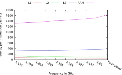
Figure 4.1 extracted from [35] shows a general overview of DRAM device structure. Each identified DRAM component consumes power. Based on [35] DRAM Array, power consumption scales accordingly to the memory bandwidth utilization. The larger the amount of accessed data, the higher the power consumption. The power consumption of I/O circuitry, is sensitive to both memory frequency and utilization. Indeed, as it is an interface between the DRAM array and the bus, it is also stressed when a large amount of data is requested. Finally, termination power, is adjusted to the bus electrical characteristics, and depends on its utilization. The sum of each power consumer defines the overall RAM dimm power consumption.
Basically, the overall RAM dimm power consumption scales with the bandwidth, since most of the components are bound to the bus utilization [35]. However, chang-ing the memory operatchang-ing frequency can reduce the overall power consumption. In electricity, based on Ohm’s law, P = U × I, where P is the power, U is the volt-age supply and I the current intensity. Lowering U means reducing P . As it is explained later in Chapter 6, the voltage is modified by changing the operating frequency. It is then interesting to modify the operating frequency to reduce the overall power consumption of the main memory. In addition, some RAM elements scale in U and others in U2 [93] when the frequency is changed. For the elements scaling in U2, significant power saving can then be obtained when lowering the op-erating frequency. Though reducing the RAM opop-erating frequency lowers the power consumption, it can impact the performances of an application that requests data into RAM. Consequently, lower performances, means increased application execu-tion time, increasing the system energy consumpexecu-tion. The whole game is then to reduce RAM operating frequency regarding bus utilization to reduce RAM energy consumption [35, 38, 108].
4.1.2 Possible Optimizations
DRAM exposes different operating frequencies. One can change the RAM dims operating frequencies, however the frequency shift has to be performed inside the
4.2. Disk 13 BIOS [35]. A machine reboot is then needed. For people looking for power savings on their laptops, no significant impact is observed on their working process. However in an HPC environment, rebooting a set of machine to achieve power reduction is not affordable. That is why most of existing optimization mechanisms [101, 35, 38, 108] rely on power models simulations and are not usable in the practical world. Nevertheless, Malladi et. al. [117] states that many datacenter applications stress memory capacity and latency but not memory bandwidth, therefore by replacing the high speed DDR3 with mobile DDR3, they demonstrate a 3-5 reduction factor on memory power with negligible penalties. However, the cost in infrastructure to operate such optimization is not affordable. Still, it enforce the need of being able to reduce the frequency at run-time. David et. al. [35] details the different steps and their complexity to allow RAM dynamic frequency scaling. As all manufacturers and HPC machine operators seek a maximum energy efficiency, it may happen in the future.
As explained in the introduction, RAM is not the only device that can be inter-esting to optimize because of its usage quantity. Disks also consume an important amount of power. Similarly to RAM dims they are permanently operated at their highest performance state, to prevent any performance loss. However, when a purely CPU bound application are run, disks never are on the critical path. They can be put into an idle state or even shut down to reduce the application power footprint.
4.2
Disk
As for RAM, scientific applications more and more rely on disks. The applications tackle ever bigger problems increasing their time to solution. The probability for a hardware failure during the computation can no longer be ignored. Then to prevent the application from losing all the performed computations in case of an hardware failure, check-pointing is performed [12]. In addition, a data protection mechanism is needed to protect the already stored data from any disk failures. Additional disks are then required. As shown in the small example above, for the TITAN machine 10000 disks are used if the considered size is 4TB. It can be more dramatic for data centers which are purely storage oriented. Being able to optimize the energy needed to write or read data or even shutdown unused disk can save a significant portion of the overall system energy consumption.
4.2.1 Power Consumers
Basically a non solid-state hard-drive is composed of multiple actors: spinning mag-netic platters, an arm moving the read/write head across the platters tracks and finally some electronic that hosts some buffers and the disk scheduler. Basically the power consumption can be divided into two parts. The power consumed in the mechanical parts and the power consumed in the electronic of control. When performing write or read operations the mechanical parts are the preponderant con-sumers. Then, the main idea to save energy is to prevent the mechanical parts to be permanently powered. In [77], the author shows that even at rest, i.e. not servicing requests, the mechanical parts still are the major consumer. Indeed, the magnetic platters always are rotating in order to grant the best response time then they are always consuming power. In [77], it is also shown that even when the magnetic platters are down the disk still consumes power. Indeed the electronic part is still
14 Chapter 4. Hard Drive and Memory Energy Consumption powered to acknowledge incoming requests in order to spin-up the magnetic platters back to their nominal speed. Multiple optimization scenarios can be derived from the different disk states and generally target the unnecessary power consumption generated by the mechanical part.
4.2.2 Possible Optimizations
Multiple optimization strategies [66, 134, 167] rely on the fact that in standby mode, all the mechanical components are shutdown. Once a disk is recognized as unused, it is put in standby mode. Though it cuts off almost the entire disk consumption, the cost to spin up the magnetic platters at its full speed is not negligible. It can be up to 4 times the average disk power consumption [77]. Moreover, as the rotation speed is a controlled system it takes some time to reach the nominal rotation speed. It has to be ensured that the disk will be powered long enough to counter that 4 times disk power pick. If not, the optimized disks will artificially consume more power. Others designed disks with dynamic speed control [61]. Instead of purely stopping the platters from spinning, different speed settings are used. The spin speed is then adapted to the request rate [108]. Some others would also consider data placement algorithms. As an example, putting the frequent data at a low Logical Block Number, i.e. the beginning of the disk, where more data can be fetched in one platter rotation [77]. Even though, it exists various ways to optimize Hard Drive energy consumption, all those optimizations are now embedded in current Hard Drives [40]. As for the previous section, it was also decided not to put additional efforts in designing power and energy optimization for Hard Drive Disks.
In the end, in the actual technology state the described optimization scenar-ios either are unusable in the practical world or are already embedded in current hardware. However, the increasing demand for checkpointing will increase the ap-plication dependency to disks. One way to leverage that is burst buffers [126, 163]. Data written by an application to a burst buffer is stored in a significant ram pool until they are stored on disks generally with a redundancy mechanism. The rising interests in burst buffers will further increase the demand for RAM dims or disks, certainly forcing manufacturers to provide more practical ways to optimize energy consumption.
However, for fans one practical way to modify their power consumption is by modulating their rotation speed. Though they are widely used to cool HPC com-puters or data centers, they are always used at their maximum speed. Therefore, the hardware is always kept at a cool temperature preventing failures due to over-heating. However, there is no need to use fans at their full speed since the hardware will operate the same way if the sustained temperature is 20◦C or 50◦C. Moreover, higher speeds mean higher power consumption. The next chapter presents a fan speed optimization technique to lower their energy consumption while preventing the processor to overheat.
Chapter 5
Fans
5.1
State Of The Art
Cooling systems are as important as the machine itself since they keep the hardware in a safe range of temperature and prevent failure due to overheating. Multiple ways to look at cooling systems exit. Two distinct approaches are generally considered to reduce cooling-related energy consumption in a data center or a supercomputer. The first is the general approach where the solutions make large-scale decisions. For instance, energy-centric job allocation [8, 13, 16] or task migration [53, 146, 147, 148] are typical systems helping to reduce energy dissipation. The second approach directly targets the air cooling and tries to reduce its consumption through precise tuning [76, 128]. The tool presented in this chapter, DFaCE considers a narrow scale: instead of considering the supercomputer as a whole, it considers nodes, enabling finer grain tuning.
At the server level, there are two different approaches of the cooling. Either by building theoretical models or by building dynamic systems to react according to what is observed on the system. The first category is about designing theoretical models to estimate the temperature induced by a given load or the best air cooling setting for a given temperature [67, 112, 138]. Rao et. al. [138] use such a theoretical model to determine the best CPU frequency according to the chip temperature. However, the model does not take into account the fan power consumption as DFaCE does. Moreover, even though DFaCE does not take into account processor frequency scaling to optimize the overall processor power consumption and not just its leakage, it can be transparently run concurrently to any Dynamic Voltage Frequency Scaling (DVFS) techniques to achieve the same purpose. Heo et. al. [67] and Liu et. al. [112] both propose models to quantify processor power leakage, however they are not used to control the fan speed.
At the opposite, other researchers propose using theoretical models with the goal of optimizing fan settings [155, 166]. Shin et. al. [155] theoretically model the effects of the temperature to simultaneously set the optimal fan speed and proces-sor frequency. Their system could lead to performance degradation since DVFS is considered as an option for cooling the CPU down. DFaCE only considers fans and therefore cannot degrade the programs performance. Similarly, Zhikui et. al. [166] propose a Fan Controller (FC) based on a theoretical model that sets the best fan speed for several fans as soon as the CPU load changes. FC, unlike DFaCE, does not consider power leakage: FC minimizes the fan power consumption while maintaining the system temperature at an arbitrary temperature threshold. The presented sys-tems consider theoretical analysis and models to determine an efficient fan setting. Therefore, the solutions suffer from bias induced by the approximations needed to model the complex temperature-related physics.
Theoretical models are built for a specific system or context and external events, such as fan failures or local hot-spots, cause them to be temporarily inaccurate as
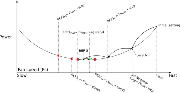
16 Chapter 5. Fans the models parameters may change without being reevaluated. DFaCE is not based on theoretical representations of the problem and does not have to approximate the problem because the effects of fan settings are directly evaluated on the computer it-self. Dynamic systems react according to what they observe on the system they run on; they do not suffer from the flaws of theoretical models. One such dynamic sys-tem, Thermal-Aware Power Optimization for servers (TAPO-server), was proposed by Wei et. al. [76]. TAPO-server regularly switches the fan speed to determine if the fan speed has to be increased or decreased in order to reach the minimal power consumption. The authors present convincing results, but TAPO-server does not take into consideration the quick variations of the heat generated by the device. It also restarts the learning process at every major system load change. Moreover, it is unable to handle more than one single fan; whereas, DFaCE is dedicated to mul-tiple fan control, allowing it to efficiently optimize the cooling power consumption. DFaCE also works in two distinct sequences: once the best setting is learned for a given load, it is immediately applied as soon as the load is observed again. Such knowledge capitalization and the ability to reuse the optimal learned fan settings is a key advantage over existing dynamic systems, which are currently unable to react as quickly as DFaCE.
Additionally, several mechanisms were described in the patent literature al-though they often are similar to the system presented before. For instance, many patents [41, 54, 91, 98] perform simple fan control close to what is achieved by thermal-directed fan control. The work described in [130, 58] is close to TACO-server and suffers from the same flaws.
5.2
Motivations
Although the CPU and the memory are often identified as the major consumers, the cooling system accounts for a non-negligible part of the overall energy consump-tion [57]. Except for some uncommon configuraconsump-tions [37, 29, 94], fans are still often in charge of cooling a computer. It is common for a PC to be cooled by several fans, each potentially consuming as much as 10W at full speed. As the fan power con-sumption can account for a large part of the total energy concon-sumption, depending on the number used, fans are a good target for energy optimization.
In general, the temperature of the main computer components impact the speed of the fans. A common for controlling system is thermal-directed [41, 54, 91, 98]: fans accelerate when the temperature increases in order to maintain the system tem-perature below an arbitrary threshold, which is often set to a conservative value. Thermal-directed fan control focuses only on temperature management, trying to avoid hardware failures due to overheating, and ignoring energy consumption. Typ-ically, it results in fans unnecessarily rotating at high speeds and consuming too much energy.
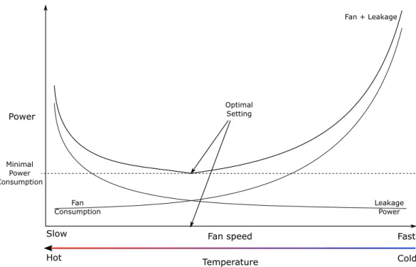
Moreover, slowing fans down increases the temperature and, apart from the increasing risk of hardware failures, it increases the power leakage of several compo-nents including the CPU. Leakage power is consumed due to transistor imperfection. Power leakage can represent up to 40% of current processor power consumption [112, 123]. Thus, efficiently managing fan speed consists in determining the opti-mal fan setting, which simultaneously minimizes the processor power leakage and fan power consumption, oversimplifying it would be "cooling enough but not too much". Figure 5.1 illustrates the impact of fan speed where the optimal fan setting
5.3. Power Characterization 17 Power Fan speed Temperature Slow Fast Cold Hot Leakage Power Fan Consumption Optimal Setting Fan + Leakage Minimal Power Consumption
Figure 5.1: Illustrating the balance between fan power consumption and power leakage.
is the one leading to minimal power consumption from both CPU power leakage and fan power consumption. The optimal fan controller has to be able to perform a subtle fan control: it must optimize the power consumption of a computer by using fan speeds that simultaneously minimize fan consumption and power leakage. The fan controller, in this chapter only takes into account fan speed. It does not aim to optimize the airflow either, since it will add a non negligent overhead to an already long converging technique.
Finally, to be able to determine the optimum fan setting as shown in Figure 5.2, it requires a precise knowledge of the fans consumption and of the controlled processor power leakage.
5.3
Power Characterization
5.3.1 Fan Power
The fan power consumption is exponential to its speed. It is common behavior for fans [76, 166] and is shown in Figure 5.2. Different techniques can be used to measure the fan power consumption at different speeds. A straight forward approach consists in plugging a power meter directly onto the fan while controlling its power supply to vary its speed. Such an approach avoids any potential noise as only the fan power is measured, but it requires the fan to be extracted from the computer and to be independently controlled, which often is troublesome.
The actual method employed is based on a power meter, plugged to the com-puter, which measures the overall system power consumption. As the power meter measures the consumption on the wall as opposed to using probes, the method is non-invasive and more easily achieved. While maintaining the node in an idle state, a dedicated software controls the fan speed while the power meter measures the
18 Chapter 5. Fans 0 0.5 1 1.5 2 2.5 3 3.5 4 200 400 600 800 1000 1200 1400 1600 1800 Watt Fan speed (RPM) Fan Power (W)
Figure 5.2: Power consumed by a standard 120mm CPU fan at different speeds.
node consumption for different fan speeds. The power consumption is not exact if the fan is not completely shut down at the minimal speed setting. However, the relative power consumptions at different speeds are correct enough to determine the setting for minimal power consumption. This gives the system a lightweight tech-nique to compare power consumptions. Accepting the minimal setting as being a non-optimal consumption, the fan consumption can be considered null at its lower setting. The fan’s consumption for every speed is computed by a simple difference between the present and the minimal speed. Let pwf an(f s) be the whole system power consumption for a fan speed f s. The fan power consumption when the fan runs at speed f s is then computed as pwf an(f s)−pwf an(0). The power consumption measured with the current method is not exact if the fan under evaluation is not completely shut down at the minimal speed setting. However, the relative power consumptions at different speeds are correct, which is sufficient to build a power profile of each fan speed. The higher the speed, the higher the power consumption. When considering Figure 5.2, high fan speeds must indeed be avoided. However, small speed variations at the highest fan speed provides significant power savings. Power consumption profiles depend on the fan model, so different fans may lead to different potential gains. The profile presented in Figure 5.2 is representative of the general case.
The fan used for Figure 5.2 is a large fan, similar to the ones usually found in desktop computers. However, fans used to cool down cluster nodes are, in general, smaller fans, operating at higher speeds, consuming more than 10W at full speed. In some cases, they even account for up to 20% of the total node power consump-tion [166]. As a result, greater power savings may then be expected when optimizing a cluster node compared to the desktop computer.
5.3. Power Characterization 19 By using the presented methodology, a power consumption profile is built for every connected fan. Such characterization is performed only once, to limit the on-line overhead. By using the power profiles, the optimization mechanism presented later will choose among the fan speeds the best one regarding the processor leak-age and fan power consumptions. However, to grant the system the possibility to also acknowledge the impact of different fan speeds on processor power leakage, an accurate leakage profile has to be built.
5.3.2 Power Leakage
As a reminder to find the optimal fan setting, the processor leakage is also needed. The power leakage is specific to CPU model since it mainly comes from imperfections within the fabric. The CPU leakage is consumed in three areas [129]. The leakage current is the current either going through the substrate or through a not fully closed transistor. The recharge current is due to parasitic capacitance of wires and inputs. Finally, the shoot-through current happens during the CMOS transistor commutation. Equation 5.1 summarizes the three leakage composing the leakage power.
Pleak = Pcurrent+ Pcapacitance+ Pcommutation Pcurrent = IL× U = U2 RL Pcapacitance= U2× CP × f Pcommutation = U2× f RS (5.1) With Pleak as the total leakage power, Pcurrent the loss due to leakage current, Pcapacitance the loss in parasitic wires capacitance, and finally Pcommutation lost tran-sistors commutation. U is the CPU supply voltage, IL and RL characterize the inductance and resistance of the substrate. CP is the wire capacitance, the longer the wire, the higher the capacitance is. RS represents the resistance of all the com-ponents on the path from the voltage supply and the ground. Finally, f is the CPU’s working frequency. Each one of them is squared proportionals to the supply voltage and/or linear proportional to CPU frequency. Moreover, the leakage power Pleak is also linear proportional to the die temperature [112]. As fan settings impact the processor temperature, by substitution it also impacts the CPU power leakage, then to correctly measure the power leakage the fan must be stopped. Moreover, as shown in Chapter 6, the processor have the ability to change on the fly its operating frequency and thus its voltage supply level. If the voltage varies, the power leakage will also vary as shown in Equation 5.1. Then by forcing the hardware to use only one frequency, the supply voltage remains constant, allowing to measure the leakage power evolution regarding the die temperature.
Algorithm 1 CPU intensive kernel used to generate CPU heat. num = srandom(42)
while true do res += sqrt(num) end while
20 Chapter 5. Fans To measure the leakage, the fans are stopped and a single frequency level is set. An artificial compute intensive task, presented in Algorithm 1, is then launched. The chosen load forces the CPU to increase its temperature. To ensure that a wide range of temperatures are reached, the multiple instances of the same benchmark are launched in parallel on the different processor cores.
A wide range of temperatures is obtained, from the ambient temperature when the processor is idle, to the critical temperature when the processor is heavily loaded as shown in Figure 5.3. To achieve such range of temperatures, the fans are also shut down to allow the CPU to heat up. Algorithm 2 shows the used methodology to achieve different CPU temperatures.
Algorithm 2 CPU heat generation and measurements CP U _F req = max
for Core=0 to maxNbCore do kill all kernel instance repeat
f ans_speed = max until system is cooled down
/* stop all the fans */ f ans_speed = 0
/* launch one instance per Core */ CPU-kernel(Core)
for sample=0 to 400 do
measure power and temperature sleep 1 second
end for end for
Firstly, the CPU is cooled down as much as possible to allow all the CPU cores to start at the same temperature. All the fans are then shut down to allow the processor to get beyond 60 degrees Celsius. After that, the stress is started while periodically measuring the power consumption and the temperature. When the current CPU load is fully sampled the next load level is started. At the end, a temperature and power consumption profile is available for each stress level. Figure 5.3 displays the available data. The y-axis displays each sample power consumption regarding the load level and the x-axis displays the range of reached temperatures. Each floor is obtained by increasing the number of concurrent benchmark execution. Due to the leakage power a slight increase on the power consumption can be observed for each load level while the temperature increases.
Due to the increased CPU activity a huge gap between each load level can be seen in figure 5.3. Generally, the consumed power is approximated as follows [27, 42, 50, 165, 162]:
P = Pdynamic+ Pstatic Pstatic ≃ cst
Pdynamic≃ A × C × V2× f (5.2)
As shown in Equation 5.2 the full CPU power consumption P is function of the power consumed while performing operations Pdynamic and of Pstatic. The leakage
5.3. Power Characterization 21 power presented in Equation 5.1 is considered constant for a fixed frequency and temperature. The gaps between the different processor loads are due to the increased Pdynamic. The dynamic power is a function of A the percentage of active gates, C the total capacitance load, V the supply voltage, and f the processor frequency. As the experiment is run on the same processor with a fixed frequency and voltage, C, V and f remains unchanged between two different load executions. However, as more cores are used, the percentage of active gates raises, increasing A. The activity factor is then solely responsible for the gaps between consecutive load executions.
It can also be noticed on Figure 5.3 that for some temperature ranges, such as [48-50], [57-59], and [63-73], two power consumptions are available. As explained above, the difference between them comes from an increased number of used gates and can be expressed as follows. P 2, and P 1 are the two power consumptions obtained for the same temperature and P 2 > P 1.
P 2 − P 1 = (PN Bcore+1+ Pleak)(PN Bcore+ Pleak) P 2 − P 1 = PN Bcore+1− PN Bcore P 2 − P 1 = C × ×V2× f × (A2− A1)
P 2 − P 1 ∝ A2− A1 (5.3)
As told above the power leak is considered as constant for a fixed temperature and frequency, Pleak can dropped from the equation. Only the dynamic powers PN Bcore+1 and PN Bcore remain. As the same processor, frequency and voltage are used for the two executions, the difference P 2 − P 1 is proportional to the difference of activity factors. 20 30 40 50 60 70 40 50 60 70 80 Watt Temperature (˚C)
1 thread 2 threads 3 threads 4 threads
Figure 5.3: Power consumption of a Intel Core i5 2380P processor at different tem-peratures.
22 Chapter 5. Fans For each point belonging to the same overlapping temperature range, the differ-ence between the two activity factors remain the same since the hardware has not changed. Then by subtracting the increased activity factor to all the points belong-ing to the same overlapped ranged, its impact on the measured power consumption is nullified. The leakage power then is the only factor responsible for power increase regarding temperature as shown in Figure 5.4.
Number of load’s thread Power difference (W) Standard deviation
One vs Two 9.98 4.82%
Two vs Three 10.52 4.62%
Three vs Four 11.92 4.26%
Table 5.1: Power cost of using an extra processor core
The difference between each consecutive thread load seems to be 10W when considering the overlapping temperature ranges on Figure 5.3. Table 5.1 shows the exact extra cost for each number of used cores. The column power difference shows the constant value subtracted to each point of consecutive higher load. For example, 9.98 W were subtracted to each power setting measured while using a two thread load. The column standard deviation shows the variation noticed for each overlapped point. As all standard deviations are lower than 5% the cost of using an extra core is considered as constant. The result of the normalization is displayed in Figure 5.4. 15 20 25 30 35 35 40 45 50 55 60 65 70 75 80 Watt Temperature (˚C)
1 Thread 2 Threads 3 Threads 4 Threads
Figure 5.4: Normalized Power consumption of a Intel Core i5 2380P processor at different temperatures.
In Figure 5.4 it can now be clearly see the power increase due to the temperature. Similar to the method employed to deduce fan power consumption, power leakage is calculated by a simple difference based on the data displayed in Figure 5.4. Let