HAL Id: halshs-00552993
https://halshs.archives-ouvertes.fr/halshs-00552993
Preprint submitted on 6 Jan 2011
HAL is a multi-disciplinary open access archive for the deposit and dissemination of sci-entific research documents, whether they are pub-lished or not. The documents may come from teaching and research institutions in France or abroad, or from public or private research centers.
L’archive ouverte pluridisciplinaire HAL, est destinée au dépôt et à la diffusion de documents scientifiques de niveau recherche, publiés ou non, émanant des établissements d’enseignement et de recherche français ou étrangers, des laboratoires publics ou privés.
Environment Quality Matter?
Alassane Drabo
To cite this version:
Alassane Drabo. Impact of Income Inequality on Health: Does Environment Quality Matter?. 2011. �halshs-00552993�
Document de travail de la série Etudes et Documents
E 2010.06
Impact of Income Inequality on Health:
Does Environment Quality Matter?
Alassane DRABO1
CERDI - University of Auvergne - France
Janvier 2010
1
Abstract :
This paper examines the link between health indicators, environmental variables and income inequalities. Theoretically, all the mechanisms developed in the literature underline a negative impact of income inequality on health status. However, empirical studies find different results and the conclusions are far from a consensus. In this paper we investigate how environment degradation could be considered as a channel through which income distribution affects population health. We first develop a simple theoretical model based on Magnani (2000), in which relative income affects health status through the level of pollution abatement expenditures. Our econometric analysis shows that income inequalities negatively affect environmental quality and environment degradation worsens population’s health. This negative effect of income inequalities on environment is mitigated by good institutions. We also show that income inequalities negatively affect health status. Another interesting result is that when environmental variables are taken into account, the level and the statistical significance of the coefficient of income inequality variable vanish. This confirms that environment quality is an important channel through which income inequalities affect population health. These results hold for air pollution indicators (CO2 and SO2) and water pollution indicator (BOD). It is also robust for rich and developing countries. Countries with high income inequalities may implement distributive policies in order to avoid its negative impact on health.
Keywords: health status, income inequality, environmental quality, instrumental variables method JL classification: C13, D63, I1; Q5
1. Introduction
Population health is an important economic concern for many developing countries. It plays a crucial role in development process, since it constitutes a component of investment in human capital and workforce is the most abundant production factor in these countries. It constitutes also a major preoccupation for the international community, especially when it is considered as a public good. The importance given to health status could be illustrated through its relatively high weight among the Millennium Development Goals (MDGs), of which three are related to health preoccupations. It is therefore important to know the factors that influence population health in order to undertake suitable economic policy.
Rodgers (1979) is one of the first economists to consider income distribution as a determinant of health outcomes. He shows that income inequality influences health status not only in developed countries, but also in developing countries, opening the debate about the association between income distribution and health. Wilkinson (1992) reopens the debate by showing through eleven industrialized countries that income inequality is an essential determinant of health status. Even though major part of the studies on this topic confirm the negative effect of inequality on health, some authors reject this hypothesis and show that high inequality may be indifferent to health status or improve it (Pampel et Pellai 1986 ; Mellor et Mylio, 2001; Deaton, 2003).
All the mechanisms through which income distribution impacts health status developed in the literature show that an increase in inequality worsens population health. These mechanisms rely on the absolute and relative income hypothesis, psychosocial hypothesis and neo-materialism hypothesis as well. In this paper we add the environment as another mechanism through which income distribution could affect health status. During the past fifteen years, with the emergence of environmental concerns, many studies examine the association between income inequality and natural environment quality. But they found different results. On the one hand, some show that more inequality may improve environment quality (Scruggs, 1998; Ravallion et al., 2000). On the other hand, other studies underline the negative impact of inequality on environmental quality (Boyce, 1994; Torras & Boyce, 1998). If environmental quality is degraded by an increase in inequality, it may be a channel that reinforces the negative effect of the other mechanisms. But if it is improved by an increase in inequality, it maybe a mechanism that mitigates or cancels the negative effect predicted by the other mechanisms and justify the discrepancies between the findings.
Our results show theoretically and empirically that an increase in income inequality is associated to environmental degradation and environment quality is an important determinant of health status. This negative effect of income inequality on environment quality is mitigated by good institutions. When the effect of environment quality on health is taken into account, the effect of income distribution on health decreases and become less significant statistically. That is, an increase in inequality worsens population’s health via environmental degradation. The rest of this paper is organized in four sections. Section 2 reviews the literature on the association between income distribution, environmental degradation and population’s health. In this section we explain why and how income inequality affects health before introducing the arguments that defend the association between income distribution and environmental quality. Section 3 develops a theoretical model in which income distribution affects health through environmental degradation. In section 4, we investigate empirically the effects of income distribution on health via environment quality. The last section concludes.
2. Literature review
The relationship between income inequality and population health has been investigated by many macroeconomic studies during the past 15 years. Scholars examine how and why income inequality affects health theoretically and empirically within and between nations. We will first review the traditional mechanisms, namely the ways income distribution affects population’s health already developed in the literature. Then, we will explain how income inequality impacts health through environmental degradation.
2.1. Traditional effects of income inequality on health
Theoretically, four mechanisms are underlined, through which income inequality can harm directly population health (Mayer & Sarin, 2005).
The first mechanism is the absolute income hypothesis. In fact, income may be an important determinant of population health, since it allows them to buy better nutrition or medical care or reduces their stress. If the relationship between an individual income level and its health status is linear, an extra unit of income will have the same effect on health regardless of whether it goes to the rich or to the poor. In this case taking a unit of income from the rich and giving it to the poor will lower health status among the rich and raise it among the poor by exactly equal amounts, leaving the global health unchanged. The reality is that standard economic models predict that the health gains from an extra unit of income should diminish as income rises (Preston, 1975; Laporte, 2002; Deaton, 2003; Backlund et al., 1996; Babones, 2008), in other words, health should be a concave function of income. That is, a transfer of a unit of income from the rich to the poor might improve aggregate population’s health status. The second mechanism developed in the literature is the relative income hypothesis. The effect of economic inequality is likely to depend to some extent on the geographic proximity of the rich to the poor (Mayer & Sarin, 2005). In fact, if people assess their income by comparing themselves to their neighbours, the income of others can affect their health. The chronic stress provoked by this comparison may lower resistance to some diseases and cause premature death. For Wilkinson (1997), if individuals evaluate their well-being by comparing themselves to others with more income than themselves, increases in economic inequality will engender low control, insecurity, and loss of self esteem.
The third way developed in the literature through which income inequality may worsen population health is psychosocial hypothesis. Inequality can impact health through social comparisons by reducing social capital, trust and efficacy (Kawachi & Kennedy, 1997; Marmot & Bobak, 2000). According to Wilkinson (1996), income inequality worsens health because a low ranking in the social hierarchy produces negative emotions such as shame and distrust that lead to worse health via neuro-endocrine mechanisms and stress-induced behaviors such as smoking, excessive drinking, taking dangerous drugs, and other risky activities (Mayer & Sarin, 2005). Lynch et al. (2001) found weak associations between a variety of measures of the psychosocial environment, (distrust, belonging to organizations, volunteering, and efficacy), and infant mortality, but they found that economic inequality is strongly related to infant deaths.
Neo-materialism hypothesis is the fourth mechanism through which income inequality may harm health status. According to some authors defending this idea, income inequality affects health mainly through its effect on the level and the distribution of material resources (Coburn, 2000 and Lynch, 2000). This argument suggests that bad health could be the consequence of an increase in income inequality that reduces state spending on medical care, goods and services for the poor.
If theoretically, all the arguments found in the literature indicate a negative impact of income inequality on health status, empirical findings are far from a consensus. Lynch et al. (2004) review 98 aggregate and multilevel studies to examine the associations between income inequality and health. They conclude that overall, there seems to be little support for the idea that income inequality is a major, generalizable determinant of population health differences within or between rich countries. Income inequality may, however, directly influence some health outcomes, such as homicide in some contexts. Mayer & Sarin (2005) review ten studies that use cross-sectional data to estimates the association between economic inequality and infant mortality. Eight (8) of these ten (10) use cross-national data and produce eleven (11) estimates. Nine (9) find that more unequal countries have higher infant mortality rates, and two (2) (Pampel & Pellai, 1986; Mellor& Milyo, 2001) find that more unequal countries have lower infant mortality rates than countries with less inequality. Wilkinson & Pickett (2006) compiled one hundred sixty eight (168) analyses in one hundred fifty five (155) papers reporting research findings on the association between income distribution and population health, and classified them according to how far their findings supported the hypothesis that greater income differences are associated with lower standards of population health. They find that for eighty seven (87) of these studies the coefficient of income inequality is always statistically significant with the correct sign. Forty four (44) present mixed results and thirty seven (37) no significant coefficient. They explain the divergence of empirical finding by the size of area, choice of control variables and don’t find any explanation for some international studies.
We argue here that in addition to the traditional mechanisms through which income inequality degrades population’s health, found in the literature, there exists at least another channel through which income inequality may affect health, namely environmental quality.
2.2. Income inequality and environment
A large body of research has reported strong associations between income inequality and environmental degradation: most theoretical arguments explain how income inequality may improve environmental quality.
First, income inequality can increase environment protection through individual preference toward environmental quality. In fact, for a given level of average income, greater inequality means not only higher incomes for the rich, but also lower incomes for the poor. Assuming that the income elasticity of demand for environmental quality is positive2, and taking a unit of income from the poor and giving it to the rich increases the demand for environmental quality of the rich, but at the same time it decreases the demand of the poor. The net effect on environmental quality depends on whether the demand-income relation is linear, concave or convex (Scruggs, 1998; Boyce, 2003). If this relation is linear, the transfer will not have any effect on environmental quality since an extra unit of income will have the same effect on environmental demand regardless of whether it goes to the rich or to the poor. If the environmental demand is linked to income by a convex (concave) relation, the transfer of income from the poor to the rich will increase (decrease) environmental demand.
It is more convincing to assume that the wealthiest prefer more environmental quality than the poor for many reasons. First, economic theories suggest that the rich prefer less environmental degradation than the poor. This may be due to the fact that environmental quality is a superior good and demand increases faster than income (Baumol and Oates, 1988). This is one of the explanations behind the environmental Kuznets Curve (EKC) hypothesis (Grossman & Krueger, 1995). As argued by Scruggs (1998), greater demand for environmental protection
2
among the wealthiest is also expected to result in a greater willingness and ability to pay for more environmental protection. In addition, wealth increases individuals’ concern for the future, maybe because they expect higher life expectancies than the poorest or because it increases their concern for their children in the future. Another reason to explain why rich prefer more environmental quality is that environmental protests are usually composed of middle and upper classes, not the poor (Dalton, 1994).
Income inequality can also reduce environmental degradation through the marginal propensity to emit (MPE) as argue by Ravallion et al. (2000). According to these authors, each individual has an implicit demand function for carbon emissions since the consumption of almost every good implies some emissions either directly via consumption or indirectly via its own production. They call marginal propensity to emit (MPE) the derivative of this implicit demand function with respect to income. If poor people have a higher (lower) MPE than rich ones, a redistribution policy that reduces inequalities will increase (decrease) carbon emissions. One can assume that the poorests have higher MPE than wealthiests, first because less emission goods need high technology and are thus generally expensive. Therefore, the poorest cannot afford it. In addition, poor tend to use energy less efficiently than the rich, which entails a higher MPE (Ravallion et al., 2000).
If these arguments predict an improvement of environment quality channelled by income inequality, it is also largely argued by some authors that inequality may degrade environment rather than improving it.
Boyce (1994) is the first author to examine how income inequalities affect environmental degradation. He supports the hypothesis that greater inequality may increase environmental degradation and this for two reasons. First, he argues that a greater inequality increases the rate of environmental time preference for both poor and rich. In fact, when inequality increases, the poor tend to overexploit natural capital, because they perceive it as the only resource they have and the only source of income that can help them secure their survival. In addition, economic inequality often provokes political instability and risks of revolts. This leads rich people to prefer a policy that consists in exploiting the environment and investing the returns abroad rather than investing in the protection of local natural resources. Therefore, for Boyce an increase in inequality induces both rich and poor to degrade more their own environment. The second argument put forward concerns the power of the rich. Boyce (1994) argues that in a society with greater inequality, rich people are likely to have large political power and can heavily influence decisions on environmentally damaging projects. Such decisions are based on the competition between those who benefit from the environmentally degrading action and those who bear the costs of it. Boyce (1994) argues that rich people are generally the winners, while poor people tend to be the losers of the investments that have an ecological impact. Therefore, economic inequality favours the implementation of environmentally damaging projects and investments since it “reinforces the power of the rich to impose environmental costs on the poor” (Ravallion et al., 2000, p.6). Scruggs (1998) has criticized the hypotheses supported by Boyce. He states that the influence via cost-benefit analysis is based on two wrong assumptions. First, according to Scruggs, “evidence indicates that better off members of society tend to have higher environmental concern than those with lower income” (Scruggs, 1998, p.260). Moreover Boyce (1994) assumes that a democratic social choice criterion leads to higher environmental protection than a non-democratic decision process (i.e. a power-weighted social decision rule), while evidence suggests that this is not necessarily true.
Another theoretical argument to explain why more inequality leads to more degradation is developed by Borghesi (2000). He argues that “much of the theoretical environmental literature has stressed the need of cooperative solutions to environmental problems. In an unequal society this is more difficult to achieve than in an equal society since there are
generally more conflicts among the political agents (government, trade unions, lobbies etc...) on many social issues. In this sense, greater inequality can contribute to increase environmental degradation” (Borghesi, 2000).
In addition to these arguments, some theoretical model supports the environmental degrading effect of income inequality. It is the case of Magnani (2000) who examines the impact of income distribution on public research and development expenditures for environmental protection. Through a model in which social decisions are determined by the preferences of the median voter, she hypothesizes that income inequality reduces pro-environmental public spending due to a “relative income effect,” and higher inequality shifts the preferences of those with below-average income in favour of greater consumption of private goods and lower expenditure on environmental public goods.
Marsiliani and Renström (2000) have also recently investigated how income distribution affects political decisions on environmental protection. Through an overlapping-generations model, they show that the higher the level of inequality in terms of median-mean distance, the lower the pollution tax set by a majority elected representative. Therefore, inequality induces redistribution policies that distort economic decisions and lower production. Inequality may be negatively correlated with environmental protection as it leads to less stringent environmental policies.
It is a priori difficult to predict the effect of income distribution on environment quality theoretically even though degrading effect seems in our viewpoint more convincing. Let us see empirical findings.
Many authors have empirically studied the relation between income distribution and environment quality and their conclusions are quite not consensual. In appendix 1, we report nine (9) important papers and thirty one (31) studies on the association between income distribution and environment quality. Among these studies, ten (10) conclude that inequality improves environment quality, nine (9) find the opposite conclusion and twelve (12) don’t find any significant association. Let explore some of them.
Scruggs (1998) performs two cross-country empirical analyses to assess the effect of income inequality on the environment through pooled models. In the first one, four different pollutants (sulphur dioxide, particulate matter, fecal coliform and dissolved oxygen) are used as dependant variable in a panel of 22 up to 29 countries. The second investigation examines the impact of several variables on a composite index of environmental quality in a panel of 17 OECD countries. This index is constructed by combining five pollution indicators.
In the first case, he finds conflicting results: greater inequality improves environmental quality for one environmental indicator (particulates), whereas the opposite holds for the other indicator (dissolved oxygen). For the other indicators (sulphur dioxide, fecal coliform), the coefficients are not statistically significant. In the second analysis, income inequality decreases environmental degradation.
Through a panel of 42 countries in the period 1975-92, Ravallion et al. (2000) first estimate CO2 emissions as a cubic function of average per capita income and of population and time trend. They estimate their equation with fixed effect model and simple pooled model using ordinary least squares. They conclude that higher inequality within countries reduces carbon emissions. However, the impact of income distribution on the environment decreases at higher average incomes.
Borghesi (2000) performs an empirical analysis similar to that of Ravallion et al. (2000). He uses CO2 per capita as environmental variable and Gini from Deninger and Squire as income inequality indicator with a panel of 37 countries from 1988-1995. In the pooled OLS model, an increase in inequality lowers CO2 emissions, whereas it does not have a significant impact on CO2 emissions according to the FE model.
Magnani (2000) assessed the impact of inequality on R&D expenditures for the environment taken “as proxy for the intensity of public engagement in environmental problems” through pooled ordinary least squares and random effects estimations. Using a panel of 19 OECD countries in the period 1980-1991, he finds that higher inequality reduces environmental care, however, the effect is statistically significant at 5% level in the pooled ordinary least squares model only.
Using the principal components analysis, Boyce et al. (1999) estimate statistically a measure of inter-state variations in power distribution based on voter participation, tax fairness, Medicaid accessibility, and educational attainment levels. They find that income inequality, per capita income, race, and ethnicity affect power distribution in the expected directions. Inequality in power distribution is associated with lower environmental policies, and these in turn are associated with higher environmental stress. Both environmental stress and power inequality are associated with adverse public health outcomes.
Torras and Boyce (1998) examine the effect of income distribution on a set of water and air pollution variables using the Global Environment Monitoring System (GEMS) data, Gini index, adult literacy rates and an aggregate of political rights and civil liberties.
With a OLS estimation, they obtain mixed results on the environmental impact of income inequality. The Gini coefficient is positive for some environmental indicators and negative for others.
It is also possible that more environmental degradation increases income inequality. In fact, environmental degradation in many ways affects the livelihood of the poor. The poorest are vulnerable to environmental degradation since they depend heavily on natural resources and have less alternative resource. They are also exposed to environment hazards and are less capable of coping to environmental risks (Dagusta and Mäler, 1994; World Bank, DFID, EC, UNDP, 2002). Furthermore, the rich are more capable of looking after themselves from environmental diseases than the poorest.3
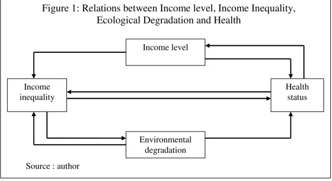
This review explains the complexity of the relation between income distribution and environment. Figure 1 summarizes the relation linking income inequality and population’s health.
3
This is not the object of the present study. Income inequality Health status Income level Environmental degradation
Figure 1: Relations between Income level, Income Inequality,
Ecological Degradation and Health
3. The model
The purpose of this model is to assess theoretically how income inequality affects health status through the level of pollution abatement expenditures. It consists in the introduction of health variable in Magnani’s model4. Let us assume an additively separable utility function for individual i:
( )
i i i i
U =c +
α
h Q (3.1)Where ci is the level of consumption of a private good and hi is the health status of individual i. We consider health not merely as absence of illness or infirmity, but also as a state of complete physical, mental and social well-being. hi is positively linked to
environment quality Q (a pure public good) and the effect of environment on health is the same for every individual i ( (∂hi) (∂Q)= ). k
α
i is the contribution of health to i’s utility. Itexpresses also the preference for environment quality as in Magnani’s model because if the contribution of health in individual i’s utility is high, he will prefer a better environment quality in order to improve his health. Furthermore, in this model, health is widely defined. The public good nature of Q implies that environmental policy E is necessary to solve market failure, that is Q=Q E( ), where E is public expenditures for environmental care, and
'(.) 0
Q > . Environmental care is financed through taxation by a fraction
τ
yi of individualincome yi and we have: E=Y(
τ τ
− 2 2), whereτ
is the environmental tax rate (τ∈(0,1)) and Y is the average income5.In this economy, individuals differ by personal income levels and income is distributed according to a unimodal function f y( )i where yi∈(0,yH) and yH is the maximum level of personal income. Income inequality implies that the majority of the population has income below the average and (ym Y) 1< , where ym is the median income of the distribution ( )f yi .
We assume that αi, the preference for environment quality and the contribution of health to utility is positively correlated with the individual relative income Ri =(y Yi ). This assumption is crucial for our analysis. That is, αi =αi(Ri) and
'
(.) 0
i
α > . The marginal rate of substitution between ci and hi depends on individual relative income. This assumption is
supported by some theoretical and empirical studies (Ng and Wang 1993, Konrad 1996 and Magnani 2000).
The indirect utility function for the individual i can be written as:
2
(1 ) ( 2)
i i i i
V = −τ y +αh Y τ τ− (3.2)
The optimal tax rate for individual i is obtained by differentiation of (3.2) with respect to
τ
and we have: τi*= −1 (1αik R) i. The marginal effect of relative income of individual i on his
ideal tax rate is: * ' 2
(∂τi) (∂Ri)= −( αi+αiRi) (kαi )= (1k
α
i)[
− + ∂1 (α
i ∂Ri)(Riα
i)]
. Thiseffect is positive ((∂τi*) (∂Ri)> ) if the relative income elasticity of the preference for 0
4
Magnani, E., Ecological Economics, 32 (2000) 431-443
5
The functional form for public environmental protection is quite general and expresses environmental cost of public funds (Magnani 2000).
environmental care εi is more than 1, or (∂αi ∂Ri)(Ri αi) 1> . For εi<1, the optimal tax rate
for individual i is a decreasing function of relative income.
If we are in a democracy with majority voting system, the politician will maximize the indirect utility function of the median voter according to the median voter theorem. The optimal tax rate chosen by the economy will be that of the median voter and we have:
*
1 (1 mk R) m
τ = − α (3.3)
Where m is the index for the median voter. This equation (3.3) shows that the equilibrium level of environmental abatement expenditure is function of income distribution.
* * * * 2
( , m ) ( ( ) 2)
E =E Y y Y =Y τ − τ (3.4)
And the marginal effect of income distribution on the optimal taxation rate is given by:
* ' 2 (∂τ ) (∂Rm)= −( αm+αmRm) (kαm)= (1k
α
m)[
− + ∂1 (α
m ∂Rm)(Rmα
m)]
(3.5) Where ' ( ) ( ) m m Rm α = ∂α ∂ is by assumption positive.The marginal effect of income inequality Rm on the optimal environmental public expenditure
* E is given by: * * * (∂E ) (∂Rm)=Y(∂τ ) (∂Rm) 1−τ (3.6) * (0,1)
τ ∈ , therefore 1−τ* > . The sign of 0 *
(∂E ) (∂Rm) only depends on the sign of
*
(∂τ ) (∂Rm). Environmental public expenditure is an increasing function of income equality
m
R if (1k
α
m)[
− + ∂1 (α
m ∂Rm)(Rmα
m)]
>0 and this condition holds if the relative income elasticity of the preference for environment care of the median voter is greater than one ( (∂αm ∂Rm)(Rm αm) 1> ).This result shows that income inequality affects negatively environmental public expenditure and therefore population’s health.
4. Empirical analysis
4.1. Estimations
The analysis is subdivided into three steps. We examine, first, the impact of income inequality on environmental quality. Then, we study the association between environment quality and health status. Finally, we compare the effect of income distribution on population’s heath in presence and in absence of environmental variables. The econometric relation between inequality and environment can be written as:
it i it k kit it
Where environment and EHII represent respectively the logarithm of environment quality and income inequality measure. Xk is the matrix of the control variables. The country fixed
effects are represented by λi and εit is the error term.
This equation could be estimated by the Ordinary Least Squares (OLS), but it is very likely that environmental degradation increases income inequality as explained in section 2. This potential simultaneity can be a source of endogeneity. Another source of endogeneity could arise from the measurement error of our inequality indicator. In order to solve this problem, we define as instrumental variable the dependency ratio and we estimate equation (4.1) with the Two Step Least Square (2SLS) method. As a proxy for demographic variable, age dependency ratio is an important determinant of income inequality because of its distributive effect and it is less convincing to ague that it affects directly environment quality. To control for the effect of income inequality depending on development level and institution quality, we progressively, add to equation (4.1), the interaction of income inequality with development level dummy and institution quality.
In the second model, health status is expressed as a function of environment quality and other explanatory variables.
it i it k kit it
Health =η +γenvironment +θ Z +ω (4.2) Where health represents health status measure and Zit is the matrix of the control variables.
i
η represents the country fixed effects and ωit is the error term. Equation (4.2) is estimated with standard fixed effects estimation.
The third model expresses health status as a function of income inequality with and without consideration of environmental variables. The coefficient of EHII must decrease with the addition of environmental variables if its effect is in part channelled by these variables.
it i it it k kit it
Health =φ ψ+ EHII +ρenvironment +σ Z +τ (4.3) This equation could be estimated by the Ordinary Least Squares (OLS), but it is very likely that population’s health affects income inequality through productivity, education and other factors. This potential simultaneity can be a source of endogeneity. To solve for this problem, we estimate equation (4.3) with the Generalized Method of Moments (GMM system).
4.2. Data and variables
The data used in this paper cover the period 1970-2000 subdivided into 6 periods of 5 years and we retain for the basic regression 90 developed and developing countries (because of data availability). As health variable we use the logit of under five survival rate (LOGIT SURVIVAL). The under-five survival indicator is limited asymptotically, and an increase in this indicator does not represent the same performance when its initial level is weak or high. The best functional form to examine that is where the variable is expressed into a logit form, as Grigoriou (2005) underlined. log survival= ln( ) 1 survival it survival − .
Data on under five mortality rates are from the World Health Organization (WHO).
The environmental quality is represented by three variables: the carbon dioxide emission per GDP (CO2), the biological oxygen demand (BOD) both taken from WDI 2007 and the sulphur dioxide emission per GDP (SO2) from Stern (2005). For these variables, a higher
value indicates more environmental degradation. CO2 and SO2 are air pollution indicators and BOD in a water quality indicator.
Income inequality is measured by the Gini coefficient taken from the database created by Galbraith and associates and known as the University of Texas Inequality Project (UTIP) database. It contains two different types of data on inequality: the UTIP-UNIDO and the EHII indexes. The EHII (that we use here) is an index (ranging from 0, low inequality to 1, high inequality) of Estimated Household Income Inequality and is built combining the information in the Deninger and Squire (D&S) data with the information in the UTIP-UNIDO data. The other variables used are gross domestic product per capita (GDPCAP), population density (POPDENS), fertilizer use (FERTILIZER), foreign direct investment (FDI), dependency ratio (DEPENDENCY) and trade openness (OPEN), all taken from WDI 2007 and primary school enrolment (SCHOOL) from Barro and Lee (2000).
Appendix 2 summarizes the characteristics of the important variables. This table shows the mean, the minimum, the maximum, the standard deviation and the coefficient of variation of each variable. These statistics are completed by appendix 3 which presents the correlation between important variables. These statistics are confirmed by appendix 7, which displays the statistical relation between EHII and environmental variables. These relations are just a simple correlation and don’t take into account the influence of other variables. The econometrical section will solve for this.
4.3. Results
4.3.1. Income inequality and environment
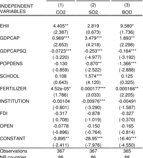
The results obtained from equation (4.1) for the whole sample of developed and developing countries (the relation between inequality and environment quality), are reported in table 1. The column 1 of this table shows the results when the logarithm of carbon dioxide emission per GDP (CO2) is used as environmental variable. The environmental Kuznets Curve (EKC) hypothesis is verified, since the coefficient of the logarithm of GDP per capita (GDPCAP) is positive and statistically significant, and the coefficient of its square (GDPCAPSQ) is negative and also significant. In this column, the coefficient of inequality variable (EHII) is positive and statistically significant at 5%, showing that an increase in income inequality worsens environmental quality.
Columns 2 and 3 summarize the results when sulphur dioxide emission per GDP (SO2) and the biological demand (BOD) are respectively used as environmental variables. The important results remain unchanged, namely, income inequality is an important cause of environment degradation, except for SO2 where the coefficient of inequality is not statistically significant. We estimated again equation (1) by adding as additional variable, the interaction between income inequality and economic development level dummy to assess the differential effect of income inequality depending on development level. The results obtained are summarized in the first three columns (1, 2 and 3) of appendix 4. The relationship between income inequality and environment is confirmed for CO2 in the first column. In this column, the coefficient of the interaction term is negative and statistically significant. This result shows that income inequality increases CO2 emission but the effect is higher in developed countries. For SO2 emission in column (2), only the coefficient of the interaction term is statistically significant and positive showing that income inequality increases SO2 emission only in developing countries. Finally for BOD in column (3), we have not any effect.
To take into account the role played by institutions quality on the inequality effect, we add as additional variable, the interaction between institution and inequality. The results are presented in the last three columns (4, 5 and 6) of appendix 4. These results show that good
institutions mitigate the negative effect of income inequality on environment quality, but this effect is only significant statistically for SO2 emission in column (5).
Table 1: Impact of income inequality on environment quality: 2SLS FIXED EFFECTS ESTIMATIONS
DEPENDENT VARIABLES
(1) (2) (3)
INDEPENDENT
VARIABLES CO2 SO2 BOD
EHII 4.405** 2.819 9.580* (2.387) (0.673) (1.736) GDPCAP 0.969*** 3.479*** 1.893** (2.653) (4.218) (2.298) GDPCAPSQ -0.0723*** -0.253*** -0.164*** (-3.220) (-4.977) (-3.192) POPDENS -0.130 -0.870** -1.366*** (-0.859) (-2.522) (-2.888) SCHOOL 0.108 1.574*** 0.125 (0.643) (4.120) (0.325) FERTILIZER 4.52e-05* 0.000177*** 0.000166** (1.786) (3.033) (2.205) INSTITUTION -0.00104 -0.00976*** -0.00491 (-0.801) (-3.290) (-1.587) FDI -0.317 -0.878 -0.327 (-0.708) (-1.019) (-0.370) OPEN -0.0778 -0.150 -0.165 (-0.896) (-0.764) (-0.814) CONSTANT -3.895** -28.95*** -16.40*** (-2.411) (-7.976) (-4.550) Observations 367 367 365 NB countries 86 86 88
***significant at 1%, **significant at 5%, *significant at 10%. t-statistics enter parenthesis. Income inequality (EHII) is instrumented by dependency ratio. The first step estimation results are presented in appendix 5.
4.3.2. Environment and health
The effect of environmental quality on health status (equation 4.2) is estimated with standard fixed effects model and the results are reported in table 2. Column 1 presents the results when environment quality is measured by CO2 emission. All the explanatory variables have expected sign and are statistically significant, except the primary school enrollment lagged (SCHOOL(1)) which is not statistically significant. GDP per capita lagged (GDPCAP(1)) and immunization rate (IMDPT) improve the survival rate while fertility rate (FERT) and environment quality (BOD) degrades it. The negative and significant coefficient of CO2 shows that air pollution worsens health status as expected in the literature review. Columns 2 and 3 shows the results when SO2 and BOD are respectively used as environmental indicators. All these columns underline the negative effect of air and water pollution on population’s health.
Table 2: Impact of environment quality on health OLS FIXED EFFETS ESTIMATION
Dependent variable: logit of under five survival rate INDEPENDENT VARIABLE (1) (2) (3) GDPCAP(-1) 0.396*** 0.290*** 0.282*** (6.223) (3.640) (3.883) IMDPT 0.502*** 0.474*** 0.532*** (5.710) (5.195) (5.632) SCHOOL(-1) -0.310 -0.206 -0.441 (-1.206) (-0.779) (-1.532) FERT -0.202*** -0.178*** -0.153*** (-5.933) (-4.835) (-4.343) CO2 -0.223* (-1.949) SO2 -0.209*** (-8.060) BOD -0.237*** (-4.711) CONSTANT 0.340 -3.056*** -2.073*** (0.582) (-4.711) (-3.088) Observations 434 429 373 NB countries 97 96 93
***significant at 1%, **significant at 5%, *significant at 10%. t-statistics enter parenthesis.
4.3.3. Income inequality, environment and health
The effects of income inequality on health status with and without consideration of environment variables (equation 4.3) are summarized in table 3. Column (1) of this table presents the results without consideration of environment quality. Each variable has the expected sign. Income inequality affects negatively and significantly population health. In the other columns (2, 3 and 4) of this table, we introduce environment quality in the model. All the environmental variables affect negatively health status. In addition, the introduction of environmental variables decreases the level and the statistical significance of the coefficient of income inequality variable in each column. This confirms the channel role played by environmental quality concerning the effect of income distribution on population health.
Table 3: Impact of income inequality and environment quality on health GMM System estimation results
Dependent variable: logit of under five survival rate Independent variables (1) (2) (3) (4) GDPCAP 0.799*** 0.774*** 0.766*** 0.495** (11.98) (11.14) (11.68) (2.455) IMDPT 0.547*** 0.550*** 0.585*** 0.500*** (4.678) (4.646) (5.112) (4.090) SCHOOL 0.180 0.482 0.230 0.264 (0.650) (1.579) (0.856) (1.469) FERT -0.125*** -0.147*** -0.119*** -0.226*** (-3.535) (-4.147) (-3.591) (-3.527) EHII -1.400** -1.200* -1.302** -1.103 (-2.144) (-1.709) (-2.067) (-1.133) CO2 -0.217** (-2.050) SO2 -0.0498** (-2.175) BOD -0.224* (-1.746) CONSTANT -3.109*** -2.916*** -3.901*** -3.243*** (-3.600) (-3.248) (-4.675) (-2.614) Observations 360 359 357 354 NB countries 90 89 88 90
Sargan OID test (p.value) 0.12 0.34 0.10 0.25
AR(2) 0.58 0.63 0.69 0.56
***significant at 1%, **significant at 5%, *significant at 10%. t-statistics enter parenthesis.
5. Conclusion
The purpose of this paper was to investigate the effect of income distribution on health which passes through environmental quality. Theoretically, we show that environment degradation could be consider as a channel through which income inequality affects population health in addition to the direct mechanisms found in the literature. This effect could reinforce the negative effect of income inequality on health.
Empirically, we show through an econometric analysis that income inequality affects negatively environmental quality and environment degradation worsens population’s health. This negative effect of income inequality on environment quality is mitigated by good institutions. Another interesting result is that income inequality affects negatively health status and in presence of environmental variable, the level and the statistical significance of the coefficient of income inequality variable decrease. This confirms that environment quality is an important channel through which income inequality affects population health. These results hold for air pollution indicators (CO2 and SO2) and water pollution indicator (BOD). It is also robust for rich and developing countries.
As policy implication, our results mean that income inequality is bad for health and environment, and countries with high income inequality may implement distributive policy in order to avoid its negative impact on health.
Next studies could extend our finding is taking it again at individual level (microeconomics). Another way to extend this article is to verify it conclusions for other environmental and inequality variables.
Bibliography:
Anand, S. & Ravallion, M., 1993. Human Development in Poor Countries: On the Role of Private Incomes and Public Services, Journal of Economic Perspectives 7, 133-50. Babones, S.J., 2008, Income inequality and population health: Correlation and causality,
Social Science & Medicine 66, 1614e1626
Backlund, E., Sorlie P. and Johnson N., 1996. The shape of the relationship between income and mortality in the United States: evidence from the national longitudinal mortality survey. Annals of Epidemiology, 6 pp.12-20
Baumol, W. & Oates, W., 1988. The Theory of Environmental Policy. Cambridge University Press, Cambridge, UK.
Bobak, M., Pikhart, H., Rose, R., Hertzman, C., and Marmot, M. (2000). Socioeconomic factors, material inequalities, and perceived control in self-rated health: cross-sectional data from seven post-communist countries. Social Science & Medicine, 51, 1343-1350.
Borghesi, S., 2000, Income Inequality and the Environmental Kuznets Curve, NOTA DI LAVORO 83.2000
Boyce, J. K., Andrew R., Klemer, Paul H., Templet, and Cleve E. W., 1999, Power Distribution, the Environment, and Public Health: A State-level Analysis, Ecological Economics 29: 127-140.
Boyce, J.K. 2003, Inequality and Environmental Protection, Political Economy Research Institute Working Paper, n° 52.
Boyce, R., 1994. Inequality as a cause of environmental degradation, Ecological Economics 11, 169–178.
Clément, M. & Meunie, A., 2008, Economic Growth, inequality and environment quality: An empirical analysis applied to developing and transition countries, Cahiers du GREThA n° 2008-13
Coburn, D., 2000, Income inequality, social cohesion and the health status of populations: the role of neo-liberalism, Social Science and Medecine, 51 pp.135-146
Dasgupta, P., & Maler, K, 1994. Poverty, institutions, and the environmental-resource base. Washington, D.C.: World Bank.
Dalton, R.,1994. The Green Rainbow: Environmental Groups in Western Europe. Yale University Press, New Haven, CT.
Deaton, A., 2003. Health, inequality, and economic development, Journal of Economic Literature, 41 pp. 113-158
Glazer, A. and Konrad, K.A., 1996. A signalling explanation for charity. Am. Econ. Rev. 86, 1019–1029.
Grigoriou, C., 2005, Essais sur la vulnérabilité des enfants dans les pays en développement: l’impact de la politique économique, Thèse pour le doctorat ès sciences économiques, Université d’Auvergne, Centre d’Etudes et de Recherches sur le Développement International
Grossman, G. et Krueger A.B., 1995, Pollution Growth and the environment, Quaterly Journal of Economics, 110, 353-377
Herring, N., Mulatu A. and, Bulte E., 2001, Income inequality and the environment: aggregation bias in environmental Kuznets curves, Ecological Economics 38, 359–367
Kawachi, I. & Kennedy B. P. 1997, Social Capital, income inequality, and mortality, American Journal of Public Health, 87(9), pp. 1491-1498
Knowles, S. & Owen P.D., 1994, Health Capital and Cross-country variation in income per capita in the Mankiw-Romer-Weil model, Economics Letter, vol. 48(1), 99-106
Laporte, A. 2002. A note on the use of a single inequality index in testing the effect of income distribution on mortality, Social Science and Medecine, 55 pp. 1561-1570
Lynch, H. W., Smith, G, Kaplan G. and House J. S. 2000. Income inequality and mortality: Importance to health of individual income, psychosocial environment and material condition, British Medical Journal, 320, pp. 1200-4.
Lynch, H. W., Smith, G. D., Hillemeier, M., Shaw, M., Raghunathan, T., and Kaplan, G., A. 2001. “Income Inequality, the psychosocial environment, and health: comparison of wealthy nations”. The Lancet, 358, 194-200.
Lynch, J., Smith, G. D., Harper, S., Hillemeier, M., Ross, N., and Kaplan, G. A., 2004, Is income inequality a determinant of population health? Part 1. A systematic review. Milbank Quarterly, 82, 5-99.
Magnani, E., 2000, The environmental Kuznets curve, environmental protection policy and income distribution, Ecological Economics, vol.32, pp.431-443.
Marsiliani, L. & Renström T.I., 2000, Inequality, environmental protection and growth, CentER working paper n.2000-34, Tilburg University, The Netherlands.
Marsiliani, L. & Renström T.I., 2000, Inequality, environmental protection and growth, CentER working paper n.2000-34, Tilburg University, The Netherlands.
Mayer, S. E. & Sarin A., 2005. Some mechanisms linking economic inequality and infant mortality. Social Science and Medecine, 60, pp.439-455.
Mellor, J & Milyo J., 2001, Reexamining the evidence of an ecological association between income inequality and health. Journal of Health Politics, Policy and Law, 26, (3), pp. 487-522.
Ng, Y.-K. and Wang, J., 1993. Relative income, aspiration, environmental quality, individual and political myopia. Math. Social Sci. 26, 3–23.
Pampel, F. & Pellai, V., 1986, Patterns and determinants of infant mortality in develeloped nations, Demography, 23(4), pp. 525-541.
Preston, S. H., 1975, The Changing Relation Between Mortality and Level of Economic Development, Population Studies, 29(2), 231-248.
Ravallion, M., Heil M. and Jalan J., 2000, Carbon emissions and income inequality, Oxford Economic Papers, 52:651-669
Rodgers, G. B., 1979, Income and Inequality as determinants of mortality: An international cross-section analysis. Population studies, 32 pp.343-351
Scruggs, Lyle A., (1998), Political and economic inequality and the environment, Ecological
Economics, 26, 259-275
Torras, M. & Boyce, J.K., 1998. Income, inequality, and environmental quality: An international cross-sectional analysis. Ecological Economics 25, 147–160.
Wilkinson, R. G. 1996, Unhealthy Societies: the Afflictions of Inequality, London, England: Routledge.
Wilkinson, R. G., 1997. Income inequality and social cohesion, American Journal of Public Health, (87) pp. 104-106
Wilkinson, R. G., & Pickett, K. E., 2006. Income inequality and population health: a review and explanation of the evidence. Social Science & Medicine, 62, 1768-1784.
Wilkinson, R.G., 1992, Income Distribution and Life Expectancy, British Medical Journal, 304, p. 165-168
World Bank, Department for International Development (DFID) UK , European Commission (EC) & United Nations Development Program (UNDP), 2002, Linking Poverty
Appendices:
Appendix 1: literature review
effect of inequality study year inequality
variable
environment measure
effect Level sig.
data estimator review other covariates
SO2 emission impr. 10% Clément
and Meunie 2008 gini
WIDER BOD emission degr. 1%
83 developing and transition countries in 1988-2003 OLS Cahiers du GRETh A n° 2008-13 GDP, GDP², GDP 3 access to safe water, access to sanitation, and deforestation degr. 1% carbon dioxide emissions, nitrogen depletion, and phosphorus depletion impr. 1% Herring, N., Mulatu A. and, Bulte E. 2001 gini index sulfur dioxide and particulate concentrations impr. NO 16-country sample of sub-Saharan African countries pooled Ecologi cal Econo mics 38, 359– 367 GDP, GDP² impr. 1% OLS pooled model Borghesi 2000 Gini (Deninge r and Squire)
CO2 per capita
degr. NO panel of 37 countries from 1988-1995 fixed effects NOTA DI LAVOR O 83.2000 GDP, GDP², GDP3, Population density, industry share. simple OLS degr. ML Marsiliani and Renström 2000 ratio of househol ds ranked at top 90th percentile to the median househol d sulfur, Nitrogen oxides and carbon dioxide impr. 1% two panels of 7 and 10 industriali zed countries over 1978-1997 fixed effects CentER workin g paper n.2000-34 GDP quintiles 1 / quintiles 4 10% Magnani 2000 gini Public R&D expenditure for environmental protection degr. NO 17 developed countries fixed effects & random effects Ecologic al Economi cs 32 (2000) 440 431–443 GDP, GDP², Time trend
effect of inequality study year inequality
variable
environment measure
effect sig. Level
data estimator review other covariates
Ravallion M., Heil M., Jalan
2000 gini index CO2 per capita
emission impr. 5% panel of 42 countries in the period 1975-92 fixed effects & pooled OLS Oxford Econo mic Papers, 52 :651-669 GDP, GDP², Population
Boyce et al. 1999 power inequality environment policy degr. 1% 50 US states in 1990's OLS Ecologic al Economi cs 29 (1999) 127–140 manufacturin g share, urbanization and population density sulfur dioxide impr. 1%
particulate
matter impr. NO fecal coliform degr. NO Scruggs L.A. 1998 Gini (Deninge r and Squire) dissolved oxygen degr. 1% 25–29 countries for 3 periods: 1979– 1982, 1983–1986 and 1987– 1990 OLS pooled model Ecologic al Economi cs 26 (1998) 259–275 Democracy, Income, Industrialize site, periode
Sulfur dioxide degr. 1% Smoke degr. 1% Heavy particles impr. 1%
Dissolved
oxygen impr. 1% Fecal coliform impr. NO Safe water (%) degr. 1% gini (low
income)
Sanitation (%) degr. NO Sulfur dioxide impr. 1% Smoke impr. NO Heavy particles degr. NO
Dissolved
oxygen degr. NO Fecal coliform impr. 1% Safe water (%) degr. NO Torras and Boyce 1998 gini (high income) Sanitation (%) degr. NO 287 stations in 58 countries OLS Ecologic al Economi cs 25 (1998) 147–160 GDP, GDP², GDP3, literacy rate, right
Appendix 2: descriptive statistics
MEAN MINIMUM MAXIMUM COEF. VAR. STAND. DEV. NB. OBS. LOGIT SURVIVAL 2.988 0.672 5.293 0.406 1.214 478 CO2 0.448 0.020 2.255 0.747 0.335 436 BOD 2.34e-06 2.29e-07 0.00002 1.034 2.42e-06 369 SO2 8.18e-09 5.64e-12 2.99e-07 3.320 2.72e-08 485 EHII 0.417 0.266 0.642 0.147 0.061 485 GDPCAP 6280 122.6 36160 1.261 7922 485 SCHOOL 0.304 0 0.93 0.889 0.271 485 IMDPT 0.710 0.012 0.99 0.350 0.249 351 FERT 3.997 1.18 8.494 0.492 1.968 485 POPDENS 98.713 1.567 951.97 1.265 124.89 485 FERTILIZER 1681.06 0.896 37358 2.201 3700.6 485
Appendix 3: correlations between important variables
LOGIT
SURVIVAL CO2 BOD SO2 EHII GDPCAP SCHOOL IMDPT FERT POPDENS
LOGIT SURVIVAL 0.94* LIFE EXPECT 0.30* 1.00 CO2 -0.45* 0.01 1.00 BOD -0.19* 0.06 0.20* 1.00 SO2 -0.62* -0.17* 0.13* 0.11* 1.00 EHII 0.81* 0.17* -0.47* -0.14* -0.61* 1.00 GDPCAP -0.86* -0.29* 0.33* 0.12* 0.52* -0.63* 1.00 SCHOOL 0.64* 0.17* -0.20* -0.03* -0.30* 0.44* -0.59* 1.00 FERT -0.90* -0.30* 0.32* 0.22* 0.57* -0.68* 0.84* -0.61* 1.00 POPDENS 0.17* -0.01 0.12* -0.11* -0.11* 0.11* -0.12* 0.05 -0.25* 1.00 FERTILIZER 0.40* 0.02 -0.11* -0.08* -0.27* 0.41* -0.31* 0.25* -0.32* 0.12* *significant at 10%.
Appendix 4: Development level and institution conditional impact of inequality on environment
DEPENDENT VARIABLES (2SLS FIXED EFFECTS ESTIMATIONS) DEVELOPMENT LEVEL INSTITUTION QUALITY
(1) (2) (3) (4) (5) (6)
INDEPENDENT
VARIABLES CO2 SO2 BOD CO2 SO2 BOD
EHII 12.14*** -7.513 5.685 6.481** 15.10 14.17* (3.576) (-0.892) (0.652) (2.410) (1.405) (1.955) (EHII)x(DEV_LEVEL) -9.984*** 13.31* 5.757 (-3.149) (1.698) (0.723) (EHII)x(INSTITUTION) -0.129 -0.778* -0.247 (-1.290) (-1.929) (-1.169) GDPCAP 1.606*** 2.623** 1.523 0.930** 3.276** 1.775** (3.649) (2.412) (1.427) (2.344) (2.059) (2.097) GDPCAPSQ -0.118*** -0.192*** -0.138** -0.0686*** -0.230** -0.154*** (-4.178) (-2.734) (-1.993) (-2.807) (-2.343) (-2.909) POPDENS -0.0352 -0.995*** -1.477*** -0.162 -1.016 -1.484*** (-0.240) (-2.735) (-2.931) (-0.963) (-1.500) (-2.927) SCHOOL 0.161 1.506*** 0.0934 0.285 2.570*** 0.442 (0.958) (3.616) (0.225) (1.239) (2.832) (0.916) FERTILIZER 5.00e-05** 0.000171*** 0.000173** 6.27e-05** 0.000254** 0.000199**
(1.971) (2.689) (2.168) (1.996) (2.087) (2.350) INSTITUTION -0.00313** -0.00700* -0.00386 0.0556 0.334* 0.104 (-2.097) (-1.890) (-1.036) (1.267) (1.875) (1.118) FDI -0.295 -0.846 -0.350 -0.0841 -0.995 -0.407 (-0.666) (-0.908) (-0.369) (-0.164) (-0.597) (-0.446) OPEN -0.0770 -0.154 -0.175 -0.133 -0.376 -0.242 (-0.895) (-0.724) (-0.804) (-1.275) (-0.940) (-1.098) CONSTANT -6.442*** -25.52*** -14.92*** -4.806** -34.81*** -18.03*** (-3.367) (-5.415) (-3.241) (-2.481) (-4.449) (-4.447) Observations 367 367 365 367 367 365 NB countries 86 86 88 86 86 88
***significant at 1%, **significant at 5%, *significant at 10%. t-statistics enter parenthesis. Income inequality (EHII) is instrumented by dependency ratio; (EHII)x(DEV_LEVEL) is instrumented by the interaction between dependency ratio and
development level dummy and EHII INSTITUTION is instrumented by the interaction between dependency ratio and institution variable. The first step estimation results are presented in appendix 5.
Appendix 5: First step estimation results
DEPENDENT VARIABLES (FIRST STEP ESTIMATIONS)
(1) (2) (3)
INDEPENDENT VARIABLES EHII (EHII)x(DEV_LEVEL) (EHII)x(INSTITUTION)
GDPCAP -0.146*** -0.096* -1.644 (-2.99) (-1.93) (-0.94) GDPCAPSQ 0.0079*** 0.0048 0.085 (2.63) (1.53) (0.77) POPDENS 0.047*** 0.035*** 0.531 (3.46) (2.63) (1.13) SCHOOL 0.0023 0.015 1.528 (0.08) (0.56) (1.56)
FERTILIZER -8.14e-06** -6.06e-06* -0.000022
(-2.48) (-1.93) (-0.20) INSTITUTION 0.0003 0.000058 0.521*** (1.54) (0.29) (13.73) FDI 0.063 0.044 2.284 (0.88) (0.64) (0.91) OPEN 0.0036 -0.0026 -0.332 (0.25) (-0.19) (-0.67) DEPENDENCY -0.003*** 0.00024 -0.020 (-3.24) (0.18) (-0.54) (DEPENDENCY)x(DEV_LEVEL) -0.0042*** (-2.66) (DEPENDENCY)x(INSTITUTION) -0.0018** (-2.04) Observations 367 367 367 NB countries 86 86 86
Appendix 6: data characteristics and sources
VARIABLES CHARACTERISTICS SOURCES
LOGIT SURVIVAL
logit of survival rate (log
survival/log(1-survival)) WHO
LIFE EXPECT modified life expectancy (-log(80-life
expectancy)) WDI 2007
CO2 carbon dioxide emission as ratio of
GDP WDI 2007
BOD biological oxygen demand as ratio of
GDP WDI 2007
SO2 sulfur dioxide emission as ratio of
GDP Stern 2004
EHII Estimated Household Income Inequality
University of Texas Inequality Project (UTIP) database
DEPENDENCY Population under 15 and above 65 WDI 2007 INSTITUTION Political institution quality Polity IV GDPCAP Gross Domestic Product per capita WDI 2007
SCHOOL Primary school enrollment WDI 2007
IMDPT Immunization rate WDI 2007
FERT fertility rate WDI 2007
POPDENS population density WDI 2007
FERTILIZER fertiliser use WDI 2007
Appendix 7: Correlation between income inequality and environment quality
-3 0 -2 5 -2 0 -1 5 lo g (s o 2 ) .2 .3 .4 .5 .6
income inequality (ehii) Fitted values log(so2) Correlation between log(so2) and inequality
-1 8 -1 6 -1 4 -1 2 -1 0 lo g (b o d ) .2 .3 .4 .5 .6
income inequality (ehii) Fitted values log(bod) Correlation between log(bod) and inequality
Appendix 8: Country list
World bank code country World bank code country
ARG Argentina JOR Jordan
AUS Australia JPN Japan
AUT Austria KEN Kenya
BDI Burundi KOR Korea, Rep.
BEL Belgium KWT Kuwait
BEN Benin LBR Liberia
BGD Bangladesh LKA Sri Lanka
BOL Bolivia LSO Lesotho
BRA Brazil MEX Mexico
BWA Botswana MOZ Mozambique
CAF Central African Republic MUS Mauritius
CAN Canada MWI Malawi
CHL Chile MYS Malaysia
CHN China NIC Nicaragua
CMR Cameroon NLD Netherlands
COG Congo, Rep. NOR Norway
COL Colombia NPL Nepal
CRI Costa Rica NZL New Zealand
CYP Cyprus PAK Pakistan
DEU Germany PAN Panama
DNK Denmark PER Peru
DOM Dominican Republic PHL Philippines
DZA Algeria PNG Papua New Guinea
ECU Ecuador POL Poland
EGY Egypt, Arab Rep. PRT Portugal
ESP Spain PRY Paraguay
FIN Finland RWA Rwanda
FJI Fiji SEN Senegal
FRA France SLE Sierra Leone
GBR United Kingdom SLV El Salvador
GHA Ghana SWE Sweden
GMB Gambia, The SWZ Swaziland
GRC Greece SYR Syrian Arab Republic
GTM Guatemala TGO Togo
HND Honduras THA Thailand
HTI Haiti TTO Trinidad and Tobago
HUN Hungary TUN Tunisia
IDN Indonesia TUR Turkey
IND India UGA Uganda
IRL Ireland URY Uruguay
IRN Iran, Islamic Rep. USA United States
ISL Iceland VEN Venezuela, RB
ISR Israel ZAF South Africa
ITA Italy ZMB Zambia