Design method for centrifugal compressor and centripetal turbine impellers

DESIGN METHOD FOR CENTRIFUGAL COMPRESSOR AND CEj.'~TRIPETAL TURBINE IHPELLERS

by

RAYHOND E. HOLTHE

S.B., University of Illinois (1951)

SUBMITTED IN PARTIAL FUL~ILl)IENT OF THE REQ,UIREl-IENTS FOR THE

DEGREE OF MASTER OF SCIENCE at the MASSACHUSETTS INSTITUTE OF TFJJHNOLOG Y

June,

1957 Signature of Author • • .0 -;. • .••• • • • • • • • • • •

Department of Mechanical Eng~neer1ng, May 20, 1957 Certified bY' •

.

_{- l'}

.

...

_{-. /-}

.

/"'. 4

.

.

.

.

I

I

.

. .

. .

.

.

.

.

~esis Supervisor v ••••• -;-.-;-- ••• Departmental Committee

on Gradu1te Studente

Design Method for Centrifugal Compressor and Centripetal Turbine Impellers

Raymond E. Holthe

Submitted to the Department of Mechanical Engineering on May 20,

1957,

in partial fulfillment of the requirements for the degree of Master of Science in Mechanical Engineering.

The design method presented in this thesis in intended to satisfy the need for a simple, rapid, approximate means of obtaining hub and casing shapes for compressor and turbine-impellers with straight radial blades.

The method consists of three separate one-dimensional solutions of the equations of motion in a rotating impeller channel. Two solutions are made assuming axial symmetry and the third accounts for variations in fluid properties from blade to blade.

In the first solution, isentropio and aXisymmetric flow is assumed and the concept of a mean streamline is introduced. The mean streamline is defined as that streamline which is representative of the flow in the meridional plane. The designer then specifies a velocity distribution along the mean streamline and uses influence equations, developed in

this thesis, to compute the corresponding flow area. This solution gives no information as to the shape of the mean streamline.

In the second solution, irrotational, isentropic, and aXisymmetric flow is assumed. The designer selects a parti-cular mean streamline and computes the hub and casing shapes, using the flow areas from the first solution. A second set of influence equations is used to determine the variation in fluid properties from hub to casing. The combination of the first and second solutions completely determines the flow in ) the meridional plane.

)\

J The third solution considers the flow in the blade-to-blade plane. Blade surface velocities are computed to in-vestigate blade loading and to examine the possibility of a

stagnation area on the pressure surface of the blade.

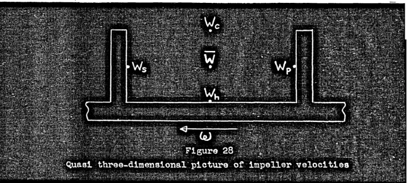
Combining all three solutions results in a quasi three-dimensional solution which gives a clear physical understand-ing of the main flow in the impeller channel.

The design method is completely analytic and all calcu-lations may be made by a digital computing machine.

Thesis Supervisor: Ascher H. Shapiro

Title: Professor of Mechanical Engineering

PREFACE

In writing this thesis, I have tried to keep in mind the need for a simple impeller design method suitable for designers with no more than four years of formal engineering training. However, calculus has been used extensively. Mathematics is such a powerful tool that any designer worth his salt should be willing to sit down with pencil, paper, and eraser and

cal-culate before he begins to specal-culate.

The model of the flow has been based on the one-dimen-sional approach in order to give a clear physical picture of what is going on in the impeller channel. This means that impellers designed by this method will not be the best impel-lers it is possible to make -- they must be regarded only as first approximations which are to be modified after perfor-mance tests have been run.

My first acknowledgment is to Professor Ascher H. Shapiro, my thesis supervisor, who has generously donated his limited time and unlimited talents in maintaining the technical accu-racy and readability of this work. For her accurat~ typing, I wish to thank Dorothy Mastrorillo. Caterpillar Tractor Co., Peoria, Illinois, has generously provided both the leave of absence and the financial arrangements which were necessary that I might devote fUll time to graduate study. Finally, and most important, I express my appreciation to Donna, surely the most patient and understanding of wives.

s

TABLE OF CONTENTS

Literature survey with comments. • • • • .

.7

Flow along the mean streamline •••••••••

Iq

Property changes normal to the mean streamline .'2.0 Property changes from blade to blade • • • • •

.al

Design procedure for a compressor •••••••

2l

SUGGESTIONS FOR FUTURE ,.,ORK ••••••••••• ,," APPENDICES • • • • • • • • • • • • • • • • • • • •

l.7

• • • • • • • • • • • • 7

.. 7

• •• 15

••••

18

• • • .18

.

.

.

.

• • • • • • • • •

.

.

.

.

.

.

. . .

.

. .

• • • • • • • Need for a design method

Units and dimensions

List or assumptions

INTRODUCTION • • • • • • •

:EXPLANATION OF THE DESIGN l-1ETHOD I.

A.

B.

C. II.

A.

B.

C. D.

E.

III. IV.

A Motion of a particle in an accelerating

.2.7

.31

.'1-'

• • • • • • • • • • • • reference frame

Vectors in general curvilinear coordinates ap in cylindrical coordinates, r, ~, and z Derivation of Lorenz's equations for forces

on a fluid particle with axial symmetry ••

52.

B C D

E Lorenz equations for impellers with

straight radial blades _{• • • • • • •}

...

58

F Change in relative velocity normal to a

streamline

.

. . .

.

.

. . .

. .

.

.

. . . "lo

G Control surface analysis in an

TABLE OF CONTENTS

Page H Euler's pump and turbine equation •• _{• •}

.• "\0

J One-dimensional isentropic flow of a

perfect gas along a relative streamline in a compressor or turbine impeller with

straight radial blades and axial

symmetry _{• • • • • • • • • • • • • • •}

.• 95

K Change in fluid properties normal to the

mean relative streamline •••••••••

loq

L Properties at the impeller inlet •• • • • •

It5

M Numerical example - compressor impeller •••

'2\

N Blade surface velocities

v.

REPERENOES _{• • • • • • • • • • • • • •}

..

. . . . I

'7~

• • • • • I~3

I.

INTRODUCTION

A. Need for !! design method

The ability of centrifugal compressors and centripetal turbines to handle a large pressure ratio in a single stage is being eXploited fully at the present time. Small ~as tur-bine engines for road vehicles and helicopters appear to be the most promising applications. At high pressure ratios, compressor and turbine impellers are highly stressed and the trend has been toward impellers with straight radial blades. Radial blades have no bending stresses due to centrifugal force and straight blades are the least expensive to manu-facture. I believe that this trend will continue and that the ma30rity of the small gas turbine engines of the future will use single stage impellers with straight radial blades.

It is for this reason that a simple, rapid, design method for determining hub and casing shapes for centrifugal compressor and centripetal turbine impellers with straight radial blades will be a valuable addition to the turbomacb1nery literature. B. Literature survey ~ comments

The following is a list of those published books and

papers relating specifically to compressors and turbines which I have found to be the most useful in writing this thesis. Reference

3-

"Steam and Gas Turbines" by Stodola

This is certainly a classic and is the logical starting point for any investigation in the turbomachinery field. The Lorenz axial symmetry analysis, basic to most impeller design methods, is developed on pages

990

and

991.

Reference 4- "A Rapid Approximate Method for the Design of Hub-Shroud Profiles of Centrifugal Impellers of Given Blade Shape", NACA TN 3399.

This reference presents a graphical design method which requires about 40 hours for a solution. The flow is assumed to be isentropic, steady, non-viscous, and compressible. The method consists in specifying a blade shape, hub shape, and hub velocity distribution and then drawing, by experience, a streamline adjacent to the hub. The analysis of reference

7

is used to oompute the velocity and density along the assumed streamline. The one-dimensional oontinuity equation, based on the velocity and density at the midpoint of the streamtube formed by the two streamlines, is used to check the mass flow along the streamtilbe. If the mass flows at eaoh station are not equal (within prescribed Umi ts), a new streamline is assumed and the process is repeated. The final streamline beoomes the base line for a new sireamtube. The casing shape is determined by the streamline which finally passes the design mass flow.

The method was used with 3, 5, and 9 stream tubes and it was found that more than 3 streamtubes did not appreciably af-fect the resulting casing shape. This result leads me to believe that using just 1 strearntube (the basis of this thesis) will re-sult in acceptable hub- and casing shapes with a speoified velo-city distribution along the mean streamline. Also, the method of this thesis can be set

up

for a digital computer and

40

hours of hand calculations and graphical measurements are eliminated.

Reference 5- ::A Rapid ApproX1ma"te Method for Determining Veloc1~y Distribution on Impeller Blades of Centrifugal Compressors", NACA TN 2421.

This reference presents a method for compu~1ng o~aae surface velocities after the lmpeiler ~a completely designed. The method is essentially an extension of that aiven in Ap-pendix D of reference

7.

The effect of slip is included here but not in reference

7.

It was shown in reference 4 that in-eluding slip did not appreciably affect the casing shape but did affect the blade surface velocities. However, ne~lectin~

slip is conservative as the blade loading is decreased by slip (good), as shown in reference 4.

Reference

6-

"A General Theory of Three-Dimensional Flow in Subsonic and Supersonic Turbomach1nes of Axial, Radial, and Mixed Flow Types", NACA TN 2604. Wu's analyses and design methods are the most comprehensive that I know. He treats the flow as being 3 dimensional in the analyses and as quasi-3 dimensional in the design methods. His methods would yield very accurate hub and casing shapes but are so iong and complex that, as far as I know, no one uses them.

Reference 7- "Method of Analysis for Compressible Flow Through Mixed-Flow Centrifugal Impellers of Arbitrary Design", NACA Report 1082.

The analysis developed in this reference is the basis of the most recent NACA publication on impeller design (refer-enoe

4).

The analysis can be applied to any impeller with

radial blade elements (the blades are otherwise arbitrary). Appendices B, 0, and D develop equations for pressure and velocity variations from hub to casing and from blade to blade for these arbitrary blades. These equations reduce

to the equations presented in this thesis when straight radial blades are used.

Reference 14- IITwo-Dimensional Oompressi ble Flow in

Oentri-fugal Oompressors with Straight Blades", NAOA Report

954.

This is

an

early

(1949)

analysis of compre~sible,

non-I:

viscous, steady, isentropic flow which is assumed to lie on ."

the surface of a cone. The flow is assumed to,be uniform normal to the cone (from hub to casing). This reference derives the commonly used slip factor equation:

f_s

=

1-+

where

Z

is the number of blades at the outlet.

Reference

15-

naome Elements of Gas Turbine Performance",

paper presented at

SAE

meeting, March

6-8, 1956.

The centrifugal compressor and centripetal turbine ap-pear to have a bright future in small gas turbine engines, such as engines for road vehicles. This reference presents a clear, detailed discussion of gas turbines in general and gas turbines for road vehicles in particular.

Reference

16-

"Approximate Design l-rethodfor High Solldi ty Blade Elements in Oompressors and Turbines", NACA TN 2408.

The design method developed here leads to a blade shape for a prescribed surface of revolution about the axis of ro-tation and prescribed blade surface velocities. It does not determine the hub and casing shapes. The method may lead to blade shapes which are not acceptable for high tip speeds. Reference 17- "Some NACA Research on Centrifugal Compressors",

ASME Transactions, 1953.

A concise resume of the extensive work done by NACA up

&.nd

to 1952Acovers inducer, impeller, and diffuser research. It is an extremely valuable summary of all phases of com-pressor research by the leading U. S. agency in this field. Reference 18- ttTheoretical and Experimental Analysis of

One-Dimensional Compressible Flow in a Rotating Radial-Inlet Impeller Channel", NACA TN 2691.

An excellent discussion of one-dimensional flow in a rotating channel. Effects of friction, choking, and shock formation are included. The effect of losses was found to be similar to the effect of a reduction of flow area. The losses in a rotating channel were placed in four catagories:

1. Friction loss due to the viscosity of the fluid. Friction loss is proportional to the square of the relative velocity and increases rapidly with flow rate.

2. Incidence loss due to a sudden enlargement or contraction of the inlet flow area. Incidence loss occurs at flow rates different from the design flow rate. At flow rates lesa than design, the situation is as shown by Figure A.

The actual flow area Al 1s less than the geometric flow area Al' and a sudden expansion loss occurs as Wl decreases sUddenly to the value Wl'. This loss is proportional to the product

12.

W 2 1

-

_2g o 2 (1 - A fA I) 1 1

and is approximately constant at all flow rates less than

design because _{Wl and Al both decrease.} At flow rates greater than design the situation is as shown by Figure B.

The aotual flow area Al is greater than the geometric flow area Al' and a sudden oontraotion loss oocurs as Wl inoreases suddenly _{to the value Wl'.} This loss is propor-tional to the produot

Wl2 2

1

--- (1 - A '/A )

_2g

o 1 1

and increases rapidly as the flow rate exceeds design because Wl' and

Ar

both increase.

3.

Blade loading loss due to boundry layer separa-tion and secondary flow on the blade surfaces. This loss de-creases as the flow rate is increased because the greater momentum in the main flow delays boundry layer separation.

4.

Shock loss when operating in the range of super-sonic relative velocities. This loss occurs at large flow rates if the static pressure at the channel outlet is too great for completely supersonic flow to the outlet.

Reference 19- "Centrifugal Compressors"

Reference 20- "Design of Radial Flow Turbines"

For complete, up to date information on centrifugal compressors and centripetal turbines, I recommend references 19 and 20. These references are the most complete that I know.

Units and dimensions

Seven independent physical units of measure are used in this thesis:

1. Force measured in pounds of force, lbf 2. Mass, measured in pounds of mass, Ibm

3.

Length, measured in feet, ft 4. Time, measured in seconds, see

5.

Heat, measured in British thermal units, BTU

6.

Temperature, measured in degrees Rankine, R

7.

Angle, measured in radians, rad

As the equations derived in this thesis are valld only in Newtonian reference frames (inertial or accelerating) and thus relatiVity and nuclear reactions are excluded, we may use Newton's second law of motion to relate the first four of the above units of measure:

F

=1iA

80

where F is the unbalanced force acting on a system of fixed identity, lbf; M is the total mass of the system, Ibm; a is the acceleration of the mass-center of the system, ft/sec2; and

50

is a constant of proportionality whose numerical value must be determined by experiment. It has been found by countless experiments that a one potind unbalanced force when acting on a mass of 32.174 Ibm will produce an accelera-tion of one ft/sec2, 1rregardless of the location where the

experiments are performed. Thus, Newton's second law may be written

1

lbf -

32.174 1bm

x 1ft/sec

2

go

1 - 32.174

lbm ft/sec

2

lbf •

80

g , being really equal to the, pure number unity, may be o

introduced int~ any equation to cancel units, whether Newton's law is used or not and, indeed, if motion is involved or not.

Similarly, experiments by Joule and others have shown' that, in Newtonian reference frames, heat and work are related by Joules law:

Q,

=-J-where Q is the heat flowing into a system of fixed identity, BTU; W is the work flowing out of the system so as to maintain the system at its initial temperature, ft lbf; and J is a con-stant of proportionality whose value is determined by experi-ment. Again, countless experiments, irregardless of location, have shown that one BTU of heat flowing into a system results in

778.2

ft lbf of work flowing out of the system to maintain the temperature of the system constant. Thus, Joules' law may be written

1 BTU=

778.2

ft lbf J

J, like

60,

is really a pure number having the value unity, and may be introduced into any equation to cancel units, whether heat 'or work is involved or not.

II. FXPLANATION OF THE DESIGN }iETHOD

A.

.t.1.Ji1 2t as

s\lIUptions

The design method presented in this thesis is based on the following assumptions:

1. The impeller has straight radial blades.

2. The impeller rotates with constant angular velocity about a fixed (Z) axis.

3. The fluid flowing through the impeller is a perfect gas with zero viscosity.

4.

The flow wi thin the impeller has these characteris11cs: a. It may be represented by a mean streamline

which follows the apprOXimate geometric center of the impeller channel.

b. It is isentropic, that is, there is no heat transfer and the flow is perfectly reversible.

c. It is irrotational, that is, its total energy is constant both along the mean streamline and normal to the mean stream-line.

d. It is steady, that is, values of flow

properties at a fixed point in the chan-nel do not change with time.

e. It is axisymmetric, that is, values of flow properties are the same in all meridional

(axial-radial) planes.

5.

Gravity effects are negligible.

6.

The absolute acceleration of the earth with respect to the fixed stars is negligible.

B. Flow along the ~ streamline

It is well known that the relative flow in an impeller channel, although steady, is three-dimensional in nature. Fluid properties vary with distance in all three coordinate directions. The solution of a three-dimensional flow is extremely complex (reference 6) and, for engineers with no more than undergraduate calculus, practically impossible.

It is for this reason that one and two-dimensional approxi-mations are commonly used.

The one-dimensional approximation, that is, assuming that the rates of change of fluid properties in all direc-tions other than along a streamline

are

negUgi ble compared with the rates of change along the streamline, has several

extremely important advantages. Simply and rapidly, it yields results which are valld in the engineering sense and which present a clear physical understanding of the signifi-cant features of the flow.

Using the one-dimensional approach, we assume that the flow in an impeller channel is characterized by one particu-lar streamline, which we call the "mean" streamline. Values of fluid properties along the mean streamline are assumed to be the mean values from hub to casing and from blade to blade.

This assumption, to be valid, restricts the position of the mean streamline -- it must lie (approximately) along the

centerline of the channel.

Appendix J presents the results of a one-dimensional analysis of impeller relative flow, within the assumptions presented previously. Using these results (collected in

Table 1), we specify, by experience or by fluid mechanics theory, a velocity distribution along the mean streamline. If this distribution is linear with radiUS, or constant, the required flow area at any radius is computed in closed form, as shown in Appendix

J.

otherwise, numerioal integration

must be used. All channels having this calculated area-radius r~lationsh1p are equivalent as far as the one-dimensional

analysis is concerned. We must turn to a two-dimensional analysis to select one particUlar channel from the infinite number whioh are satisfied by the calculated area-radiUS relationship.

c.

Property changes normal .~ ~ ~ streamline

Table 2, in AppendiX K, presents the results of a one-dimensional analysis of property changes normal to a relative streamline. By combining these results with those summarized in Table 1, we have a quasi two-dimensional solution of the flow in the meridional plane, since, with straight radial blades and axial symmetry, the mean streamline must lie in this plane. This quasi two-dimensional solution enables us to select the one particUlar channel which fulfills our design

requirements (such as space or weight limitations or the need for highest possible efficiency). The selection is ac-complished by assuming a mean streamline and then computing the corresponding hub and casing profiles and velocities. If these profiles or velocities are unacceptable, a new mean streamline is assumed and the calculations are repeated.

Originally, I had planned to develop a design method in which the hub and casing velocities are specified and the corres-ponding hUb, mean streamline, and casing shapes are computed. This procedure was found to be unacceptable as the calCUlated mean streamline would not, in general, 11e on the (approxi-mate) centerline of the channel. In the proposed method,

all oomputations may be done on an automatio computer and, for a fixed set of design parameters, several .assumed mean streamlines may be fed into the oomputer and the designer (or teohnician) merely plots the results. This procedure also gives a olear picture of the effects of mean streamline shape on the flow in the meridional plane.

D. Property changes from blade to blade

Having an approximate picture of the flow in the meridio-nal plane, we use the analysis of AppendiX N to compute pro-perty variations from blade to blade. These variations are intimately associated with the number of impeller blades and the analysis of Appendix N helps us to understand the influence of blade number on blade loading and behavior of the boundry layer.

By

combining the two-dimensional meridional plane

solution with the one-dimensional blade to blade solution, we obtain a quasi three-dimensional solution throughout the

entire impeller. Thus, with the aid of this quasi three-dimensional solution, we can evaluate the gross effects of hub shape, casing shape, and blade number on size, weight, and efficiency.

E. Design procedure f.Q.!: 1! compressor A. Preliminary steps:

1. Specify the properties of the perfect gas which is to be used

a.

Inlet stagnation pressure and tem-perature

b. Outlet stagnation pressure c. Mass flow

d. Ratio of specific beats e. Molecular weight

2. Compute the following: a. Tip speed

b. Casing radiUS, tip radiUS, and angular velocity

c. Hub radius for known (or assumed) blade number and thickness at in-ducer inlet

d. Properties at the inducer inlet e. Properties at the impeller inlet,

including the radius to the mean streamline.

B. Hub and casing design:

1. Specify the relative velocity distribution along the mean streamline

2. Using the analysis given in Appendix J, compute the corresponding area distribution normal to the mean streamline at specified stations on the mean streamline

3.

Specify the shape of the mean streamline (its angle with the Z axis) and compute its radius of curvature at all stations

4.

Divide the areas computed in step B2 into two parts -- one area extending from the hub (as yet undetermined) to the mean streamline, the other area from the mean streamline to the casing (also not yet determined). This step is neoessary to be certain that the mean stream-11ne will 11e approximately midway between the hub and casing

5.

Using the angles specified in step B3 and the areas of' step B4, compute the hub and casing radii at all stations. The hub and oasing are now completely determined.

O. Evaluation of the hub and casing design:

1. Using the mean streamline velocities specified in step Bl, the radii of curvature of the mean streamline computed in step B3, the hub and casing radii from step B5, and the analysis of

2.

Appendix K, compute the hub and cas-ing relative velocities at all stations. 2. Plot the results of steps B3 and 01. On

the basis of space or weight limitations and boundry layer theory (or experience) evaluate the hub and casing design. If unacceptable, repeat the design, begin-ning with step B3, until satisfactory

shapes and velocities are produced. This completes the design in the meridional plane.

D. Ohecking blade loading 1. Using the following:

a. Properties at the impeller inlet from step A2e

b. Velocities along the mean streamline from step Bl

-c. Areas normal to the mean streamline from step B2

d. Mean streamline angles from step B3 e. Known (or assumed) blade number and

thickness at all stations f. The analysis of AppendiX N, compute the blade surface velocities.

Plot the results or step

DI.

On the basis of boundry layer theory (or experience) evaluate the choice of blade number and

thickness made in step Dle. If unaccept-able, repeat the design, beginning with step Dle until satisfactory velocities are produced. Since blade number and thickness have only second-order effects on the hub and

casing shapes, it is not necessary to redesign the hub and casing until step D2 is considered satisfactory. The final design is then made, beginning with step A2e.

III. SUGGESTIONS FOR FUTURE WORK

Time limitations prevented my working out a detailed turbine design. The equations developed in this thesis are based on first principles and are valid for turbines as well

as compressors. The details

or

design, however, will be dif-ferent. The flow enters a turbine impeller after leaving a

set of nozzles (rather than an inducer) and leaves the impel-ler by entering an exducer (rather than a diffuser). Thus, the leaVing flow must be analyzed, rather than the entering flow as was done in AppendiX L. Centripetal turbine design methods are even more scarce than compressor design methods

and I hope that this thesis will be the starting point for a similar detailed turbine design.

IV.

APPENDICES

Anpendix A

ap vector absolute acceleration of P i

j unit vectors in the x, y, z directions

K

0A origin of accelerating reference frame 0I origin of inertial reference frame

P a particle of fixed identity mOVing in any manner in an accelerating reference frame

R_A position vector or P from 0A RI position vector of P from 0I

He

position vector or 0A from 0I

tA time as measured in the accelerating reference frame t

I time as measured in the inertial reference frame V_p vector absolute velocity of P

W vector relative velocity of P ~

Wy scalar components or

W

in the x, y, z.directions ~

~

Y_A orthogonal directions defining an arbitrarily ac-ZA celerating reference frame

XI

Y₁ orthogonal directions defining an inertial reference ZI frame which is fixed in outer space

x

y instantaneous scalar coordinates of P with respect to z 0A in the XA YA ZA accelerating reference frame V vector operator defined by equation (16)

~ vector absolute rotation of the accelerating refer-ence frame

c.>x

'-'y scalar components of (u in the x, y, z directions

Wz

Appendix A

MOTION OF A PARTICLE

IN AN ACCELERATING

REFERENCE

FRAME

XI

Y

₁

ZI determine an orthogonal inertial referenoe

frame, fixed in outer sRaoe (~

fixed to the earth).

X

_A

Y

_A

ZA determine an orthogonal referenoe frame,

!.£-oelerating in any manner with respeot to the inertial (I)

frame.

P is a particle moving

in

any manner in the acoelerating

(A) frame and instantaneously located at the point (x,

y,

z)

in

the A frame.

If

I

is the position vector of P with respeot to

_°1.

irA

is the position vector of P with respeot to

_°A.

Ir

_o

is the position vector of 0A With respect to 0

₁

•

1,

1,

and

E

are unit orthogonal vectors

in

_{the XA, YA,}

ZA directions.

1,

1,

and

it

are constant

in

magnitude

!!!A

direotion

in

the A frame.

In general, they are constant

onll

.!!!

IIl!Snitude

in

the I frame sinoe the A frame may be

rotating with respect to the I frame and,

in

that case, the

direotions of

1, "j', and

1t

would be ohanging

in

the I frame.

From Figure 1,

The derivative

01' ~

with respect to time

in

the I frame is

the velooity

ot

P

in

the I frame (the uabsolute" velooity

01' P),

V

_p•

(1)

From Figure 1,

irA

=- 'IX

+

1y

+

Kz

Differentiating

(2),

em

-'A

=

'I

dx + di x +

:r ~

+ dJ y +

K

dz +

d1t

z

o:tI

o:tI o:tI

a:tI

o:tI

o:tI o:tI

Grouping terms,

:AI

=

rr ~

+

1

H:

of.

K ~

]

+

rfi

x +

!f

Y

+

ff '

z]

I

I

I

I

I

I

(:3>

Since x, y, and z are scalars, they have identical time

deri-vatives

in

both the

I

and

A

frames.

The

first bracket in

(:3)

may be written:

[1' dx

+!.9Z....

+ K d.z ] = [1 dx

+! ~

+ K dz] (4)

<rtI

C!tI

a:tI

<itA

CItA

<itA

The derivatives of the unit vectors

in

the second bracket of

(3) are perpendicular

to these vectors and may be written:

31

dl

--~-ldk-~

dE:

=

/I.J

xi,

a:;:;

=

tV

x

, erE': •

lJ) X £.

I I I

(5)

where

{jj

is the vector rotation

ot the

A

frame with respect to

the

I

frame.

(6)

Expanding

(5),

we have, using

(6),

~

-

-o;c:

I: k (f)x - ilV

z

I

Combining

(3), (4),

and

(7):

alt

A

I

dx -r

.&-.

~

dz

'dt:

= [ dt + J dt + K

dr]

I :A :A 'A (7a) (7b) (7c)

+

[-ltltJ_y

x

+ jW

_{z x}

+

Itw

_x

y -

'rlJ)z

Y - jW

_{x z}

+

"I'W

_y

z]

(8)

<il!

The first braoket of (8) is the expansion ot

dt~'

the

velo-oity ot

P in

the

A

frame (the "relative

ll

_{velooity of}

_p),

sinoe

I,

I,

and

k

are oonstant in magnitude and direotion

in

the

A

frame.

The second bracket ot

(8)

is the expansion of

W x

R

_A.

Inserting these equivalents into

(8),

we have:

.32.

Combining (1) and

(9):

_ dill

dR

o dRA _

V

p :=I ~ •

dt':' ...

dt

+

W

x

lt

A

I I :A

(10)

From

(9)

we see that the derivative of any vector in the A

frame with respect to time in the I frame is equal to the

deri-vative of that vector With respect to time

in

the A frame plus

the vector product of that vector With

W.

We now make use ot

this fact in differentiating

V

_{p to obtain}

ap,

the acceleration

of P in the I frame (the absolute acceleration of

pl.

From (10),

dR'A

rw

x

dt:'"]

:A

From

(9),

the second bracket

ot

(11) is:

dztr

= (

:A]

+

dt2

_'A

(11)

Detining the relative velocity of P as

W,

the first bracket

ot

(12> is:

Since

W

is the relative velocity of a particle of fixed

identity, we use the special notation capital D to denote sub-stantial differentiation while following the motion of this particle.

V

is a function of space and time (x, y, z, and t

A), thus:

But, ~ , ~, and ~ are the scalar component s

ot 'l

in the

A A A

x, y, and z directions, respectively.

(15) may be written in more compact form by introducing the vector operator,9. In x, y, z coordinates,

33

(16)

'i151==

(lWx+JWy+kwz>'Cr1x+l-fy+i

tz>

== W_x

tx

+ W_y

-fy

+ Wz : z (NOTE:

'i1

51 ~ V.

'1)

Thus,

(15)

may be written,

~: (t:Y' ~) f:l"

dW'

UUA n. v n

+~tA

The seoond braoket of (12), trom (13), is:

dJt

- 'A_ - t:P

fA)

x dt

A

=

W

x

n

The third braoket of (12), trom (13), is:

d - ;=:0) - a

dW

~

'd."t7

«(U

X l\A

=

W X " +

n:-

X l\A

A

A

Introduoing (12), (13), (18), (19), and (20) into (11):

d~

aw

a:...

s [ 0] + [(w •~ )

W'

+

~J

.t' ~ ~A I

(18)

(19 )

(20)

(21)

(21) is the basio kinematic equation of motion of a particle

moving in any manner in a reference frame (the A frame) which

is itself accelerating

in any

manner With respect to an

inertial frame (the I frame).

In words, the absolute

accelera-tion of P equals the absolute acceleraaccelera-tion

ot

the origin

01'

the

A frame (first bracket) plus the total acceleration

of P if the

A trame were not accelerating

(the total acceleration

of P as

of the aoceleration of the A frame)(second braoket) plus the

sum of the tangential and normal accelerations of P about 0A

due to the rotation of the A frame if

P

were fixed in the A

frame (third bracket) plus the nOoriolis" acceleration of P

(fourth bracket).

All of the above was adapted from

refer-enoe

1, p.

249-252.

For our purposes, we consider the inertial frame as being

fixed to the earth, With

01

at the center of the earth.

This

means we are neglecting the absolute acceleration of the earth

With respect to the fixed stars.

This leads to insignificant

errors for the present work since the angular velocity of the

earth is only about

7

x

10-

5

rad per see (reference

1,

p.

269).

Our A

trame is defined as being attached to the surface of the

earth and rotating with an angular velocity

iiJ

about the ZA axis

only.

Thus, ~ has no components in the

_XA

and

_YA

direotions

and

The distance

I

Irol is assumed to be constant and we neglect the

angular velocity of l{o (the angular velooity of the earth).

Thus,

We also assume that ~ is constant in magnitUde, thus

dW

-k dW iii 0

dt7 ::

d't:'"

-~ 'A

Equation

(21) reduces to:

ap

= (If •

V)

V +

lJa.e

V +

i~

x (it

w

x irA) + 2kl.fJ x

W

(22) 'A

Appendix ~ hl

~ lengths or U vectors _{in the ul' ~, u3 directions} h

3 i

3

unit vectors in x, y, z directions

k

0A origin of accelerating reference frame

P a particle of fixed identity moving in any manner in an accelerating reference frame

37

position vector or P from 0A

vectors tangent to arbitrary orthogonal

curvi-linear surfaces at the instantaneous location of P Ul

~ unit vectors tangent to arbitrary orthogonal

curvi-u3

linear surfaces at the instantaneous location of P

scalar coordinates or P in an arbitrary orthogonal reference frame

vector relative velocity of P

x

y

z

orthogonal directions defining an accelerating reference frame

scalar coordinates _{of P in the XA YA ZA} accelera-ting reference frame

vector operator using ul' ~, u3 coordinates -defined by equation (28)

vector absolute rotation of the accelerating reference frame

scalar components of Win the ul' ~, u3 directions

Appendix B

VECTORS IN GENERAL CURVILINEAR COORDINATES

Let ~,

~,

and ~

be any orthogonaJ. curvilinear

co-ordinates which form a right-handed

system.

For example,

x, y, and z

in

Appendix A form a right-handed

system.

If irA

is the position vector of P from 0A'

ItA

:I

1x

+

"J"y

+

KZ

We now define the following:

h

l ;; Itrll

~

;; (TJ

₂

1

h

₃

is

lu

₃

1

11

- - 1

~:lIi1

tf

-

_~:lii:

- 2 2

__

U,

U

3

:I h

3

(23) (2l1e. )

(24b)

(240)

(25a)

(25c)

(26a)

(26b)

(26c)

The

rrls

are vectors tangent to the coordinate

surfaces; the h'S

are the J.engths of the

tr'

s; and the \i's are unit veotors tangent

to the ooordinate

surfaoes.

In these general ooordinates:

(27a) (27b) (28)

hJ.

UJ.

h

2

U

2

_~~ VxV=h

h

1

h

...2-

....a..

-.4.

(30)

J. 2

3

auJ.

~u2

c)u3

h

1

W

l

h

2

W

2 h₃ W₃

Appendix B adapted from referenoe 2,

p. 321-327.

Appendix C ~p vector absolute acoeleration of P

ar

a~ scalar components of ap in the r, ~, z directions

az h_r

'tlg.. lengths of U vectors in the r, -Q-, z directions

h

_z

r

1

k

m

unit vectors in the x, y, z directions

unit vector in the r direction

unit vector in the Q direction

origin of accelerating reference frame

a particle of fixed identity moving in any manner in an accelerating reference frame

RA position vector of P from 0A r

~ scalar cylindrical coordinates _{of P in the XA YA ZA} z accelerating reference frame

tA time as measured in the accelerating reference frame

U

_l

U

₂ vectors tangent to arbitrary orthogonal curvilinear U

vectors tangent to the r,~, z orthogonal curvi-linear surfaces at P

unit vectors tangent to the r, ir, z orthogonal curvilinear surfaces at P

scalar coordinates of P in an arbitrary orthogonal reference frame

vector relative velocity of P

scalar components of

W

in the r, Q, z directions

orthogonal directions defining an arbitrarily ac-celerating reference frame

x

y scalar coordinates _{of P in the XA YA ZA accelerating} z reference frame

V vector operator using r, Q, z coordinates - defined

by equat10n

(45)

~ vector absolute rotat1on of the accelerating refer-ence frame

-scalar componentsof W in the r, -Q-, z directions

w

resultant scalar componentof

W -

defined by

AppendiX C

ap

IN CYLINDRICAL COORDINATES,

r,a,

AND

z

We reter to Appendix B for the equations for

u,

~A'

W,

h,

From (23), Appendix B,

irA ==

'Ix

+ "'j'y +

i'z

From Figure

3,

x.;;

IIxI==llrl

oos

e

=

r oos

e

y ~

111

I

a IIr

I

sin

e

:I r sin

e

Introduoing (31) and (32) into (23),

irA ==

'Ir

oos

e

+ Jr sin

e

+ KZ From (248), Appendix B, and (33),

. ()If

... -U

-

'A - -r u₁I: r ==

0

r • i oos

e

+ J sin

e

From

(34), (31)

and

(32),

U' ==

1" ~

+

J

:t.

== ];

('Ix

+

Jy)

r r r r From Figure

3,

Ix

+

1y

=£r

From

(35)

and

(36),

-tr

_r ==-R-From

(24b)

and

(33),

(34)

(35)

(36)

(37)

45

From

(38), (31),

and

(32),

. ~

From Figure

3,

From

(39)

and (40),

From

(240)

and

(23),

-iy

+ jx

=

mr

(40) (41) (42)

From (25), (26),

(27),

and (28)

in

Appendix B, and from

(37),

(41), and (42),

~ =

lt1

r

I

== 1

he

a

IU

_e

I=

r h_z

=

I

_t1z

I

= 1

-w

=

.£

lIJ

_r

+

'in

we

+

i'

W

_{z ;;}

1t

fA)

v=l

..L+:!

..L.+i'L...

tJr

r

aa

~z

(44)

(45)

We now expand

ep

in

r,

a,

z coordinates.

From AppendiX A,

equa tion (22),

We expand the terms

in

(22).

From

(43)

and

(45),

-W' •

9

a (/. W +

iii

W

_a

+

i'

w )

r

z

-

-

1z

~

W

a

_d

• (1,

.L

+!!

-2...

+

it

) :::

W -

+..1L

-a

8

+

W

_z

~r

r

08 .

z

r clr

r

dZ

(47)

Before expanding

(47),

we notice that all partial derivatives

-of the unit vectors.t ,

'iii,

and

it

with respect to the r,

e,

z,

coordinate directions are zero because the unit vectors are

always

ot unit J.engthand orthogonal.

1.

and

in

rotate about the

Z axis as P moves

in

the A frame and these rotations will

pro-duce partial derivatives with respect to time, as we shall see

later.

Returning to

(47)

and using

(43),

- a

W

_r

c)w

_e

a

w

_z

(W • \1)

W'

=

w

_r

(I. ~

+

in

ar

+

It

ar-)

we -

~w

~we

aw

+

r

(R, 0

e

r

+

Iii

Ta

+ It lJ

e

Z)

48

(48)

0'1 Expanding

a

t A and using

(43),

o'iT .

lowr

at

-

aWe

a

iii

ilA::r

atA

+

~tA W

r + m ~

_{+ c)tA We}

(49)

: ~ a t1me rate of change of

I

in the A frame

=

iii ~

where

'iii

gives the direction of the change (normal to

1

and in W

the positive

e

direction) and r

e

is the instantaneous angular

-velocity

ot

i

(and

iii)

about the Z axis. Thus,

01

= m~

() A r (SO)

~-

-w

Similarly, at~

= -.£

r

e

where

-I,

gives the direction

ot

the change (normal to

Iii

and in the positive

e

direction). Thus,

(51)

Thus,

~k

0 (}t;' = A

Combining

(49), (50), (51),

and

(52),

(52)

(53)

Expanding ~(J)x

(i:w x

R'A)'

we have, using

(33),

klaJ

x

[it'w

x

(11'

cos

e

+

1'1'

sin

e

+

k'z)]

=

klU

x

<:r

w.r

cos

e -

l'

caI,r sin

e)

=,.,2

(-Tr

cos

e -

Jt"sin

e)

Using

(54),

(31), (32) and (36),

Expanding

2"fW

x

'I,

we have, using

(43),

Combining

(22),

~),

(53), (55),

and

(56),

(54)

(55)

+ W Z

on

aW

d

W

_e

aw

ap ::

r

W

_r

(~#

₊

_{Iii 0 r}

_{+ 1t}

a

_{rz )}

-

oW

r

_

aWe

_

qW

z

(I.

as

+ m

'd""6

+ k (J

e )

,ii

oW

_r

_

aWe

_

aw

_z)

~dZ+maz+kaz

50

(57)

The ~irst bracket

1n

(57)

is the relative acceleration ot P

(if the A frame were not rotating), the second bracket is the

-centripetal acceleration of P due to the rotation of the A

frame, and the last bracket is the Corio1is acceleration of P,

also due to the rotation of the A frame.

Equation

(57)

is the kinematic equation of motion of a

particle of fixed identity moving

in

a rotating reference

frame under the following conditions:

1.

The inertial reference frame is attached to the

surface of the earth with its center at the center of the

earth.

We neglect the angUlar velocity of the earth.

2.

The origin of the rotating reference frame remains

a constant distance from the center of the earth.

3.

The rotating reference frame rotates with constant

angular velocity about the

'Z

axis.

We may write

(57)

in scalar form in the r,

a,

and z

directions:

oW

_r

we

oW

_r

.

dW

oW

r +

r

a

=W

-+-

_n-+

_Wz

r

r Dr

r

~z

a

t

_A 2

We

2

(S7a)

- - -IJ)

r -

2f1JW

r

e

(}W

_e

We

aWe

o

We

~We

a

_e

=W

_{r c)r}

-+-

_r

_~

₊

_W

_z

_dz

₊

_7tA

W

W

+ e

r +

21JJ'd

_(57b)

r

r

oW

_z

We

OW

z dWZ dWZ

(570)

az

=

w

_r

ar-

+

r

78+

W

_z

_()z

₊

av:-A

Sf

Appendix

I!

scalar accelerations of P in r, -Q-, z directions,

ft/sec2

distributed body forces per unit mass in the r, """,z directions, lbf/lbm

p

o

universal constant relating force and mass,

. 2

32.174 Ibm ft/sec Ibf

origin of accelerating reference frame a particle of mass of fixed identity, Ibm

static pressure exerted by other fluid particles on P - in positive r direction, lbf/ft2

Pz static pressure exerted by other fluid particles on P - in positive z direction, lbf/ft2

p static pressure, Ibf/ft2 (for non-viscous fluids, p

=

Pr

=

_Pz

=

same in all directions at a given point in the fluid)

R force exerted by o~her fluid particles on P - in positive r direction, lbf

R' force exerted by other fluid particles on P - in negative r direction, lbf

a

force exerted by impeller blade on P - in direc-tion of

<v,

lbf

a'

force exerted by impeller blade on P - in direc-tion opposite to W, Ibf

z

Sr

S~ components of S in the r, -9-, z directions, lbf Sz

Sr'

S ' components of S' in the r, ..g., z directions, lbf

:Q-S I

Z

force exerted by other fluid particles on P - in positive z direction, lbf

Z' force exerted by other fluid particles on P - in negative z direction, lbf

~ static density of P, lbm/ft

3

~ angular velocity of accelerating reference frame about Z axis, rad/sec

Appendix D

DERIVATION

OF LORENZ'S

EQUATIONS

FOR FORCES ON A

FLUID PARTICLE

WITH AXIAL

SYMMETRY

We shall use the Lorenz axial symmetry assumption (reter-ence

3,

p.

990-991)

to derive the forces which cause P to ac-celerate. We will derive these equations tirst for a compressor.

In Figure

5,

ABCD

and

A'B'C'D'

represent adjaoent im-peller blades an infinitesimal distanoe, rde, apart. The blades are infinitely thin and there is an infinitesimal mass of flUid, P, between the blades. The blades exert forces S and S' on

P,

8 from

ABCD

_{and 8' from}

A'B'C'D'.

We now assume

P

has ~ viscositl, thus 8 and 8' act normal to the blades. 8ince the blades, in general, are warped, S and 8' will have oomponents in the coordinate directions. We call these com-ponents _8r,

Se'

8

_z'

Sr',

_Se',

and SZ'. The fluid outside of the blades also exerts forces on

P

at the open edges

ABBIA',

DCCIDI, BCC'B',

and

ADD'AI.

We call these fluid forces

R, RI,

Z, ZI,

respectively. We now define: 8 - S I r r P

S

- Se

I

Fe

-

e

e

_P

Sz

-

SzI

Fz

-

_P

F

_r,

Fe'

and

F

_z

are called the "distributed body foroes per unit mass" in the coordinate direotions. We can now write the Lorenz equations:

S5

- P

PF

+ R - RI

= ---

a

PF

+

Z - Z.

=

E-

a

z go z

From Figure

5,

as P approaches zero, p

=='t

dr rd8dz R =t Pr rdEldz Z =t Pz dr rd8 (58b) (58c)

(59a)

(59b)

(59c)

(S9d)

(5ge)

Since we have assumed that P has zero viscosity, as P approaches zero, p

=

p

=

p (hydrostatic state of stress).

r

z

Combining

(58)

and

(59),

we have, after cance1lation,

'" F_"z

-..£.:R. -

_{az - g}

1-

a_z o

( 6oa)

(6Ob)

(600)

The equations for a turbine are different only in sign. Our coordinate system is as follows:

I

I

We see that~,

e,

and

Z

are reversed while r remains the

same as before.

Our blades now look like this:

Our definitions of

R, RI, F

_r

,

Fe'

and

F

z are unohanged.

We change the direction of Z and ZI.

Z now acts on surface

ADDIAI

and ZI now acts on surfaoe BOGIBI.

The Lorenz

equa-tions for a turbine are then identioal with those for a co~

pressor (equations (60) ).

Appendix E

D indicates substantial differentiation while following a particle of fixed identity

Fr

F.g. d1stributed body forces per unit mass 1n the r, ~, z F

z direct1ons, lbf/lbm

58

p

z

universal constant relating force and mass, 32.174 Ibm ft/sec2 lbf

static pressure, lbf/ft2

scalar cylindrical coordinates of a particle P mOVing in an accelerating reference frame

radius of curvature of the relative streamline along which P moves when P is at the point r, -Q-, z; ft

s

n scalar streamline coordinates of P when P is forced to move in the meridional plane

t

A time as measured in the accelerating reference frame, see

W

_r

Wg scalar components of W in the r, g, Z directions, ft/sec

Wz

Wm scalar component of W in the meridional plane, rt/sec (for impellers with axial symmetry and straight radial blades, Wm

=

W)

~ angle between Z axis and positive s direction (Figure 8), rad

~ static density of P, lbm/ft3

~ angular velocity of impeller about Z axis, rad/sec ~ indicates pa.rtial differentiation while holding all

Append1x E

LORENZ EQ,UATIONS FOR IMPELLERS WITH STRAIGHT RADIAL BLADES

Comb1ning

(60) 1n

Appendix

D

and

(57) 1n

Appendix C

J

we have:

dn

f

oW

_r

We dW

_r

JW

_r

'f

F

_r

- ~_d

_r

= -

_g

(W

_r

-_d

_r

+ - ~..,

e

+ _{Wz ~z} rO'o o 2 dW_r We 2 + -:or- - - - W r - 2 lJ>W

_e)

dllA

r (6la)

(61b)

(61c)

By our assumption ofax1al

symmetry, all partial der1vat1ves

w1th respect to

e

are zero.

By our assumpt10ns of zero

v1s-co

s

1ty and

s

tra1ght radial blade s,

F

r

=

F

z

=

We

=

o.

Equa-t10ns (61) become:

(62b)

(62c)

With straight, radial blades, the particle P is forced to move in the meridional (axial-radial) plane and it is convenient to follow its motion in this plane in terms of streamline co-ordinates, sand n, as shown in Figure

8.

We notice that the parentheses terms in (62a) and (620) are the substantial derivatives ot W

r and Wz' respectively (Appendix A, equation (15) ). That is, since

1e

:r 0,

DW ~W

dW

JW Z

=

w

Z

+

w

--!

+ Z

l>tA

r

7I=

z tJ z

dtA

(631))

We now assume that the flow relative to the rotating impeller

does not vary with time ("steady" flow), thus

aw

~W

at~

==

;Jt: :;

0

From Figure 9c,

Taking the substantial derivative or

(65):

~ :2

-w

sin

01..

DO<

+

DW

cos

I)/.

1)"A

1rnA 1rnA

From Figure 8,

By definition of a streamline

in

steady flow,

Ds _

w

lre7

-~

Dn

-0

D't7

-~

(64)

(65a) (65b) (66&) (66b)

(67 )

(68a) (68b)

Taking the substantial derivative of W,

DW

dW

Ds +

aw

Dn

(69 )

1reA="7S

_ntA7ii

_1reA

Combining ( 67) and (68a):

~

_=1t""'"

W

(70)

'A

0

Combining ( 66 )I (.q8b ), ( 69 )I and (70):

DW_Z' W2 ~W

15i7

= -

lr

sino( + W ~ oosO<

A 0 as

Combining

(62),

(63), and (71):

(7la)

(71b)

d n (,p

w

2

a

w

--.~

- .-...- =

..L.. [w- oos.t:Jt..+ W - sin 0< - W- r] (72&)

ar

go .no

d

S

D CoP W2

aw

- -eR.

I: -1.. (-

Jr"

sine:<.

+

W ~ oosD(] (720)

(}z

go 0 dS

We now find ~; and ~ ~ •

t:Jz

From Figures 9a and 9b,

Combining

(72),(73),

and

(74):

2

W

2

dlf

2

- tIJ

r

sin c.( -

R

sin 0< OOB 0(

+

W

a

s

oos c<.) =t

o

2

w

2 2 dW

+lJJ

r

ooso(-R

o sin o(+W

~s

s1no<.ooso<.)

=

r.p W2 2 - -1.. (-

r

+ W r ooso() go 0 (73b) (74b) (740 ) (74d) (75a) (75'b)

Combining (74) and (75):

(76a)

(76b)

Equations(76) are identical tor a centripetal turb1ne if the

sand

n directions are as shown

in

Figure

9d.

Appendix F

c

_p specific heat at constant pressure, BTU/lbm R C

v specific heat at constant volume, BTU/lbm R go universal constant relating force and mass,

32.174 Ibm rt/sec2 1bt

HA Bernoulli constant for flow along a relative stream-line, ft2/sec2

Bernoulli constant for flow along an inertial (absolute) streamline, ft2/sec2

h static enthalpy, BTU/lbm h

oA stagnation enthalpy defined by equation (110), BTU/Ibm

hoI stagnation enthalpy defined by equation (110a), BTU/Ibm

J universal constant relating work and heat,

k P R s n T u 778.2 ft lbf/BTU

ratio of specific heats, C /C

p v static pressure, lbf/ft2

gas constant, ft lbf/lbm R

radius of curvature of the relative streamline, ft radius from Z axis, ft

streamline coordinates for two-dimensional flow in the meridional plane

static temperature, R intrinsic energy, BTU/lbm

V absolute velocity, tt/sec W relative velocity, ft/sec ~ static density, lbm/ft3

~ angular velocity of impeller about Z axis, rad/sec

Appendix F

CHANGE IN RELATIVE VELOCITY NORJ~

TO A STREAMLINE

We have shown

in

Appendix E that the Lorenz equations

for impellers with straight,radial blades are:

(77a)

(77b)

If we temporarily confine our attention to ohanges along a

partioular relative streamline, (77a) beoomes:

(770)

MUltiplying

(770) by ds and integrating,

-go~

~

-

~2 +

uf2r~

=

oonstant of integration;

_HA

(78)

\,

We see that HA(usually oalled the Bernoulli oonstant of the

streamline) is invariable along the streamline but may vary

from streamline to streamline.

We now investigate ohanges

in

HAnormal to a partioular streamline.

In this oase, (77b)

beoomes:

If we differentiate

(78) with respect to n (at constant

a),

we have:

(79)

But -go ~

S

V

= - ~

~.

so (79) may bs written:

(79a)

Rewriting

(77d):

(?7d)

Subtraoting

(7?d) trom (79a), we see that:

(80)

Now, it HA,the oonstant ot integration

1n

equation (78), is

identioal tor ~

relative streamlines,

it will not vary

in

any

direotion and:

.@A- 0

_ana

It (81) 1s true, then (80) becomes:

dW W

diia-a;

(8l)

Equation (82) gives the rate of change of the relative velo-city in the normal direction, under the condition of

(81).

We now investigate condition

(81).

If the fluid flowing

through the impeller originated in a large reservoir (such as the atmosphere) where ~ :; ~; , we see from equations (77c) and (77d) that ~~ :;

!:::

-

*;,

which is equation (82). Thus,

in a large reservoir, equation

(81)

holds.

Aocording to Kelv1n's theorem (reference

9,

p. 280), equa-tion

(81)

will hold in any region in which three conditions are met:

1. Frictionless flow

2. Conservative body forces only

3.

Density of the fluid depends only on the pressure Condition 1 has already been specified in deriving the Lorenz equations (Appendix D); oondition 2 is satisfied by gravity and centrifugal force fields; and condition

3

is satisfied, for air and other perfeot gases, by the isentropic relation:

70

-k

P'f :::constant

(83)

We now speoify that the f1.ow through our compressor and turbine impe1.lers originates in the atmosphere and also that the three conditions of Kelvin's theorem are a1.ways satisfied. Any flow which satisfies Kelvin's theorem is called "irrotational', and equations (81) and (82) may be used in all irrotational flows.

Equation (8~) ho~ds for relative flo'tofsonly. In an inertial reference frame, the absolute velocity (V) is the ve~ocity "rela-tive" to the frame, thus (81) holds, under the conditions of

Kelvin's theorem. (81) does

E£!

hold for the relative velocity

(li) in an inertia~ frame. Thus, under the conditions of Kelvin's theorem,

11

dHA

a:n-

=

0 in an inertial frame in an aocelerating frame (8lia)

(84b)

where, using

(83),

) 2 2 2 H ;; -g ~ - W + 6) r A 0

'f

r

2 2 2 2 ::f _g (k) Eo _ W + It)

r

o

i=I

'f

r

2

(8Sa)

(8Sb)

HI and H

A are related to the stagnation enthalpy (1I0a) and (\10) in Appendix

G.

To show this re1.ationship, we make use

or

the perfeot gas relat1ons:

B~ c\e.f\n~t.,oh I for a.n~ 5ubstancc,J

h;U+JV

FoW"

a.n

pc\""Fe.c:;-(:; ga,s e";),)

U :: 0 T v

o -

0 :: ~ p V u , P

=i

R T

h ::

0

T

P

From (110 ) and (lIo

a),

_

w

2 fJJ2 r2 hOA !! h +

2g

J -

2g J"""

o 0 2 h ;; h + _V _ 01 2g oJ

Oombining (110), (\loa), (868.), (86b), (86e), and (86t),

(86a) (86b) (860) (86d) (86e) (86t) (86g) (110 ) (lJoa)

72.

2

w2

2 -g J

h

::

-g (A) E. -

!....

+ r

(87a)

o aA 0 k- J.

'f

2 2

We see that (84)

may

be written:

73

in

an inertia]. frame

(840 )

in

an aooelerating frame

os

d1f

dA

Appendix G

a control surface, fixed in a specified reference frame, through which systems flow

a control volume (the space enclosed by a control surface)

an infinitesimal volume element of a control volume, ft3

an infinitesimal area element of a control sur-face, ft2

an infinitesimal area element of a control sur-face through which a system enters the control volume, rt2

an infinitesimal area element of a control sur-face through which a system leaves the control volume, ft2

specific heat at constant pressure, BTU/lbm R denotes substantial differentiation while

follow-74

e E

ing the motion of a system of fixed identity total internal energy of a system, BTU

internal energy of a system, BTU/lbm

internal energy of a system just before the system enters a control volume, BTU/lbm

eout internal energy of a system just before the system leaves a control volume, BTU/Ibm

universal constant relating force and mass, 32.174 lbm ft/seo2 lbf

h

boA

hOA in

boA

out

hol

hoI

in

bol

out J M m

static enthalpy of a system, BTU/lbm

stagnation enthalpy of a system, defined by equation (110), BTU/lbm

stagnation enthalpy of a system Just before the system enters a control volume which is fixed in an accelerating reference frame, BTU/lbm

stagnation enthalpy of a system just before the system leaves a control volume which is fixed in an accelerating reference frame, BTU/lbm

stagnation enthalpy of a system, defined by equation (llOa), BTU/lbm

stagnation enthalpy of a system just before the system enters a control volume which is fixed in an inertial reference frame, BTU!lbm stagnation enthalpy of a system just before the

system leaves a control volume which is fixed in an inertial reference frame, BTU/lbm

universal constant relating work and heat,

778.2 ft lbf/BTU

total mass of a system, lbm

time rate of mass flow of a system, lbm/sec mass flow of a system just before the system

enters a control volume, lbm/sec

mass flow of a system just before the system leaves a control volume, lbm/sec