Depletion, quantum jumps, and temperature measurements of ⁸⁸Sr⁺ ions in a linear Paul Trap

Depletion, Quantum Jumps, and Temperature

Measurements of

88

_{Sr+ Ions in a Linear Paul Trap}

by

Philip J. Richerme

Submitted to the Department of Physics

in partial fulfillment of the requirements for the degree of

Bachelor of Science in Physics

at the

MASSACHUSETTS INSTITUTE OF TECHNOLOGY

June 2006

( Massachusetts Institute of Technology 2006. All rights reserved.

Author ...

nc>

2

Department of Physics

May 12, 2006

Certified by..

Isaac L. Chuang

Associate Professor

Thesis Supervisor

Accepted by ...

David E. Pritchard

Senior Thesis Coordinator

MASSACHUSETTS INSTITUTE OF TECHNOLOGY JUL 0 7 2006

LIBRARIES

.

Depletion, Quantum Jumps, and Temperature

Measurements of s

_{Sr+ Ions in a Linear Paul Trap}

by

Philip J. Richerme

Submitted to the Department of Physics

on May 12, 2006, in partial fulfillment of the requirements for the degree of Bachelor of Science in Physics

Abstract

This thesis describes the design and construction of two laser systems to probe the 674nm transition of 88Sr+ ions in a linear Paul trap. The first laser system made use of a molecular transition in Iodine to stabilize the length of a Fabry-Perot cavity for laser locking. After constructing this laser, we measured an unsuitable experimental stability of 10 MHz over 5 minutes. A completely new monolithic laser system was built, providing better environmental isolation and a frequency stability of at least 1 MHz over 5 minutes. Using this laser, we were able to observe depletion and quantum jump effects in our ion trap system. Additionally, by scanning the red laser frequency, we were able to see the blue-laser broadened spectrum of the 674nm transition. Fitting the spectrum to a Voigt function yielded an ion temperature of 35 mK. To avoid blue-broadening, we set up blue and red laser pulse sequences. This allowed us to observe a red spectrum with secular sidebands and calculate an ion

temperature of 6.8 _uu2.+4.4 K.

2

iK.

Thesis Supervisor: Isaac L. Chuang Title: Associate Professor

Acknowledgments

Researching and writing a thesis is a task greatly simplified by the helpful advice and support of others. With this in mind, I would like to acknowledge the Quanta research group as a whole. Every member of the group has shown me a great deal of kindness and has been amazingly eager to help whenever necessary.

Specifically, I would like to thank the two graduate students, Rob Clark and Jarek

Labaziewicz, with whom I worked most closely. I greatly appreciate the large amount of time that Rob has sacrificed for me, teaching me how to trap ions, explaining the physics behind the various experiments around lab, and serving as a fantastic sounding board for my experimental ideas. Jarek has also devoted quite a lot of his time teaching me and helping me set up my experiments. He has taught me practically everything that I know about lasers and laser systems.

Ken Brown, the postdoc, has been phenomenal. He has displayed seemingly in-finite patience towards me while explaining the theoretical background of my exper-iments. He has consistently challenged me to improve my understanding of physics, and has always been willing to help solve any problem I may have faced. Additionally, he has lent me a sizable amount of sound career advice, for which I am extremely grateful.

It goes without saying that I am indebted to Prof. Isaac Chuang. He has allowed

me to thrive in his lab, given me an interesting and stimulating research project, and offered his vast knowledge and expertise whenever I got stuck. I am certain that his attention to detail and high standards have made me a better physicist.

Finally, I would like to thank my parents for their never-ending support and constant reminders that there is indeed life outside of lab.

Contents

1 Introduction

1.1 Background.

1.2 Overview .

...

1.3 Contributions to this work ...

2 Ion Trapping

2.1 The Linear Quadrupole Paul Trap .

2.2 Full Solution: The Mathieu Equation

2.3 The Secular Approximation ...

2.4 Operating the Trap ...

2.4.1 Vacuum System. 2.4.2 Ionization.

2.4.3 Ion Detection ...

2.4.4 Compensation.

...

2.5 Summary ...

3 The Strontium Ion

3.1 Energy Level Structure ...

3.1.1 The 422nm Transition ...

3.1.2 The 1092nm Transition .

3.1.3 The 674nm Transition ...

3.2 Linewidth Considerations ...

3.3 Depletion, Quantum Jumps, and Temperature Measurements .

15 15 16 16 19 20 22 25 28 29 30 30 32 33 35 35 36 38 38 39 40

...

...

...

...

...

...

...

...

...

3.3.1 Depletion ...

3.3.2 Quantum Jumps ...

3.3.3 Temperature Measurements 3.4 Sideband Cooling ...

3.5 Summary ...

4 An Iodine-Stabilized Red Laser

4.1.2 Diffraction Gratings ....

4.1.4 Fabry-Perot Cavities ....

4.2 The Dual-Laser Setup ...

4.3 Laser Construction ... 4.3.1 Building an ECDL ...

4.3.2 Optical Breadboard Setups.

4.4 Stability Results ...

4.4.1 Side-locking to a Fabry-Perot

4.4.2 Side-locking to Iodine Transit 4.4.3 Peak-locking to Iodine Transi 4.4.4 Locking to a Saturated Absoi 4.5 Summary. . . . .40 . . . .41 . . . .44 . . . .47 . . . .49 51 . . . 51 . . . 51 . . . 53 .55 . . . 56 . . . 62 . . . 65 . . . 66 . . . 66 . . . 70 . . . 73

Cavity ...

73

5 A Monolithic Red Laser

5.1 Monolaser Design.

5.1.1 Optical Breadboard Setup.

5.1.2 The Filter Cavity.

5.2 Construction of the Monolaser ...

5.2.1 Baseplate and Housing ...

5.2.2 Diode Mounting, Collimation, and Frequency Tuning

79

5.2.3 Transmission Through the Filter Cavity

5.2.4 Feedback and Operation. 5.3 Monolaser Stability.

5.4 Summary . . . .

6 Experimental Setup and Results

6.2 Depletion ...

6.3 Quantum Jumps ...

6.4 Temperature Measurements . . . .

6.4.1 Blue-broadened Regime . 6.4.2 Resolved Sideband Regime .

7 Conclusion

A MATLAB Code for Quantum Jump Simulations

87 88 91 93 95 95 97 99 101 101 104

107

...

...

...

...

...

...

...

...

...

...

List of Figures

2-1 Schematic of the linear Paul trap ... 20

2-2 The radial potential at two points in time. ... 21

2-3 Mathieu stability regions in the a - q plane. ... 24

2-4 Secular motion and micromotion for a trapped ion. ... 28

2-5 Schematic of the ion trap chamber and vacuum assembly ... 29

2-6 Picture of the trap chamber showing the strontium oven and electron

2-7 Optical setup for detecting and imaging ions ... 31

2-8 CCD camera image of trapped ions ... 32

2-9 Detection of Ion Micromotion ... 33

3-1 Energy level diagram for 88Sr+ . ... . 36

3-2 Laser-induced fluorescence at 422nm from a cold chain of ions ... 37

3-3 Numerical solution to the 3-level problem with spontaneous emission. 42 3-4 Probability of being in the D state as a function of Rabi frequency with the red laser on resonance ... 43

3-5 Monte-Carlo simulation of quantum jumps for two different red Rabi frequencies ... 44

3-6 Expected spectrum of the 674nm line for high and low red laser power. 45 3-7 Energy level diagram for sideband cooling ... 48

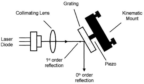
4-1 The Sanyo DL3149-056 laser diode ... 52

4-2 Schematic of an extended-cavity diode laser ... 54

4-4 Fabry-Perot interference fringes for three different mirror reflectivities. 59

4-5 Fabry-Perot cavity in a confocal arrangement. ... 61

4-6 Side-locking to a voltage signal. ... .. 63

4-7 Peak-locking to a voltage signal. ... .. 64

4-8 Schematic of the dual-laser setup ... 66

4-9 Photographs of the ECDL baseplate and housing ... 67

4-10 Photographs of the collimation process ... 69

4-11 Characteristic Power-Current curve for the Sanyo DL3149-056 laser diode ... 70

4-12 Photograph of a laser stabilized to a Doppler-broadened Iodine line.. 71

4-13 Pictures and schematic of a saturated-absorption setup ... 72

4-14 Schematic of a laser system locked to an iodine-stabilized Fabry-Perot cavity. ... 74

4-15 Frequency drifts of a laser side-locked to an Iodine transition .... 75

4-16 Frequency drifts of a laser peak-locked to an Iodine transition .... 76

5-1 Optical layout for the monolithic laser. ... 81

5-2 Photograph of the filter cavity . . . ... 83

5-3 Photograph of the monolaser baseplate ... 85

5-4 Photograph of the completed monolaser. ... 86

5-5 Transmission through and reflection from a well-aligned filter cavity. . 88

5-6 Filter cavity transmission spectrum with optical feedback. ...

89

5-7 Schematic of an AOM in a double-pass configuration ... 90

5-8 Monolaser frequency stability over a 5 minute period ... 91

5-9 Blue monolaser frequency stability over a 5 minute period when locked to the ion fluorescence signal. ... 92

6-1 Schematic of the ion trap setup ... 96

6-2 Depletion in an ion cloud. ... 97

6-3 Depletion in an ion crystal ... 98

6-5 Discrete quantum jump levels ... 100 6-6 Frequency dependence of ion fluorescence in the high red power limit. 102 6-7 Frequency dependence of ion fluorescence in the low red power limit. 103

Chapter 1

Introduction

1.1

Background

Atomic ion traps exemplify an experimental elegance that is difficult to surpass. They

permit physicists to study and control ions with exceptional precision to gain insight

into the quantum world. Ion traps come in many flavors and sizes [1, 2], and have been used to perform various experiments in a wide range of subfields.

This thesis is concerned with trapping 88Sr+ in a linear Paul ion trap. Owing to the electronic level structure of strontium, blue and infrared (IR) lasers are required

to trap, cool, and image the ion. Unfortunately, after the trapping has succeeded,

there is little further science that can be performed with these two lasers alone.

We can now ask what types of experiments become accessible if we introduce a third laser to address the 674nm red transition in 88Sr+. One can group the

possi-ble experiments roughly into three classes: quantum phenomena, ion probing, and

quantum information. Experiments in the first category, such as depletion, quantum

jumps, and the quantum Zeno effect, are able to test and verify the fundamentals of

quantum theory. The second type of experiments, such as temperature measurements and sideband cooling, use the red laser as a probe to determine and affect properties of the ions and ion trap system. The third class of experiments investigates how information can be stored and manipulated using trapped ions. This thesis will focus on the depletion, quantum jump, and temperature measurement experiments.

1.2

Overview

Before presenting the experiments in detail, a suitable background must first be es-tablished. Chapter 2 presents a broad overview of the ion trapping process. Sections

2.1-2.3 detail the geometry and mathematics pertaining to the trap used in our

stron-tium experiments. Section 2.4 describes the finer points of trap operation, including construction of the vacuum system, producing and detecting ions, and correcting for

any stray fields in the trap.

Chapter 3 presents the structure of the strontium ion and the theory behind

depletion, quantum jumps, and temperature measurements. In this chapter, one

can find calculations and predictions showing the data we expect to see when the

experiments are run.

Chapter 4 describes a first attempt at building a laser with sufficient frequency stability to observe the desired effects. Section 4.1 provides a theoretical background

of the important optical components used in constructing the setup. Section 4.2

presents the design for a dual-laser system, and Section 4.3 describes its construction.

Stability results are presented in Section 4.4.

Chapter 5 details the design and construction of a more stable laser than the

one described in Chapter 4. The important differences and expected performance improvements are highlighted throughout the chapter. Section 5.3 gives the stability measurements of this new red laser.

Chapter 6 presents experimental results. Using the laser constructed in Chapter

5, we show our depletion, quantum jump, and temperature measurement data.

Ad-ditionally, we describe the setup of each experiment and compare the results to the

theoretical predictions made in Chapter 3.

1.3 Contributions to this work

This work was performed in Prof. Isaac Chuang's laboratory at the MIT Center for Bits and Atoms. This project is part of an ongoing, long-term effort to realize

large-scale quantum computation in ion traps.

Robert Clark, Jaroslaw Labaziewicz, and Kenneth Brown all assisted me in con-structing the laser system introduced in Chapter 4. Several of the electronic

compo-nents necessary to operate the laser were built by Clark, and Labaziewicz designed

the software and hardware used for stabilizing the laser via electronic feedback. I fab-ricated the electronic feedback circuits designed by Labaziewicz, built and stabilized two external cavity diode lasers, and set up various locking and optical breadboard schemes. For each setup, I measured the stability to determine if it would be sufficient for our experiments (see Sec. 4.4).

The design and construction of the monolithic laser described in Chapter 5 was spearheaded by Labaziewicz. The idea was inspired by a setup employed by Prof. Kazuhiro Hayasaka of the Kansai Advanced Research Center in Japan. Labaziewicz and Chuang developed software to interface with an FPGA chip and lock the laser.

I aided in the monolaser construction and testing process by building the ECDL and

optics and performing some simple debugging.

The linear Paul trap used in these experiments was designed and fabricated in

Japan by Prof. Shinji Urabe's group at Osaka University. Brown designed much of

the vacuum chamber mounting system, and Labaziewicz was primarily responsible

for cleaning and installing the trap.

While Labaziewicz was refining the monolaser design, Clark taught me the ion trapping process. From then on, Brown and I typically worked together to trap ions for experimentation. Using the monolaser, Brown, Labaziewicz, and I were able to

Chapter 2

Ion Trapping

Ion traps have proven themselves to be an important tool for research in experimen-tal atomic physics. Since their development, ion traps have allowed researchers to make very precise spectroscopic measurements [3, 4, 5], perform fundamental tests of quantum theory [6, 7, 8], and determine the masses of various atoms and molecules to very high accuracy [9, 10]. Additionally, several groups have demonstrated quantum information processing and have implemented quantum algorithms on small numbers of ions [11, 12], providing a promising avenue for large-scale quantum computation.

There exist several different mechanisms for trapping ions. In general, charged particles may be trapped by electric and magnetic fields. However, as was first shown by Samuel Earnshaw [13], static electric or magnetic fields alone cannot provide con-finement in three dimensional space. This arises directly from Laplace's equation,

V2V = 0. For any local minimum, the potential in the surrounding region would be harmonic for small displacements: V = ax2 + by2 + cz2. Taking V2(ax2 + by2+ cz2)

gives a + b -t c = 0, implying that the potential cannot be simultaneously attractive

(or repulsive) in all 3 directions.

In 1936, Penning proposed a way to circumvent this restriction by designing a trap with superposed electric and magnetic fields [14]. Two decades later, Wolfgang Paul presented an alternative approach involving oscillating electric potentials to confine the ions [15, 16, 17]. Since the work in this thesis was performed exclusively in a Paul

2.1 The Linear Quadrupole Paul Trap

Paul traps use radio-frequency (rf) fields to create a quadrupolar trapping potential.

In his original paper, Paul presented a geometry involving a ring and two endcaps to

generate a stable trapping point at the center of the ring. Since Paul's initial design,

various new geometries for trapping ions with rf fields have been suggested, including the linear quadrupole trap [18, 19]. This design is comprised of four rods; two provide the rf voltage, while the other two are grounded (see Fig. 2.1). Segments on the ends of the rods may be biased to provide axial confinement. As opposed to the original

Paul traps that contained only one stable point, linear Paul traps provide a line of

stable points along the central axis, permitting a chain of ions to be trapped and

cooled.

5

K

Figure 2-1: Schematic of the linear Paul trap. Left: end view of the trap. Two

opposing rods carry a potential V = Uo + V0 cos(QTt), where V is the zero to peak amplitude of the rf voltage and U0 is a DC bias. The other pair of rods are held

at ground. Note also the coordinate system: and y point radially, while z points axially. Right: three-dimensional view of the trap. The outer segments of the rods (endcaps) are held at positive DC voltage.

To generate a purely quadrupolar field along the central trap axis, it is necessary for the four rods to be shaped like hyperbolas. Fortunately, calculation shows that alternate geometries, such as round or knife-edged rods, can produce quadrupolar fields to very good approximation [20]. As a result, most modern traps use these

constructions due to ease of fabrication and lower costs.

The positive, static voltage applied to the endcaps prevents the ions from leaking

direction only. The most general quadrupolar potential can be written:

bx,

Substitution into Laplace's equation gives:

V2[A(AX2

+ y2)] =

0

A+a = 0

As we expect, if the potential is attractive along x, it is repulsive along 9 (and vice versa). The potential forms a saddle point along the center of the x - y plane. Clearly, ions will escape along the 9 direction after a short time. However, as we will see, the ions can be confined if we rotate the potential at some frequency QT. Including the

possibility of a DC bias U, we may write the radial potential as:

· W,,(t) = 2 (UO+ Vo cos(QTt)) 1 + 2

2~~~

x02-

(2.4)

where V is the zero-to-peak amplitude of the rf potential and ro is the distance from

the center of the trap to the rods. This potential is plotted in Fig. 2.2.

Potential at t=O o · 0.5 0 a. 0 0 Q. 'ii a Potential at t=T12 0.5 0 0. -0.5 -0.5 y mm] x[mm U .. 0 0.5 [mm] -0.5 [MM]

~~x

Figure 2-2: The radial potential at two points in time, with UO = 0. Left: at t = 0,

the potential is attractive in : and repulsive in Y. Right: after half a period, the

situation has reversed, and the potential is now attractive in Y.

Armed with this potential, we can now examine the behavior of ions in the linear quadrupole trap. WVe will first solve the complete problem of a charged particle moving in this potential, from which we can calculate the stability criteria for the trap. We will then make some approximations which allow us to gain intuition about ion motion.

2.2 Full Solution: The Mathieu Equation

Given our expression for the potential (Eq. 2.4), we may calculate the equation of motion for an ion. Since there are no cross terms (e.g. xy) in the potential, the motion in x and y can be solved independently. Due to the symmetry in the setup (A -v), solutions for x and y should have the same magnitude, but with opposite signs. If we solve the system in the x direction for an ion with mass m and charge Q,

F = m= -QVDx (t)

(2.5)

where

·

(t)

= (UO

+ Vocos(QTt)) 1 +

(2.6)

Taking the gradient,

m+Q

(o±Vo

os(QTt)

=

0

(2.7)

d2x QU0 QVocos(QTt) = 0 (2.8)

+ k~r~

_r2±

dt2 mr0 mro

At this point, we can change variables to make the equation dimensionless. Let us make the following definitions (the reasoning will soon become clear):

QTt 4QUo 2QVo (2.9)

If we were to repeat this process along along the y direction, we would find that ax = -ay and q = -qy. Substituting the scaled x variables into Eq. 2.8 gives:

d2x 4 QUo QVO co(2) = 0 (2.10)

d

Q

d + (ax - 2q cos(2())x = (2.11)

do2

Eq. 2.11 is the exact canonical form of the Mathieu equation [21], whose solutions are well known. Since the physical goal is to trap ions, we seek stable solutions to the equation of motion (i.e. solutions bounded for all t). As demonstrated by Floquet

[22], a complete solution to the Mathieu equation can be written:

x(() = Ae"'q$(~)

+ Be-'q(-~)

(2.12)

where A and B are constants of integration, is a complex constant, and q is a function with period r [23]. Since X is periodic, we can expand Eq. 2.12 using

Fourier's theorem:

00 00

x(()

=

Ae/

>

2ne

n=-oo n=-oo

where the C 2n's represent the amplitude of each term in the Fourier series. With the periodicity of the solution now explicit, we can turn our attention to the e and e-" factors that appear in Eq. 2.13. Since is complex, it may be rewritten p = a + i. We notice immediately that if it has any real component (a 0), the trajectory is unstable since e or e-< goes to infinity as increases. Imposing this condition, the solution becomes:

00 00

x(() = A

E

C2ne

+ B

E

C2n

o

(2.14)

Applying Euler's formula (eiO= cos 6 + i sin 6),

00 00

x() =

A'

E

C2n

+ B'

+ /3)]

n=-o00 nL=-o0

with A' = (A+B) and B' = i(A-B). Given Eq. 2.15, the value of 3 alone determines the stability of a trajectory [24]. If is an integer, the solutions - called Mathieu functions of integral order - will be periodic but unstable. If

/3

We can now substitute the solution Eq. 2.15 into the original Mathieu differential

equation (2.11) and solve for values of a. and q that provide stable ion trajectories. This process is detailed thoroughly by N. McLachlan [25]. From these calculations, one can divide the a - q plane into regions of stability and instability. For certain values (q,a), the trajectory in the x direction will be periodic and bounded. If we

then repeat the process along and combine the results, we will find regions in a - q space where the ions are confined in both directions simultaneously (see Fig. 2.3).

Mathieu Stability Regions Mathieu Stability Regions 1 -0 -1 co S q q

Figure 2-3: Mathieu stability regions in the a - q plane. Left: Stability region along the x-direction (light grey). Right: Stability region along x or y only (light grey), and in both dimensions (dark grey).

Ions will be effectively trapped if (q,a) lies within the dark grey diamond in Fig. 2.3 (right). Recalling the definitions presented in Eq. 2.9, we can now determine the

values of

U

constants or geometrical measurements). Consider, as was typically done in this thesis, the case of no DC bias on the rf rods (U0 = 0). Calculation shows that the

maximum stable q value is .908 [25]. Recalling the definition of q, we find

2QVo < .908 (2.16)

mrQ

-Assunming a 88Sr+ ion in a trap with ro = .6mm,

Vo

<

V s2 (2.17)

From Eq. 2.17, we find a relation between V0 and QT that determines the stability of

the trap. Typical trapping values used in this thesis were V = 320 V and QT/27r =

17.5 MHz, giving a stable q of .16.

We have now solved the problem of trapping ions using only electric fields. By appropriately choosing the free parameters U, V0, and QT (and hence a and q), one

can determine whether or not the arrangement will be stable. Unfortunately, Eq.

2.15 is somewhat complex, making it difficult to gain intuition about ion behavior in the trap. By applying some approximations to the system, however, we may develop

insight into ion dynamics.

2.3 The Secular Approximation

Let us begin by qualitatively understanding the interaction between a trapped ion

and the surrounding electric fields. By construction, there is a trapping potential

oscillating at QT. This oscillation can send ions into forced vibration with drive

fre-quency QT and some small amplitude. At slower time scales, the ions effectively "see"

a harmonic potential in all directions. Analogously to classical simple harmonic oscil-lators, we expect the ion to undergo harmonic motion at some secular frequency WSec.

The total motion is given by the sum of the fast, driven motion (called micromotion) at frequency QT and the slow, secular motion at frequency wsec.

As before, with no bias on the rf rods, we begin by writing the equations of motion for x and y:

[ ]

r2

cos(Tt)

[

]

(2.18)

We qualitatively saw that the total ion motion was comprised of secular motion and micromotion. If we let x = xsec + x, and y = Ysec + Y,,

Xsec

1

O

t)

COS(QTt) (2.19)

Ysec + p mro Ysec + Yp

At this point, we introduce the secular (or pseudopotential) approximation [26, 27].

In this approximation, the amplitude of the micromotion is taken to be small as

compared with the amplitude of the secular motion (i.e. x, < Xsec). Additionally, since we expect the drive frequency QT to be larger than the secular frequency w,ec, we assume that , >> X ,ec Identical expressions hold for y. Substituting back into Eq. 2.19,

=

cos(Qt)

[

[Ysec

Solving the equation for the micromotion is now straightforward:

[ ]

=

[

(2.21)

y.

=mroT

As we may expect, the trajectory due to micromotion oscillates at the rf frequency

QT. Additionally, the amplitude is guaranteed to be smaller than the secular motion amplitude since we can rewrite the prefactor QVo/mr2Q2 as q/2, where q is a Mathieu paran-eter. For a stable trap, q cannot exceed .908, so

x,

expressions for the micromotion (Eqs. 2.20 and 2.21) into Eq. 2.19,

sec 202 Cos2(Qt) Xsec (2.22)

Ysec .." 0 T Ysec

If we again use the approximation that QT is fast compared with Wsec, we can time average Eq. 2.22 over one period of rf drive. Using that (cos2(QTt)) = 1/2,

Es1ec

V02

[

1

Jsec

2mr(

rT

The solutions to these simple differential equation are given by

xsec = A cos(wxt + ) (2.24)

Ysec = B cos(wyt + )

(2.25)

where

wx = Wy = v/Q T (2.26)

are the secular frequencies in the x and y directions. A schematic of an ion's position as a function of time is plotted in Fig. 2.4.

One particularly nice feature of the pseudopotential model is that it allows ap-proximation of the trap depth. We define trap depth as the maximum energy an ion can have before running into the rods [27]. The trap depth is calculated by treating the system classically and equating forces:

1 22

QD = 2mwrO

(2.27)

where Dx is the depth in the x direction. Rearranging and substituting for wx gives

QVc2

D,

Secular and Micro- Motions o0 0 0 D So o -o. o 2 3 4 5 6 7 '-'8 6 9 Time [)'lec_]

Figure 2-4: Secular motion and micromotion for a trapped ion. The large-amplitude, low frequency curve (blue) is the secular motion, while the high frequency red curve is the total ion motion. For this figure, QT = 5w and Ix, = .31xsecl.

If we again substitute typical experimental values (V0 = 320 V, QT/27r = 17.5 MHz,

ro = .6 mm), we find a trap depth of 6.4 eV. Given that we have been able to hold ions experimentally as low as 2 eV, these trapping parameters provide good confinement. Additionally, as we have seen earlier, they are well within the Mathieu stability region.

2.4 Operating the Trap

In addition to setting an appropriate rf drive frequency and voltage, several other factors must be addressed before we can trap ions. First, we need to ensure that the trap is in an ultra-high vacuum (UHV) environment. At high pressures, random collisions between the ions and background gas will impede the trapping process. Once the trap is under UHV, we need to devise a way of ionizing neutral strontium. Next, we need a way to image the ions. Finally, we should have the flexibility to compensate for any microscopic defects or stray fields in the trap that may alter the

2.4.1 Vacuum System

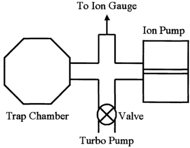
The UHV system in this experiment was built to achieve a vacuum of 10-10 torr. The design is relatively straightforward (see Fig. 2.5). The ion trap chamber (Kimball Spherical Octagon, MCF450-SS20400-A) connects to the vacuum system via a 2 3/4" conflat (cf) fitting. This fitting connects to three branches. The first branch connects to a valve, permitting attachment of a rough or turbo pump. This allows us to bring

the trap pressure from atmosphere down to

10

torr. The second branch connects

to an ion pump (Varian StarCell VacIon Plus 40). With a pumping speed of 20 L/s,

the ion pump can be used to evacuate the ion trap chamber to - 10

_{torr. The}

third branch connects to an ion gauge (Varian SenTorr) to monitor the pressure.

To Ion Gauge

Turbo Pump

Figure 2-5: Schematic of the ion trap chamber and vacuum assembly. See text for

details.

Before using the trap, it is "baked" by maintaining it at a temperature of 150°C for one week. The entire trap assembly is wrapped in aluminum foil, covered with heater tape, and wrapped with a second layer of foil. During this process, water vapor and hydrogen gas are driven off the interior surfaces and readily collected by the ion pump. Once an acceptable pressure has been reached, the heater tape and foil may be removed, and the system can cool to room temperature.

2.4.2 Ionization

In order to create ions from a neutral strontium source, an electron beam was fired at a strontium oven. The oven consists of a small piece of strontium wrapped in tantalum foil. A high current (typically 4.5 A) is passed through the foil, thereby

heating the strontium within and spraying neutral atoms towards the trapping site.

On the opposing side of the trap chamber sits a small coil of tungsten wire biased at -20 V. When a voltage is passed through the wire (typically 2 V), it emits a stream of

electrons which ionize the strontium in the trapping region. In practice, this method

is almost always effective for loading an ion cloud into the trap. A diagram of the setup can be seen in Fig. 2.6.

Figure 2-6: Picture of the trap chamber showing the strontium oven and electron

gun. Collisions between the electrons and neutral strontium causes ionization at the

trapping site.

2.4.3 Ion Detection

When strontium ions are irradiated with the proper frequency of laser light, they will

absorb photons and transition to higher energy states. Soon thereafter, the atoms

Flu(

--- 50:50 Beam

Splitter

'

Achromatic

/ Doublet Lenses

Figure 2-7: Optical setup for detecting and imaging ions. The ion fluorescence signal is focussed by a 100mm meniscus lens and a pair of achromatic doublet lenses (100mm and 500mm focal lengths), providing r-7X magnification. A 50:50 beam splitter sends

half the signal through a pinhole and into a photomultiplier tube (PMT), while the

other half is sent to a CCD camera for imaging.

different methods to detect this fluorescence. The first is a simple photon-counter setup. Light emitted from the ion trap is focussed through a pinhole to reduce

scatter, then sent to a photomultiplier tube (PMT). The output signal from the

PMT is directed to a lab-built FPGA controller for signal processing. This allows us to count the total number of photons received during a user-specified period of integration. Additionally, the controller can sync to an external trigger so that any periodicities in the ion fluorescence signal may be observed. A schematic of the setup

is shown in Fig. 2.7.

(Princeton Instruments PhotonMax). The camera contains a silicon charge-coupled

device (CCD) segmented into a grid of 512 x 512 light-sensitive cells. The total number of photons per frame incident on each cell is recorded, and the result is output to form an image. Software designed in lab allows us to set the integration time (lOOms minimum), measure the total fluorescence intensity, digitally zoom in on regions of interest, and perform background subtraction. Images of trapped ions can be seen in Fig. 2.8.

Trapped Ion Cloud Trapped Ion Chain

Figure 2-8: CCD camera image of trapped ions. Left: a large, hot cloud of trapped ions. Right: three individual ions lined up along the trap axis.

2.4.4 Compensation

When performing ion trap experiments, it is necessary for the ions to sit exactly along the nodal line of the rf drive. Unfortunately, trap defects and stray electric fields make this condition difficult to realize. A direct consequence of such imperfections is an increase in micromotion amplitude, which may obscure delicate spectroscopic features and cause Doppler shifts in atomic transition frequencies [28]. We therefore need to

detect and eliminate micromotion.

The best way to minimize micromotion is to push the ions back to the rf null. To accomplish this, compensation electrodes with static DC biases are built into the ion trap. By including two radial biases and one axial bias, it is possible in theory to perfectly compensate the trap along all three degrees of freedom.

Both the PMT and the camera can be used to detect micromotion (see Fig. 2.9). Recalling Eq. 2.21, we expect the micromotion oscillation to occur at the rf drive frequency QT. Thus by triggering the photon counter at the drive frequency, we can

observe periodicities in the ion fluorescence due to micromotion. Similarly, micro-motion causes an ion image to become spread out when viewed with a camera. By

appropriate adjustment of compensation voltages, the oscillations on the PMT and

spreading on the camera will vanish, and the ions will sit along the rf node.

Z-axis Compensation V 9 a, U C tu 1; . x X 0.05 0.1 0.15 0.2 -100 -50 0 50 100

time psl radial distance [pm]

Figure 2-9: Detection of Ion Micromotion. Left: micromotion oscillations for endcap voltages of 7V (blue), 31V (green), and 45V (red). The green curve exhibits good compensation, while the blue and red curves show a relative phase flip. Right: CCD camera image of a single ion with a large radial micromotion.

2.5 Summary

In this chapter, we have discussed the theory and experimental considerations of

trapping ions. Starting with a relatively simple potential, we were able to solve the equations of motion and derive stability criteria for ions in a linear Paul trap. We were also able to gain insight into ion behavior and calculate the trap depth by making some small approximations. Finally, we have discussed the construction and operation of ion traps. At this point, we are ready to consider the interesting physics that confined strontium ions can offer.

Chapter 3

The Strontium Ion

This chapter will characterize the strontium ion and describe some experiments that may be performed when ions are trapped. Although there exist many suitable atomic species for ion trapping, atoms in Group II of the periodic table are preferable. After ionization, these atoms will contain a single valence electron, and their electronic level structure is vastly simplified.

Research groups around the world work with various atoms, including 9_{Be+ [29],}

4 0_{Ca+ [30, 31], 88Sr+ [32, 33, 34], and 'lCd+ [35]. We have chosen to trap 88Sr+ since}

all of its relevant transitions can be addressed with diode lasers, giving a compact

and relatively inexpensive setup. We shall now turn our attention to the strontium

energy level diagram and discuss the three important transitions.

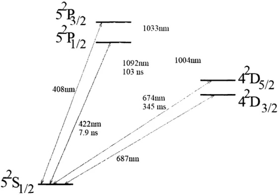
3.1

Energy Level Structure

A partial energy level diagram for strontium is shown in Fig. 3.1. A variety of states are displayed along with their transition wavelengths and lifetimes. For our exper-iments, there are three important transitions: 52S1/2 -4 52P1/2 (422nm), 52P1/2

--42D3/2 (1092nm), and 52S1/2

--

' 103rlull

/2 J o

674

..

4i5/2

1A5 ,he -" +

ILJ /,

/i

S.

p

"

1/2

Figure 3-1: Energy level diagram for 88Sr+. The relevant transitions are at 422nm (blue), 674nm (red), and 1092nm (IR).

3.1.1 The 422nm Transition

Before carrying out any experiments, the atoms must first be detected and cooled. The 422nm blue transition is used to accomplish both. When 422nm light impinges on a trapped strontium ion, it induces the transition 52S1/2 -- 52P1/.2 On average,

the atom will decay back to the ground state after 7.9ns, emitting a 422nm photon. This photon can then be detected with a photon counter or CCD camera (see Sec. 2.4.3).

The absorption and emission of the blue photon can also reduce the energy of the atom through the Doppler cooling process [36, 37]. Suppose the frequency of the laser is tuned slightly lower than the transition frequency. Atoms moving towards the beam will effectively "see" a higher frequency due to the Doppler effect. As a result, the atom will be on resonance, absorb the photon, and receive a momentum

.·'

..

.

.

kick of

hk

lose hk units of momentum each time a photon is scattered. In this way, the motion

and temperature of the ions can be reduced.

Unfortunately, there is a limit to the temperatures achievable by Doppler cooling [38]. Though photon emission on average imparts no momentum to the atom, each individual event causes a small recoil. Thus, there is a small amount of heating associated with emission, creating a Doppler cooling limit of kBT = hF/2, where kB

is Boltzmann's constant and F is the natural linewidth of the transition. For the

422nm strontium line, calculation of the Doppler limit yields T=76 1K.

Experimentally, however, the ion temperature was determined to be 660 mK -several orders of magnitude hotter than the Doppler limit (see Fig. 3.2). Two factors

Crystallization y31.8182 a =18.7297 1 1UUU 10000

9000

Figure 3-2: Laser-induced fluorescence at 422nm from a cold chain of ions. As the fre-quency is increased towards resonance, the fluorescence increases. Above resonance, however, laser heating decrystallizes the chain and the signal drops. The lineshape is a convolution of a Lorentzian (natural linewidth) and a Gaussian (Doppler broadening).

contribute to this value. First, the blue laser was simultaneously being used to cool

the ions and determine their temperature. This results in an upper temperature

bound, not an accurate measurement of the true temperature. Second, only one degree of freedom was being cooled. To reach the Doppler limit, all three directions must be addressed concurrently. At this point, it is difficult to tell whether or not this temperature is sufficient to observe the red laser effects since the measurement provides only an upper bound. However, as we shall soon see, the red laser itself can

be used to more accurately determine ion temperature.

3.1.2 The 1092nm Transition

A strontium ion in the 5

P1/

state will decay to the 4

D

/

metastable state with

probability 1/14. After a short amount of time, all of the strontium ions would be shelved in the D3/2 state, and the detection and cooling processes would fail. As a

result, we employ a 1092nm laser to repump the ion back to the P1/2 state. This

prevents depopulation of the ground state and allows us to continue running our

experiments as usual.

3.1.3 The 674nm Transition

The 674nm line in 8 8Sr+ is a strongly forbidden electric quadrupole transition. Its frequency has been reported as 444 779 044 095 484.52±.10 Hz [39], and represents one of the most accurately measured quantities in all of atomic physics. Since the transition is strongly forbidden, its lifetime is large (345ms) and its natural linewidth is small (0.4 Hz). The crux of this thesis revolves around addressing this narrow line in order to probe trapped strontium ions. In particular, we wish to observe the effects

of depletion and quantum jumps and accurately measure the ion temperature.

Before describing these effects in greater detail, it is useful to mention some of the other applications of the 674nm line. Recently, there has been interest in using trapped ions for optical clocks [40]. Since visible radiation is of higher frequency than the microwave radiation used for cesium atomic clocks, optical clocks will have greater

time resolution and should prove to be more accurate. P. Gill et. al. have

demon-strated a frequency standard based on the 674nm line that is three times more stable

than the current cesium standard at NIST [41]. Additionally, the 5

_S1/

2

-- 42D5/2

transition has been proposed as an optical qubit for ion trap quantum computation [42, 43]. In these schemes, the S1/2 state serves as the logical 10), the D5/2 state is the

logical 1), and the 674nm radiation is used to couple the two states to each other.

3.2 Linewidth Considerations

The natural linewidth of the 674nm transition is 0.4 Hz. Experimentally, however, the linewidth appears much broader. There are two significant effects: Doppler broaden-ing and power broadenbroaden-ing. Doppler broadenbroaden-ing is the dominant process; even if we

were to cool to the Doppler limit, the resultant linewidth is calculated to be 125 kHz

(a full derivation of the Doppler linewidth will be given in Sec. 4.1.3). Therefore, the

narrow Lorentzian natural linewidth will be heavily shrouded by the broad, Gaussian

Doppler profile.

If we were to employ techniques to cool below the Doppler limit, narrower linewidths could be attained. However, as the linewidth continues to shrink, one will begin to observe power broadening effects. When intense laser light irradiates an atom, it will be possible for slightly off-resonant frequencies to induce the transition [44]. This

off-resonant excitation makes the absorption line appear broader than its natural

linewidth. For a transition with a natural linewidth ry, the steady state solution to

the Optical Bloch Equations allows calculation of the power-broadened linewidth -y'

[45]:

y'= vty+

S

(3.1)

In Eq. 3.1, so defines the on-resonance saturation parameter,

21aQ2 I

where Q is the Rabi frequency, I is the laser intensity, and I, is the saturation intensity of the transition, given by

7rhc

IS-= 3A3 _-(3.3)

Plugging in numbers for the 674nm transition, we find that I = 1.9 x 10-6 W/m2. Thus, for a typical 200 LW beam focussed to a 200 um spot size, we calculate a saturation parameter so 1 x 109 and a power-broadened linewidth of y' 10 kHz.

3.3 Depletion, Quantum Jumps, and Temperature

Measurements

We shall now turn our attention to three of the interesting experiments that can be

performed with trapped strontium ions using the 674nm transition.

3.3.1 Depletion

Consider the strontium level structure as shown in Fig. 3.1. If we irradiate the atom

with only 422nm and 1092nm radiation, it will cycle primarily between the S and P

states, occasionally decaying to the D3/

state and consequently repumped by the IR

laser. Since the atom emits a 422nm photon each time it decays from the P state to

the S state (on average, every 7.9ns), the atom will fluoresce quite strongly and can

be easily observed.

Now consider the effects of shining all three lasers at the atom simultaneously. If the red laser is significantly more powerful than the blue, an atom in the ground state will begin to cycle between the S state and the D5/2 state. This causes a depopulation

of the S -

P transition, and the 422nm photon emission rate will decrease. As a

result, part of the fluorescence signal will disappear, since the imaging optics cannot detect an ion in the D state. This phenomenon is termed depletion, and should be visible in both clouds and crystals. Given a moderately stable and powerful red laser tuned to the transition frequency, depletion should be easily observable.

3.3.2 Quantum Jumps

Quantum jumps [46, 47, 48] are fascinating physical phenomena closely related to depletion. Let us again consider a strontium ion in the ground state. If we were to look for depletion, we would tune the red laser to the transition frequency, increase the red power as much as possible, and observe a dip in the fluorescence signal for the entire time the red laser was on. A simple question can now be asked: what happens

when the red laser power is decreased?

In this case, the simple explanation is the correct one. We have an atom in the

S state, a blue laser trying to excite it the P state, and a red laser pushing it to the

D5/2 state. Since there can only be one transition at a time, it is easy to imagine a

competition between the blue and red lasers. For some value of relative laser powers,

the atom will have some probability p of transitioning to the D5/

state, and some

probability 1 - p of being excited to the P state. If the red laser power is then

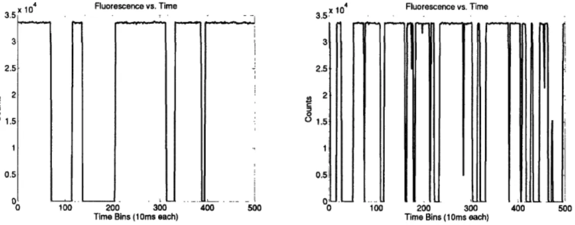
increased, so will the probability of transitioning to the D5/₂ state. If we increase the red laser power dramatically, p approaches 1, and we find ourselves in the depletion regime. Of course, if the red laser power is reduced dramatically, p approaches 0, and we see the usual fluorescence signal.

Naturally, the intermediate regime is the most interesting. Let's consider the

fluorescence signal of a single ion over time. When the atom cycles between the S and P states, 422nm photons will be continuously emitted, giving some number of counts per time window. Although there will always be some statistical noise in the number of counts, we expect the value to remain relatively steady. Every so often, however, the red laser will successfully excite the S - D5/2 transition. While the

atom remains in this state, no blue photons can be emitted. Therefore, we expect our fluorescence signal to drop to 0. The number of counts will increase to the previous value only after the atom has decayed from the D5/2 state and begins transitioning

between S and P once more.

These random hops in the fluorescence signal are the signature of quantum jumps. Every time the single ion finds itself in the ground state, it faces a probabilistic choice

to transition to either the P or D5/₂ state. Although we are able to predict the long-term fractions of time spent in each state, we can never with certainty predict the behavior in the short term. Recent work [49] has analyzed over 200,000 quantum jumps of a single strontium ion, demonstrating strongly randomized behavior of the system. For this reason, many researchers are interested in exploiting quantum jumps for random number generation.

An important theoretical problem is to determine the relative red and blue

intensi-ties necessary to observe quantum jump effects. Unfortunately, the analytical

expres-sions describing the system cannot be cast into an enlightening or easily interpretable form [50]. Consequently, we solved the problem numerically using Mathematica.

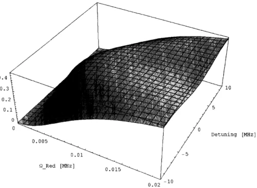
We wish to find the probability of being in the D5/₂ state as a function of red laser Rabi frequency (i.e. power) and detuning. Setting the blue laser on resonance with a Rabi frequency of 10 MHz, we determined this probability over a range of red Rabi frequencies and detunings (see Fig. 3.3).

//·7

-Figure 3-3: Numerical solution to the 3-level problem with spontaneous emission. The probability of being in the D state is plotted as a function of red Rabi frequency

We see that for

10 kHz, the probability of finding the atom in the D state

remains relatively uniform. This corresponds to the low end of the depletion limit,

where the red power is strong compared with the blue. Therefore, we would expect

the best quantum jump contrast to be found in the regime where 2 kHz <

10

kHz.

We also notice that the probability varies little over a detuning range of 20 MHz.

The calculated profile is directly related to the blue laser power. The blue Rabi

frequency of 10 MHz causes the S -+ D5/₂ transition to be broadened; as a result, the

red laser can be slightly detuned and still excite the transition. The small dip around

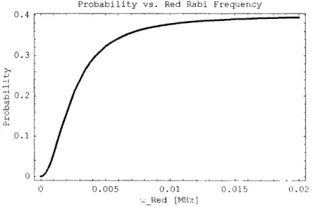
resonance is a manifestation of the Autler-Townes effect [51], which predicts a dip whose size is proportional to the strength of the blue laser. However, since we will only work with low to intermediate blue power, we will not expect to see any detuning effects. As a result, we can produce a simplified version of Fig. 3.3 by setting the detuning equal to 0 (see Fig. 3.4). This confirms that we should hunt for quantum jumps with a red Rabi frequency between 2 kHz and 10 kHz.

Probability vs. Red Rabi Frequency u.4 0.3 -r-52 0.2 rrJ LI 0.1 0 0 0.005 0. 01 C. 015 0.02 'x Red [MIlz3]

Figure 3-4: Probability of being in the D state as a function of Rabi frequency with the red laser on resonance.

To gain intuition about the dynamics of the system, I wrote a Mlonte-Carlo

blue laser R.abi frequencies as input, and outputs the simulated fluorescence signal over several seconds. Using the results of the previous analysis, I was immediately

able to identify a workable range of red Rabi frequencies in which to look for jumps. Fig. 3.5 shows the output of two different simulations with slightly different red Rabi frequencies.

3 104 Fluorescence vs. Time 3 1 Fluorescence vs. Time

3.5,3

_~~~~~~~~~~~~~~~~~~~~--

I

L

Time Bins (10ms each) Time Bins (10ms each)

Figure 3-5: Monte-Carlo simulation of quantum jumps for two different red Rabi

frequencies. Left:

MHz,

kHz. Right:

MHz,

kHz.

For the 5 seconds of simulated data, it is clear that there are many more quantum jumps at the higher red Rabi frequency (as expected). Re-running the simulation over a range of red Rabi frequencies, I found that quantum jumps were discernable from Qred=2 kHz to Qred=40 kHz. This is great news for our experiment, since we

will expect jumps to be observed for over 2 orders of magnitude in red power.

3.3.3 Temperature Measurements

As mentioned in Sec. 3.1.1, scanning the blue laser gives an inaccurate measurement of ion temperature. To improve the measurement, we will instead seek to scan the red laser. Since the red laser does not address the cooling S --, P transition, we can fix the blue laser at a single frequency (and therefore fixed cooling) while independently sweeping the red laser. This will allow us to find the Doppler linewidth of the ions, from which we can extract the temperature.

cl ---

I--L

F_

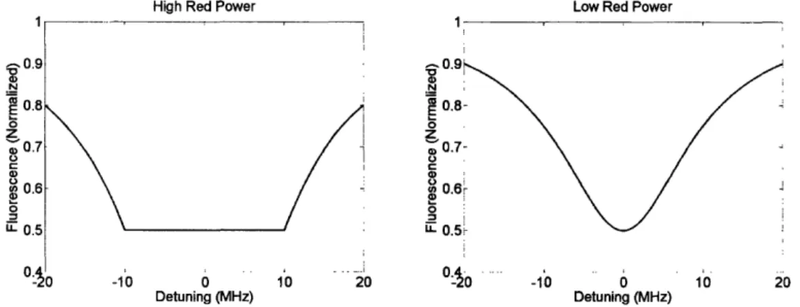
Let us consider the effects of sweeping the red laser across the 674nm transition. For red laser intensities at and above I, and low blue power, the probability of being in the D state on resonance is 1/2. Since the natural lineshape is Lorentzian, slightly off-resonant light will be able to excite the transition. However, we can never populate the D state more than 50% of the time. Therefore, for large red power, we can expect a profile that has Lorentzian tails, but flattens out across all frequencies which would give saturated excitation (see Fig. 3.6). By reducing the power, this phenomenon becomes unimportant, and we can observe the full line.

High Red Power Low Red Power

04O .. -10 0 10 20 Detuning (MHz) Detuning (MHz)

Figure 3-6: Expected spectrum of the 674nm line for high and low red laser power. Left: predicted fluorescence for high red power. Since the maximum population in the D state is only 1/2, we predict a flat bottom to a Lorentzian. Right: when the power is lowered and the amplitude of the Lorentzian is smaller, we avoid the saturation barrier and the full lineshape is recovered.

Notice, however, that the line would still be broadened to -20 MHz by the blue laser. To circumvent this effect, the blue laser intensity must be reduced below saturation. Unfortunately, as the blue power is decreased, it becomes more difficult to image, cool, and keep an ion crystal. In all likelihood, this will be the limiting factor in making temperature measurements. Our final upper bound will depend upon how low we can set the blue power and still run the experiment.

Resolved sidebands represent a more accurate method of extracting the ion tem-perature. In the limit of a single, cold ion, the red laser is able to excite the S - D5/2

transition when its detuning is an integer multiple of the secular frequency [52]. To

determine the temperature, we simply have to make a measurement of the peak

am-plitudes.

Let us think about the 674nm absorption spectrum of a trapped strontium ion.

Naturally, when the red laser is tuned to a frequency w

o resonant with the transition,

there will be strong absorption. However, this is not the only frequency at which we can observe a resonance. Since the atom is moving in a harmonic pseudopotential with some frequency w,,sec, the absorption and emission spectrum will have additional components at woinwsec, where n is an integer. For these sidebands to be observed, it

is imperative that the linewidth of the transition be smaller than the secular frequency.

Recall that though the natural linewidth of the 674nm transition is 0.4 Hz, Doppler broadening effects will yield a linewidth of order 100 kHz (when the ion is cooled to the Doppler limit). Given that the secular frequencies of our linear Paul trap are -1 MHz, we will be able to resolve sidebands provided our ions are cold enough.

The ratio of sideband amplitudes amplitudes can be used to determine the average

number of motional quanta, (m). As derived in Ref. [53], the ratio of the upper (w = Wo + UWsec) to lower (w = a - Wsec) sideband amplitudes is given by

Aupper (m)

+

When (m) is small, there will be a clear disparity in sideband amplitudes, and (m) can easily be determined via. Eqn. 3.4. Since the population (m) arises from a ther-mal distribution, we can use the standard Planck formula from statistical mechanics

to write [54]:

1

(m)= rh,

(3.5)

e kBT

-Rearranging for temperature, we find that

kBT

Therefore, simply by measuring the ratio of peak hights, one is immediately able to determine the average number of quanta (m) as well as the ion temperature. This represents a highly accurate method of measuring temperatures of only a few /zK

while leaving the system intact.

For Eq. 3.4 to give good results, we must be in the low (m) limit. If the number of motional quanta is large, then the upper and lower sidebands will have approximately

equal amplitudes. In this case, we must take the ratio of the sideband to carrier

amplitude:

or alternatively,

Aupper

112((m) +

)

(3.8)

where is the Lamb-Dicke parameter, given by

71 = kxo = A h (3.9)

A

Once r7 and the amplitude ratios are calculated, we again can immediately determine (m) as well as the ion temperature.

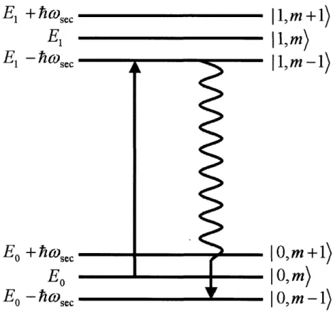
3.4 Sideband Cooling

Sideband cooling represents the next class of ion trap experiments. Although sideband cooling is slightly beyond the scope of this thesis, it deserves a few words on account

of its great importance.

Sideband cooling [55, 56, 57] exploits the physics of resolved sidebands to cool ions below the Doppler limit to their motional ground state. This process eliminates

E

+ Csec

E -AWsec

E

+

Cosec

Eo

E

o

-Arsec

Il,m+l)

Il1,m)

1,m-1)

IO,m+1)

IO,m)

IO,m-1)

Figure 3-7: Energy level diagram for sideband cooling. 0 and 1 correspond to the

S and D5/

states (respectively), and m is the number of motional quanta. After

exciting an atom in the state 10, m) with radiation of energy E

- Eo - hw, the

atom will on average decay to the state 10, m - 1), losing one motional quanta in the process.

negative effects due ion motion (e.g. Doppler shifts, micromotion), and is a necessary

precursor to implementation of logic gates in ion trap quantum computation.

Consider the energy level diagram in Fig. 3.7. Suppose we have an atom in

the ground electronic state with some number of motional quanta m. To begin the

sideband cooling process, we irradiate the atom with laser light of frequency wO - Wsec,

where wo again is the on-resonance transition frequency. After excitation, we are now in the 1, m,- 1) state. The atom then spontaneously decays, landing in the 10, m),

0, mn - 1), or

10,