Walking Faster in a Triangulation

(1)

HAL Id: inria-00493046

https://hal.inria.fr/inria-00493046

Submitted on 17 Jun 2010

HAL is a multi-disciplinary open access

archive for the deposit and dissemination of

sci-entific research documents, whether they are

pub-lished or not. The documents may come from

teaching and research institutions in France or

abroad, or from public or private research centers.

L’archive ouverte pluridisciplinaire HAL, est

destinée au dépôt et à la diffusion de documents

scientifiques de niveau recherche, publiés ou non,

émanant des établissements d’enseignement et de

recherche français ou étrangers, des laboratoires

publics ou privés.

Walking Faster in a Triangulation

Pedro Machado Manhães de Castro, Olivier Devillers

To cite this version:

Pedro Machado Manhães de Castro, Olivier Devillers. Walking Faster in a Triangulation. [Research

Report] RR-7322, Inria. 2010, pp.15. �inria-00493046�

(2)

a p p o r t

d e r e c h e r c h e

ISSN 0249-6399 ISRN INRIA/RR--7322--FR+ENG

INSTITUT NATIONAL DE RECHERCHE EN INFORMATIQUE ET EN AUTOMATIQUE

Walking Faster in a Triangulation

Pedro Machado Manhães de Castro — Olivier Devillers

N° 7322

(3)

(4)

Centre de recherche INRIA Sophia Antipolis – Méditerranée 2004, route des Lucioles, BP 93, 06902 Sophia Antipolis Cedex

Téléphone : +33 4 92 38 77 77 — Télécopie : +33 4 92 38 77 65

Walking Faster in a Triangulation

Pedro Machado Manhães de Castro , Olivier Devillers

Thème : Algorithmique, calcul certifié et cryptographie Équipe-Projet Geometrica

Rapport de recherche n° 7322 — June 2010 — 15 pages

Abstract: Point location in a triangulation is one of the most studied prob-lems in computational geometry. For a single query, stochastic walk is a good practical strategy.

In this work, we propose two approaches improving the performance of the stochastic walk. The first improvement is based on a relaxation of the exactness of the predicate, whereas the second is based on termination guessing.

Key-words: Point location, Delaunay triangulation

(5)

Marcher Plus Vite Dans une Triangulation

Résumé : La localisation d’un point dans une triangulation est un des prob-lèmes les plus étudiés en géométrie algorithmique. Pour un petit nombre de requêtes, la marche stochastique est une bonne stratégie en pratique.

Dans ce travail, nous proposons deux idées qui améliorent les performances de la marche stochastique. La première est basée sur une relaxation de l’exactitude du prédicat d’orientation, tandis que la deuxième est basée sur une tentative de divination de la longueur de cette marche.

(6)

Walking Faster in a Triangulation 3

1 Introduction

Point location in triangulations is a classical problem in computational geom-etry [6]. Given a query-point q and a triangulation in Rd_{, the problem is to}

retrieve the simplex containing q.

In two dimensions, locating a point has been solved in theoretical optimal O(n) space and O(log n) worst-case query time a quarter of a century ago by Kirkpatrick’s hierarchy [8]. However, alternative methods using simpler data-structures, with good performance in practice, are still used by practitioners. Amongst these methods, walking from a simplex to another using the neigh-borhood relationships between simplices, is a simple method which does not need any additional data-structure [4]. Walking performs well for Delaunay tri-angulations of evenly distributed points [5], but has a non-optimal complexity. Building on the simplicity of the walk, the Jump & Walk [9] and the Delaunay hierarchy [3] improves the complexity while retaining the simplicity of the data-structure. The main idea of these two structures is to find a good starting point for the walk to reduce the number of visited simplices.

Walking and Delaunay hierarchy are both implemented in the Computa-tional Geometry Algorithms Library [2] (Cgal): Cgal 2D Triangulations [12] and Cgal 3D Triangulations [10]. This work aims to improve the implementa-tion of such locaimplementa-tion strategies in Cgal.

Our Results. We describe two modifications in the stochastic walk strategy of Devillers et al. [4] which improve performance. The first one proposes a filtering scheme called predicate relaxation. The second one avoids to compute unnecessary orientation tests through a termination guessing strategy.

2 Preliminaries

2.1 Stochastic Walk

Given a triangulation T of Rd_{, with n vertices and m simplices, a query-point q}

and a simplex σ ∈ T , the stochastic walk [4] is a strategy to locate the simplex of T containing q, from σ.

First, let us define the visibility graph of a triangulation T and a query point q. The visibility graph of T and q, is a directed graph (V, E), where V = {s1, s2, . . . , sm} is the set of simplices of T , and a pair of simplices (si, sj)

belongs to the set of arcs E if si and sj are neighbors in T and the supporting

plane of their common facet separates any point in the interior of si from q (in

other words, segments formed by a point inside siand q intersect the supporting

plane of the common facet of si and sj). We will denote the visibility graph

of T and q by VG(T , q), or simply VG when there is no ambiguity. When two simplices siand sj are such that (si, sj) ∈ VG, we will say that sj is a successor

of si.

Let us introduce three walks based on the graph VG: (i) A visibility walk consists in repeatedly walking from a simplex sito an adjacent simplex sj of si

such that (si, sj) ∈ VG. (ii) Given an initial point p ∈ σ, a line-walk consists of

a visibility walk such that each visited simplex intersects the segment pq. (iii)

(7)

4 P. de Castro & O. Devillers

A stochastic walk is a visibility walk where the next visited simplex, from a simplex s, is randomly chosen amongst the successors of s.

The three walks above start from σ and ends at the simplex containing q. It is proved that arbitrary visibility walk does not always end (even in R2_{). The line-walk takes O(m) time in the worst-case, though it is proved}

to take O(√n) for Delaunay triangulation of points evenly distributed in the unit square [1] and ˜O(√3_n)1 _{in the unit cube [9]. For non-Delaunay}

triangu-lation, the stochastic walk finishes with probability 1 [4], though it may visit an exponential quantity of simplices for arbitrary triangulations in the space (even in R2_{). In practice however, it answers points location queries faster than}

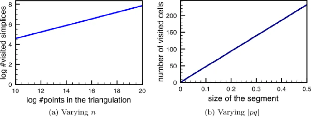
the line-walk [4]. Stochastic walk is the current choice of Cgal for the walking strategy [12, 10], in both dimensions 2 and 3. If the vertices of T are in general position and T is Delaunay, the stochastic walk visits at most O(m) simplices. Furthermore, if points are evenly distributed inside the unit cube it is conjec-tured that the stochastic walk visits an expected O(|pq| · n1/d_{) simplices (see}

Figure 1) where |pq| is the euclidean distance between a point p ∈ σ and q2_.

10 12 14 16 18 20

log #points in the triangulation

0 2 4 6 8 lo g # vi si te d si mp lice s (a) Varying n 0 0.1 0.2 0.3 0.4 0.5

size of the segment

0 50 100 150 200 n u mb e r o f vi si te d ce lls (b) Varying |pq|

Figure 1: Complexity Conjecture. (a) shows the average number of visited sim-plices by a stochastic walk done from the simplex containing the point (1/2, 1/2, 1/4), to the query-point (1/2, 1/2, 3/4), in several Delaunay triangulations of 210

, . . . , 220

points evenly distributed in the unit cube. (b) shows the average number of visited simplices by a stochastic walk done from the simplex containing the point (1/2, 1/2, 1/2−l/2), to the query-point (1/2, 1/2, 1/2+l/2), for l = 0.00, 0.01, . . . , 0.50, in several Delaunay triangulations of 220

points evenly distributed in the unit cube.

The primary ingredient of the stochastic walk is the orientation test. Given d+1 points p0(x0 0, . . . , x0d−1), . . . , pd(xd 0, . . . , xd d−1), we define the orientation

test as the sign of the following determinant: orient(p0, . . . , pd) = sign x0 0 . . . x0d−1 1 .. . ... ... ... xd 0 . . . xd d−1 1 ∈ {−1, 0, +1}. (1) 1

g = ˜O(f (n)) means that g = O(f (n) · h(n)), where h(n) is a polynomial of the logarithm

of n.

2

The |s| term in the big-O is an abuse of notation. Indeed, it is a ratio of two quantities having the same unity of measure. Here is the shortcut: |s| abbreviates |s|/δ (when it applies), where δ is the diameter of the domain boundary. As the domain is bounded (independently of n), then δ is a constant. And hence, we decide to just write |s|/δ = O (|s|).

(8)

Such expressions, which are the sign of a polynomial, are called predicates. The underlying polynomial, from which we will extract the sign for a given input, is called the predicate polynomial (here, the determinant of a matrix with d(d + 1) variables).

During the construction of T , every sequence of vertices of a simplex is (by convention) positively oriented. In other words, each simplex of T has d + 1 vertices v0, . . . , vd, placed on p0, . . . , pd respectively, and orient(p0, . . . , pd) =

+1.

Let q be the query point, and s be a simplex of T , with vertices on points p0, . . . , pd. Then, an adjacent simplex s′ is the successor of s iff the supporting

plane of their common facet (say the facet containing the points p1, . . . , pd)

separates p0and q, which is true iff orient(q, p1, . . . , pd) = −1.

Before describing the stochastic walk procedure, let us remind a well-known trick to handle queries which are not inside the convex hull of T . It consists into compactifying Rd _{into S}d _{by: (i) adding a point at infinity p}

∞, and then

(ii) gluing p∞ and each facet of the convex hull of T , forming new simplices

(one for each facet). These new simplices are called infinite simplices.

Now we will describe the fundamental procedure of the stochastic walk al-gorithm, which runs for each visited simplex. Assume s is the current simplex being visited, and i is a random index chosen from 0 . . . d.

Selecting next simplex to visit. The adjacent simplices sj of s, opposite

to the vertex v of sj, for j = 0 . . . d, are tested sequentially starting at si (i

random) to be a successor of s. The first simplex, which is a successor of s in the sequence, is selected.

Simplex found. When there is no more successors of s, then s contains q, and the remaining work is to count the number of orientation tests giving 0 as result so as to know exactly if q is inside s or on its boundary (and which piece of boundary).

Simplex not found. _{If s is infinite, then q is outside the convex hull of T .} We will consider here a well-known modification of the basic procedure above, consisting simply into not selecting the previous visited simplex as a candidate to be the next simplex to visit [4]. This effectively avoids one orien-tation compuorien-tation. To do this modification one needs only to remember the previous visited simplex during the walk and compare it with sj.

The above-mentioned approach leads to an expected cost which does not exceed (d + 1)/2 orientation tests per simplex visited during the walk. Suppose we run the procedure above on a simplex s and a query point q, then, as we skip the visited simplex, there are a total of d simplices to be tested. At the same time, in the worst case, s has only one successor 3

. And hence, as there is an equal 1/d probability that the i-th simplex tested is a successor of s, the expected number of orientation test computations is bounded by Pdi=1i/d = (d + 1)/2.

Now the total cost of the walk depends on the expectation of the number of visited simplices (which is unknown even for points evenly distributed in the unit square). See in Figure 2 the distribution of simplices computed experimentally for some particular cases in two and three dimensions.

3

s might have no successor at all, but this case will not influence the average number of orientation tests needed, since it occurs only once, at the end of the walk.

(9)

1100 1150 1200 1250

number of simplices visited during the walk

2^20 points evenly distributed in the unit square

Walk from (1/2, 1/4) to (1/2, 3/4) (a) Square 180 200 220 240 260 280

number of simplices visited during the walk

2^20 points evenly distributed in the unit cube

Walk from (1/2, 1/2, 1/4) to (1/2, 1/2, 3/4) (b) Cube 1800 1850 1900 1950 2000 2050 2100

number of cells visited during the walk

2^20 points evenly distributed on an ellipsoid centered at (1/2,1/2,1/2), axes size: x: 1/3 y: 2/3 z: 1 Walk from (1/2, 1/2, 1/4) to (1/2, 1/2, 3/4) (c) Ellipsoid

Figure 2: Stochastic walk size distribution. Delaunay triangulation of 220 points evenly distributed: (a) in a square, centered at (1/2, 1/2); (b) in a cube, centered at (1/2, 1/2, 1/2); (c) on an ellipsoid centered at (1/2, 1/2, 1/2), with the x-, y- and z-axis of size 1/3, 2/3, 1 respectively.

2.2 Exact Computation

Another relevant point here is the robustness. When computing close-to-de-generate orientation tests with an inexact number type such as double, the re-sult obtained might be wrong. This has an impact e.g., when deciding whether q is located inside a simplex or on its boundary. Some nice examples can be found in Kettner et al. [7]. Getting wrong answers because of precision errors is an issue, but the real nemesis of the inexact computation is that it can lead to infi-nite loops. See for example the benchmarks on Delaunay computations for the DRY HANDLERmodel (see Figure 3) in the Cgal 3D Triangulations manual [10], which fails to terminate when using double number type.

Figure 3: Infinite loop. Cgal3D Delaunay Triangulations enters in an infinite loop for this model (taken from the Cgal 3D Triangulations manual [10]).

The robustness issues can be solved with the exact arithmetic paradigm [11]. The exact arithmetic is provided by multi-precision type, representing rationals or even arbitrary algebraic numbers. However, these number types are very slow and should be used with an arithmetic filtering scheme. The following scheme is implemented in Cgal and works in practice. Given a predicate (such as the orientation test):

Filtering Step. The predicate polynomial is evaluated with an inexact arithmetic, and produces a result D. At the same time a bound on the maximal error between the inexact computation and the exact value is computed E. If

(10)

|D| > E, then the inexact computation is certified, and we are done. Otherwise the exact computation is triggered.

Exact Computation Step. If the Filtering Step did not succeeded, com-pute the predicate with exact number types.

2.3 Delaunay Hierarchy

The stochastic walk algorithm becomes specially useful when combined with strategies to choose a good starting simplex. In this section, we will describe one of such strategies with good practical behavior.

The Delaunay hierarchy is a point location strategy. It uses as ingredient a walking algorithm such as the stochastic walk or the line-walk. Improving the walking algorithm by a factor ρ, directly improves the Delaunay hierarchy by approximately the same factor ρ. It has an O(n log n) optimal expected complexity in the plane [3].

Given a set of n points P in the space, the Delaunay hierarchy [3] constructs random samples P = P0⊆ P1 ⊆ P2 ⊆ . . . ⊆ Ph such that P rob(p ∈ Pi+1| p ∈

Pi) = 1/α for some constant α > 1. The h + 1 Delaunay triangulations Diof Pi

are computed and the hierarchy is used to find the nearest-neighbor of a query q by walking at one level i from the simplex containing the nearest-neighbor of q at the level i + 1. It is proven that if each Di has a linear number of simplices

(always true in R2_{), the expected cost of walking at one level is O(α) and since}

the expected number of levels is logαn, we obtain a logarithmic expected time

to descend the hierarchy for point location.

If query-points are given one at a time, Delaunay hierarchy is one of the best solution in practice for two and three dimensions. The Delaunay hierarchy, for points in two- and three-dimensions, is implemented in Cgal [12, 10].

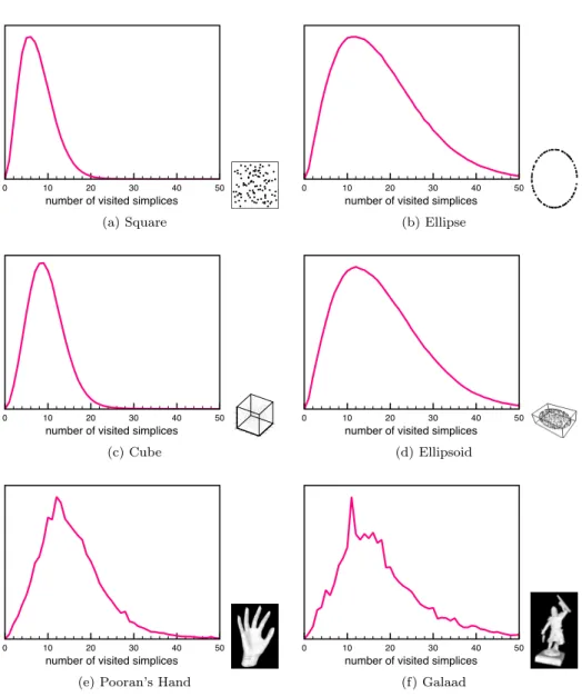
An interesting feature of the Delaunay hierarchy is that the average number of visited simplices during the walk on a particular level of the triangulation tends to be similar for each level when n is big enough. Figure 4 shows the distribution of the number of simplices visited during the stochastic walk done on the last level (level h) of the hierarchy for some set of points. Figure 5 shows experimentally the impact of the number of vertices on the distribution.

3 Predicate Relaxation

The visibility walk assumes that, for every visited simplex s, the next simplex to be visited is a successor of s. The correctness of the algorithm relies on the exactness of the orientation predicates. On one hand, the filtering mecha-nism accelerates the exact orientation test computations (see Section 2.2). On the other hand, the filtering mechanism is slower than the direct orientation test computation through inexact number types (such as e.g., double-precision floating-point numbers). In this section, we propose to extend this filtering mechanism to another level. Instead of just filtering the orientation predicate computations, we also filter the exact stochastic walk (the one relying on exact orientation predicates) by an inexact version of the walk using the orientation predicate computed with inexact type, and thus avoiding the filtering mecha-nism overhead.

(11)

0 10 20 30 40 50

number of visited simplices

(a) Square

0 10 20 30 40 50

(b) Ellipse

0 10 20 30 40 50

0.0 0.25 0.0 1.00.75 0.5 0.25 0.5 0.75 0.5 0.25 1.0 0.75 0.0 1.0 (c) Cube 0 10 20 30 40 50

(d) Ellipsoid

0 10 20 30 40 50

(e) Pooran’s Hand

0 10 20 30 40 50

(f) Galaad

Figure 4: Delaunay hierarchy with stochastic walk. The distribution of the number of simplices visited during the stochastic walk done on the last level of the hierarchy for 220

points: (a) evenly distributed in a square, (b) evenly distributed on an ellipse, (c) evenly distributed in a cube, (d) evenly distributed on an ellipsoid, (e) on Pooran’s Hand model, (f) on Galaad model. The two last models are taken from a laser scan.

The stochastic walk is mostly dependent on the performance of the orienta-tion test, i.e. improving it also improves the whole stochastic walk performance. Allowing the orientation test to be done with inexact type, such as a double type, instead of an exact type: (i) on one hand, makes the computations faster; (ii) on the other hand, makes the computations possibly wrong. Using the stochastic walk with an inexact orientation test might increase the number of visited simplices (even up to an infinite number). In practice however, using

(12)

0 10 20 30 40 50

size of the walk

0 0.02 0.04 0.06 0.08 0.1 0.12 N = 220 N = 212 N = 213 (a) Square 0 10 20 30 40 50

size of the walk

0 0.02 0.04 0.06 0.08 N = 220 N = 212 N = 210 N = 215 (b) Ellipse 0 10 20 30 40 50

size of the walk

0 0.02 0.04 0.06 0.08 0.1 N = 220 N = 212 N = 210 0.0 0.25 0.0 1.00.75 0.5 0.25 0.5 0.75 0.5 0.25 1.0 0.75 0.0 1.0 (c) Cube 0 10 20 30 40 50

size of the walk

0 0.02 0.04 0.06 0.08 N = 2 N = 2 N = 2 10 12 20 15 N = 2 (d) Ellipsoid

Figure 5: Varying the number of vertices. The distribution of the number of simplices visited during the stochastic walk done on the last level of the hierarchy for various number of random points: (a) evenly distributed in a square, and (b) evenly distributed on an ellipse, (c) evenly distributed in a cube, and (d) evenly distributed on an ellipsoid.

doubletype makes almost none of the orientation tests ever give wrong results. Therefore, a two-steps exact algorithm can be designed, where:

• The first step consists into running the stochastic walk algorithm with inexact arithmetics. To avoid a worst-case too big (sometime endless) first step, it is forced to stop after visiting a fixed maximum number of simplices. This step is called the relaxation step, and (i) it has a parameter which is the maximum number of visited simplices, (ii) it returns a simplex (hopefully) not too far from the solution.

• The second step consists into running the stochastic walk algorithm with exact arithmetics from the simplex returned by the relaxation step, until the solution is found. We will call this step the solution step.

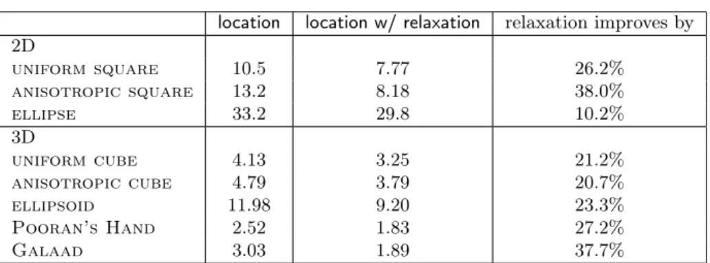
Using this technique with a maximum of 2000 visited simplices in the relax-ation step, leads to an average of 10-40 % improvement on the performance of the stochastic walk in both two and three dimensions for several input sets, see Table 1. This approach improves performance while still benefiting from the robustness of thee exact computing paradigm.

4 Termination Guessing

In this section, we propose another improvement, which works when you have a suitable estimation on the distribution of the number of visited cells by the

(13)

location location w/ relaxation relaxation improves by 2D uniform square 10.5 7.77 26.2% anisotropic square 13.2 8.18 38.0% ellipse 33.2 29.8 10.2% 3D uniform cube 4.13 3.25 21.2% anisotropic cube 4.79 3.79 20.7% ellipsoid 11.98 9.20 23.3% Pooran’s Hand 2.52 1.83 27.2% Galaad 3.03 1.89 37.7%

Table 1: Improving performance with relaxation. All the models have 220

points. The time is computed in seconds and accounts for 215

random queries inside the convex hull of the input points. location corresponds to the stochastic walk algorithm (the solution step), and location w/ relaxation adds the relaxation step into it. In uniform square and uniform cube, points are evenly distributed in the unit square and cube respectively. In anisotropic square and anisotropic cube, points are distributed in the unit square and cube respectively, such that the density ρ ∼ x2

. In ellipse and ellipsoid, points are evenly distributed on an ellipse and ellipsoid. Pooran’s Handand Galaad are real-life 3D models taken from a laser scan.

stochastic walk. This section describes only the two-dimensional case. Not only because it is simpler and extends easily, but also because it is the only dimension where we can get a significant improvement.

Suppose that the total number x of triangles visited by a stochastic walk (see Section 2.1) is known in advance. Then, during the walk, as long as the current triangle being visited t is not yet the x-th, there is no need to test if the last adjacent triangle in the sequence is a successor of t. Instead, it is directly assumed to be a successor of t. In this case, the expected number of orientation tests decreases.

However, supposing a priori knowledge on the total number of visited tri-angles during a stochastic walk, is not realistic. Instead, we “guess” a value x0,

which is (hopefully) close to x. With this in mind, the standard stochastic walk algorithm can be modified as follows: (i) Guessing Phase, a constant number x0 of triangles are visited taking into account the additional assumption that

the last triangle in the sequence is directly a successor (even though this might be a wrong guess), and (ii) Finding Phase, the remaining triangles are visited with a standard stochastic walk. In other words, let t0 be the current triangle

being visited, t−1the previous visited triangle and t1, t2the two other neighbors

of t0. One step of both Guessing Phase and Finding Phase starts by choosing

randomly one of the two triangles t1and t2. Suppose that t1is the first triangle

chosen in the random order, and t2 the second respectively. Then one step in

both Guessing Phase and Finding Phase checks whether t1 is a successor of

t0 in VG and continue the walk in case of success. The difference lies in case

of failure: A step in the Guessing Phase directly continues the walk with t2;

whereas a step in the Finding Phase checks whether t2 is actually a successor

of t0to decide whether to stop walking or not. To simplify descriptions in what

(14)

follows, we denote t−1 by the discarded neighbor

4_{of t}

0, t1 by the first neighbor

of t0, and t2 by the second neighbor of t0.

Naturally, the performance of this modification depends on the quality of the guess. More precisely: (i) if x0 < x, the performance can only be better

than the standard stochastic walk’s performance, i.e. x0steps with the modified

stochastic walk and x−x0steps with the standard stochastic walk; (ii) otherwise,

the x0first steps use the modified stochastic walk, but goes further than x, and

hence some triangles are additionally visited to reach the goal again with the standard stochastic walk. Two exceptions need to be taken into account:

Hitting the convex hull. If during the Guessing Phase, we reach an infinite triangle t0 from a triangle t−1, then we passed through a facet of the

convex hull. In this case, if t0 is: (i) the first neighbor of t−1, then q is outside

the convex hull; (ii) the second neighbor of t−1, then we check if t0is a successor

of t−1. If t0is indeed a successor of t−1, then again q is outside the convex hull;

otherwise, the Finding Phase begins from t−1.

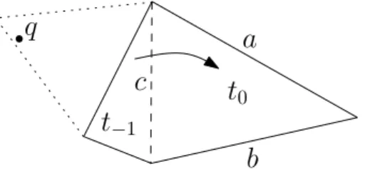
Remembering previously visited triangle. As described before, when visiting a triangle t0 from a triangle t−1, t−1 is a discarded neighbor of t0,

and thus it is not considered as a possible next triangle to visit. Suppose the algorithm is switching from the Guessing Phase to the Finding Phase. When the only successor of t0in VG is exactly t−1(visited during the Guessing Phase), the

algorithm might deduce wrongly that t0contains q, see Figure 6. This happens

because t−1is discarded from the list of potential next triangles to visit. To fix

this, it is sufficient to not discard t−1when switching from the Guessing Phase

to the Finding Phase. Since we assume that x0 is chosen to be smaller than

x, it is reasonable to make t−1 the last one amongst the neighbors of t0 to be

tested.

q

_a

b

t

₋₁

t

0

c

Figure 6: Switching from the Guessing Phase to the Finding Phase.

After x0 steps, termination guessing stops at t. The previously visited triangle and t share edge c. In the next step: the adjacent triangles of t with common edges a and b are not successors of t; the only alternative is the previous visited triangle, but it is skipped, and thus, the triangle is wrongly deduced to be containing q.

Given x and x0 > 0, the expected amount of orientation tests depends on

the number of successors per visited triangle during the walk. We will evaluate now, the expected total number of orientation tests computed by the modified stochastic walk. Suppose, the following two scenarios where q is in the interior of the convex hull of the domain:

Points on two parallel lines. In this case, for each triangle t during the walk, there is: (i) one adjacent triangle which has been visited, (ii) one adjacent

4

The meaning of the word “discard” here, is that the neighbor is discarded from the possible candidates to be visited next.

(15)

triangle which is infinite, and (iii) one adjacent triangle which is closer to q. And thus, for each t, there are only one successor. In the first step, we need to do an expected number of at most 5/3 orientation tests: 1/3 probability that the first, second and third adjacent triangle is a successor of t respectively5_.

In the next x0− 1 steps, as we remember the previously visited triangle, and

we use termination guessing, we have exactly x0− 1 orientation tests to do.

Now, we will pessimistically assume that if x0 goes x − x0steps away from the

cell containing the query, then it will take x − x0 additional steps to return

back. In this case, as we are not doing termination guessing anymore, there is 1/2 probability that the first adjacent triangle checked is a successor of t, and 1/2 probability that the last one is a successor of t. That gives an expected 3/2 × |x − x0| expected orientation test computations. We can summarize this

as follows. In the case of points on two parallel lines, for a given x, the expected total number of orientation tests computed by the modified stochastic walk, using x0 as guess, is given by:

F (x, x0) = x0+

2 3 +

3

2|x − x0|. (2)

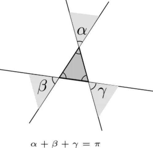
Points on an ellipsoid with different axis size should follow the same analysis. Points uniformly distributed in the unit cube. In this case, for each triangle t during the walk, considering that q is sufficiently far away from s, there is a 1/2 probability that t has only one successor, see Figure 7.

α

β

_γ

α + β + γ = π

Figure 7: Number of successors. If q is inside the light-grey regions, then the number N of successors of t is 2. Otherwise, N = 1. If q is far from t, the probability that N = 2 is approximately the sum of the angles divided by the total angle of the unit circle, i.e. π/2π = 1/2.

The same analysis as above gives that, in the case of points evenly distributed in the unit square, for a given x, the expected total number of orientation tests computed by the modified stochastic walk, using x0as guess, is given by:

F (x, x0) = x0+ 2 3 + 5 4|x − x0|. (3) 5

As we are using termination guessing, when the first triangle is not a successor of t, we check only one additional adjacent triangle to be a successor of t. And thus, we have 5/3 = 1/3 × 1 + 2/3 × 2 expected orientation test computations.

(16)

Now, suppose that x is a random variable with distribution P (x) for x ∈ N. Then, for a given x0, the expected total number of orientation test computations

is given by E(x0) = ∞ X i=0 F (x, x0) · P (x). (4)

And then, the best guess x∗_{, is given by x}∗_{= arg min}

i∈NE(i).

Again, it is not realistic to assume that P is known. However in this case, the distribution P can be estimated on-line by updating a histogram with the total number of visited triangles per query. When the estimation is (heuristically) good enough, then x∗ _{is computed, and the modified stochastic walk is used}

instead. Computing x∗ _{can be done efficiently by a binary search on E(x),}

since E has only one minimum. Figure 8 shows x∗ _{for the case of points evenly}

distributed in the unit square, and points following the distribution ρ(x, y) = x2

in the unit square.

1100 1150 1200 1250 value of x 0 19.36% less orientation tests x* = 1149 (a) uniform 950 1000 1050 1100 value of x 0 19.28% less orientation tests x* = 1003 (b) ρ = x2

Figure 8: A bound on the expected number of orientation tests in function of x0. The distribution is computed, then E(x0) is estimated for points: (i) evenly distributed in the unit square, (ii) following the distribution ρ(x, y) = x2

in the unit square.

We implemented this algorithm in both two and three dimensions, and the actual number of orientation tests computed, for several inputs, are summarized in Figure 9.

In Figure 8, the value of x∗ _{obtained by Eq.(3), Eq.(4), and P (computed}

experimentally) coincides with the value of x∗ _{obtained when running the}

im-plementation in Figure 9, for points evenly distributed in the unit square. We can see that the bound in Figure 8 is rather pessimistic compared with what happens in practice. Also from Figure 8, in 2D, the number of orientation tests computed is considerably smaller when using the termination guessing (around 25%); specially in the case of points on an ellipse which is in accord with the theory, since the standard stochastic walk is less efficient (3/2 orientation tests per triangles visited in average for points an ellipse, and only 5/4 orientation tests per triangles for points evenly distributed in the square). As E(x0) is

monotonically decreasing for x0 ≤ x∗, then for any x0 ≤ x∗ the performance

is better than the standard stochastic walk (x0 = 0). And hence, e.g., just

skipping the last few orientation tests, leads to a speed-up.

(17)

14 P. de Castro & O. Devillers 0 200 400 600 800 1000 1200 1400 value of x 1200 1300 1400 1500 1600 n u mb e r o f o ri e n ta ti o n t e st s 0 Minimum at 1149 24.3% less orientation tests

0 200 400 600 800 1000 1200 1400 value of x 1000 1100 1200 1300 1400 1500 n u mb e r o f o ri e n ta ti o n t e st s 0 Minimum at 940 24.8% less orientation tests

0 2000 4000 6000 8000 10000 value of x 7000 8000 9000 10000 11000 12000 n u mb e r o f o ri e n ta ti o n t e st s 0 Minimum at 7164 33.28% less orientation tests

(a) 2D 0 50 100 150 200 250 300 value of x 320 340 360 380 400 420 440 n u mb e r o f o ri e n ta ti o n t e st s 0 Minimum at 153 4.90% less orientation tests

0 50 100 150 200 250 300 value of x 300 320 340 360 380 400 420 440 460 n u mb e r o f o ri e n ta ti o n t e st s 0 Minimum at 198 4.97% less orientation tests

0 200 400 600 800 1000 12001400 value of x 1420 1440 1460 1480 1500 1520 1540 n u mb e r o f o ri e n ta ti o n t e st s 0 Minimum at 928 6.14% less orientation tests

(b) 3D

Figure 9: Actual number of orientation tests per x0 with termination

guessing. The figure above shows the actual number of orientation tests computed with termination guessing for various values of x0, in a Delaunay triangulations of 2

20 points: (a) left, evenly distributed in the unit square; center, following the distribution ρ(x, y) = x2

in the unit square; right, evenly distributed on an ellipse; (b) left, evenly distributed in the unit cube; center, following the distribution ρ(x, y, z) = x2

in the unit cube; right, evenly distributed on an ellipsoid. For (a), the query is located in (1/2, 3/4) and starts from the triangle enclosing (1/2, 1/4); for (b), the query is located in (1/2, 1/2, 3/4) and starts from the tetrahedron enclosing (1/2, 1/2, 1/4).

Choosing a small value of x0 (such as 2 or 3), should be useful for

Delau-nay hierarchies, since, as shown in Figures 4 and 5, the distribution of visited triangles is concentrated in low values of x for different values of n. However, ex-periments showed that the improvement in this case is rather weak, and hardly represent more than 5% of the total time.

5 Conclusions

We proposed two modifications of the stochastic walk strategy which improves performance up to a factor of 40%. Both modifications are practical and simple to implement. Also, if the predicate relaxation works well for an input set, then the performance gains of the two methods are cumulative. We will submit the predication relaxation for integration in the library. As the termination guessing needs fine-tuning and Cgal is a general purpose library, we decide to not submit it yet.

Unfortunately, little are known about the exact distributions of the stochas-tic walk (even tight bound on the average). We wish to mention this theorestochas-tical advancement as a well-suited future work.

(18)

Acknowledgments The authors wish to thank Aim@shape for providing the realistic models, ANR Project Triangles and Région PACA for their support.

References

[1] P. Bose and L. Devroye. Intersections with random geometric objects. Technical report, School of Computer Science, McGill University, 1995. Manuscript.

[2] CGAL Editorial Board. CGAL User and Reference Manual, 3.5 edition, 2009. www.cgal.org.

[3] Olivier Devillers. The Delaunay hierarchy. Internat. J. Found. Comput. Sci., 13:163–180, 2002.

[4] Olivier Devillers, Sylvain Pion, and Monique Teillaud. Walking in a trian-gulation. Internat. J. Found. Comput. Sci., 13:181–199, 2002.

[5] Luc Devroye, Christophe Lemaire, and Jean-Michel Moreau. Expected time analysis for Delaunay point location. Comput. Geom. Theory Appl., 29:61–89, 2004.

[6] J. E. Goodman and J. O’Rourke, editors. Handbook of Discrete and Com-putational Geometry. CRC Press LLC, Boca Raton, FL, 2004. 2nd edition. [7] Lutz Kettner, Kurt Mehlhorn, Sylvain Pion, Stefan Schirra, and Chee Yap. Classroom examples of robustness problems in geometric computations. In Proc. 12th European Symposium on Algorithms, volume 3221 of Lecture Notes Comput. Sci., pages 702–713. Springer-Verlag, 2004.

[8] D. G. Kirkpatrick. Optimal search in planar subdivisions. SIAM J. Com-put., 12(1):28–35, 1983.

[9] Ernst P. Mücke, Isaac Saias, and Binhai Zhu. Fast randomized point loca-tion without preprocessing in two- and three-dimensional Delaunay trian-gulations. In Proc. 12th Annu. Sympos. Comput. Geom., pages 274–283, 1996.

[10] Sylvain Pion and Monique Teillaud. 3D triangulations. In CGAL Editorial Board, editor, CGAL User and Reference Manual. 3.5 edition, 2009. [11] C. K. Yap and T. Dubé. The exact computation paradigm. In D.-Z. Du

and F. K. Hwang, editors, Computing in Euclidean Geometry, volume 4 of Lecture Notes Series on Computing, pages 452–492. World Scientific, Singapore, 2nd edition, 1995.

[12] Mariette Yvinec. 2D triangulations. In CGAL Editorial Board, editor, CGAL User and Reference Manual. 3.5 edition, 2009.

(19)

Centre de recherche INRIA Sophia Antipolis – Méditerranée 2004, route des Lucioles - BP 93 - 06902 Sophia Antipolis Cedex (France)

Centre de recherche INRIA Bordeaux – Sud Ouest : Domaine Universitaire - 351, cours de la Libération - 33405 Talence Cedex Centre de recherche INRIA Grenoble – Rhône-Alpes : 655, avenue de l’Europe - 38334 Montbonnot Saint-Ismier Centre de recherche INRIA Lille – Nord Europe : Parc Scientifique de la Haute Borne - 40, avenue Halley - 59650 Villeneuve d’Ascq

Centre de recherche INRIA Nancy – Grand Est : LORIA, Technopôle de Nancy-Brabois - Campus scientifique 615, rue du Jardin Botanique - BP 101 - 54602 Villers-lès-Nancy Cedex

Centre de recherche INRIA Paris – Rocquencourt : Domaine de Voluceau - Rocquencourt - BP 105 - 78153 Le Chesnay Cedex Centre de recherche INRIA Rennes – Bretagne Atlantique : IRISA, Campus universitaire de Beaulieu - 35042 Rennes Cedex Centre de recherche INRIA Saclay – Île-de-France : Parc Orsay Université - ZAC des Vignes : 4, rue Jacques Monod - 91893 Orsay Cedex

Éditeur

INRIA - Domaine de Voluceau - Rocquencourt, BP 105 - 78153 Le Chesnay Cedex (France)

http://www.inria.fr ISSN 0249-6399