HAL Id: hal-02330920
https://hal.archives-ouvertes.fr/hal-02330920
Submitted on 24 Oct 2019
HAL is a multi-disciplinary open access archive for the deposit and dissemination of sci-entific research documents, whether they are pub-lished or not. The documents may come from teaching and research institutions in France or abroad, or from public or private research centers.
L’archive ouverte pluridisciplinaire HAL, est destinée au dépôt et à la diffusion de documents scientifiques de niveau recherche, publiés ou non, émanant des établissements d’enseignement et de recherche français ou étrangers, des laboratoires publics ou privés.
A second-order realizable scheme for moment advection
on unstructured grids
Alberto Passalacqua, Frédérique Laurent, Rodney Fox
To cite this version:
Alberto Passalacqua, Frédérique Laurent, Rodney Fox. A second-order realizable scheme for moment advection on unstructured grids. Computer Physics Communications, Elsevier, 2020, 248, pp.106993. �10.1016/j.cpc.2019.106993�. �hal-02330920�
Preprint submitted to Elsevier
A second-order realizable scheme for moment advection on
unstructured grids
Alberto Passalacquaa, b, d *, Frédérique Laurentb, c, Rodney O. Foxd
aDepartment of Mechanical Engineering, Iowa State University, Black Engineering Building, Ames, IA 50011, USA bLaboratoire EM2C, CNRS, CentraleSupélec, 3 rue Joliot Curie, Bâtiment Eiffel, 91190 Gif-sur-Yvette, France
cFédération de Mathématiques de l'Ecole Centrale Paris, FR CNRS 3487, France
dDepartment of Chemical and Biological Engineering, Iowa State University, Sweeney Hall, Ames, IA, 50011-2230, USA
Abstract
The second-order realizable 𝜁 moment advection scheme developed in Laurent and Nguyen, (2017) is extended to the case of unstructured grids with cells of arbitrary shape. The necessary modifications to the scheme and the conditions under which the scheme ensures the realizability of the advected moment set are presented. The implementation of the scheme in the OpenFOAM® CFD toolbox is verified comparing the results obtained in one-dimensional test cases involving moment sets well inside the moment space, and at the boundary of the moment space. Results obtained with the proposed scheme are compared to the corresponding analytical solution. The scheme is then tested considering two-dimensional cases of pure moment advection with an imposed irrotational velocity field. First, a quadrilateral grid is considered to determine the order of the scheme and compare it to the results reported in Laurent and Nguyen (2017) with the same grid resolution. Then, the accuracy of the scheme on two-dimensional triangular grids is determined.
Keywords: Moment advection, realizability, unstructured grid, advection, schemes, moment methods,
quadrature method of moments
1. Introduction
Moment methods are a class of mathematical methods used to determine approximate solutions to
* Corresponding author
2
problems involving the evolution of a distribution function. Notable examples of equations describing this evolution are the population balance equation [2,3], the Boltzmann [4,5], the Boltzmann-Enskog [2], the Fokker-Planck and Kolmogorov [6–8] equations, in addition to several others. These equations can be written in compact form as
𝜕𝑓
𝜕𝑡 + ∇𝐱⋅ (𝑓𝐯) + 𝒮 = 0 (1.1)
where 𝑓(𝑡, 𝐱, 𝛏) is the distribution, 𝐱 is the position vector, 𝛏 is the vector of internal coordinates specific to the problem (e.g. size, composition, velocity, charge…), 𝐯 is the velocity and 𝒮 contains other terms depending on the evolution equation for 𝑓 under consideration.
Moment methods [9–11] consist in deriving partial differential equations (PDEs) for the spatio-temporal evolution of a finite vector of moments of the distribution function characteristic of the problem under consideration, in order to reduce the dimensionality of the problem and, consequently, make it computationally more treatable. This is achieved by applying the definition of moment of 𝑓
𝑚𝑖𝑗𝑘… = ∫ 𝜉1𝑖𝜉2 𝑗
𝜉3𝑘… 𝑓𝑡, 𝐱, 𝛏)d𝛏
Ω
(1.2) to both sides of Eq. (1.1), which leads to conservation equations for the quantities 𝑚𝑖𝑗𝑘…, which are
the moments about the origin of 𝑓. The PDEs obtained in this way are then discretized on the domain of interest and solved numerically, typically using the finite-volume method [12,13]. The literature reports many example applications where moment methods were used [9,10,14–43], including applications to aerosols [11,17,18], gas-particle flows [37,44,45], gas-liquid flows [22,22,39,46], combustion [27,43,47], sprays [24,32,35,48] and radiation transport [14], to mention a few. In this work we focus on the transport of moments of a univariate distribution, where 𝛏 contains only one scalar positive quantity, as it happens in the solution of population balance equations describing the evolution of the particle size in a particle population.
A key difficulty in formulating numerical methods for the solution of PDEs describing the evolution of a moment vector is the discretization of the advection term. As illustrated by Wright [49], this difficulty consists in preserving the moment realizability2, which is systematically compromised if classical discretization schemes, different from first-order upwind, are used to discretize the advection
2 A moment vector is said realizable on a support if a positive measure exists on the same support whose moments are
3
term [49]. The first-order upwind scheme, while used in most of the applications of moment methods found in the literature in order to avoid compromising moment realizability, is too dissipative, and requires extremely refined grid resolutions to achieve satisfactory results, seriously compromising the feasibility of simulations in applications involving large-scale domains or large gradients of the transported moment vector. Wright [49] examined several solutions to the problem of moment corruption due to advection, including the adoption of augmented schemes for vector transport, the transport of surrogate quantities related to the moment vector that needs to be advected, of quadrature weights and abscissae associated to the moment set in certain quadrature-based moment methods [50], and moment correction algorithms [49,51]. This latter approach consists in replacing the compromised moment vector with a valid one, obtained either by removing negative second-order differences [3] or enacting an optimization procedure to identify a moment vector that maximized ln 𝑚𝑘 [51].
Kah et al. [32] developed a second-order realizable advection scheme for moment vectors of distribution with compact support, suitable for structured grids, in cases with moment vectors in the interior of the moment space. In their approach, instead of performing a direct spatial reconstruction of the moment vector of interest, the corresponding vector of canonical moments is considered. The boundedness of the canonical moments, which are necessarily positive scalars defined over ]0, 1[ is leveraged to formulate a limiter which ensures not only the boundedness of the numerical solution, but also the realizability of the vector of transported moments under a condition on the integration time step. The resulting scheme was applied together with adaptive mesh refinement in [52].
Vikas et al. [53] proposed a quasi-high-order realizable advection scheme in the context of quadrature-based moment methods. In their scheme, which was formulated on unstructured grids, the advection term is computed as a function of the quadrature approximation of the NDF [3,11], using a MUSCL-type limited scheme for the reconstruction of the quadrature weights and a first-order upwind scheme for quadrature abscissae. The scheme ensures moment realizability if a condition on the integration time-step is satisfied. However, the formal order of accuracy of the scheme is limited by the first-order reconstruction of the quadrature abscissae. Vikas et al. [54] proposed a realizable scheme for diffusion problems, always in the context of quadrature-based moment methods.
Alldredge and Schneider [55] formulated a discontinuous Galerkin scheme in the context of entropy-based moment closures, coupling it with a strong stability preserving Runge-Kutta method for time integration. Since this approach relies on entropy-based closures, it is suitable for problems with moment vectors in the interior of the moment space but does not deal with the case of moment
4 vectors are the boundary of the moment space.
Laurent and Nguyen [1] developed a second-order realizable scheme by considering the reconstruction of positive quantities related to the set of transported moments in what they have called 𝜁 scheme. This numerical scheme, which requires a CFL-like condition to ensure the realizability of the moment vector, was successfully applied to the transport of moment vectors of a regular NDF and of a bimodal NDF, with moments possibly at the boundary of the moment space. In both cases the scheme has shown the capability of preserving the realizability of the advected moment vector, while maintaining its accuracy.
The nature of the 𝜁 scheme and, in particular, the version of this scheme called 𝜁 simplified scheme by Laurent and Nguyen [1], makes it an ideal candidate for its extension to unstructured grids with cells of arbitrary shapes because the scheme relies on a traditional MUSCL reconstruction, and only requires a local additional limitation to be applied to the reconstructed quantities on cell faces. The extension of this scheme to unstructured grids and its implementation into the OpenFOAM framework [56] are the topics of this article, the remainder of which is organized as follows: in Sec. 2 the problem of moment transport is introduced. The 𝜁 simplified scheme for hexahedral structured grids of Laurent and Nguyen [1] is summarized in Sec. 3. Its generalization to unstructured grids with cells of arbitrary shapes is discussed in Sec. 4. Finally, the same one- and two-dimensional test cases used by Laurent and Nguyen [1] are used in Sec. 5 to verify the implementation of the numerical scheme, using hexahedral uniform grids. Then, the two-dimensional cases are repeated using a triangular grid, and the order of accuracy of the 𝜁 simplified scheme on unstructured grids is assessed.
2. Moment transport and moment advection
The focus of the present work is on the pure advection problem of a moment vector 𝐦N =
(𝑚0, … , 𝑚N−1) associated to a measure with support over ℝ+, with a known velocity field 𝐔,
according to the set of equations 𝜕𝑚𝑘
𝜕𝑡 + ∇𝐱⋅ (𝑚𝑘𝐔) = 0, ∀𝑚𝑘∈ 𝐦N. (2.1)
The solution of Eq. (2.1) is non-trivial because the numerical schemes used to discretize the time derivative and the divergence term need to guarantee the moment vector 𝐦N remains realizable. This
5
satisfy. These conditions are represented, for moments associated to a measure with support on ℝ+,
through the Hankel determinants [57,58]:
𝐻2𝑝 = | 𝑚0 … 𝑚𝑝 ⋮ ⋱ ⋮ 𝑚𝑝 … 𝑚2𝑝| , 𝐻2𝑝+1 = | 𝑚1 … 𝑚𝑝+1 ⋮ ⋱ ⋮ 𝑚𝑝+1 … 𝑚2𝑝+1|, (2.2) with 𝐻−2 = 𝐻−1= 1.
Necessary and sufficient condition for 𝐦N to be in the interior of the moment space is that 𝐻2𝑝 > 0
and 𝐻2𝑝+1 > 0. Moreover, when 𝐦N is at the boundary of the moment space, some of these Hankel
determinants are null.
A discussion on realizable time integration schemes can be found, for example, in [53]. Since the focus of this article is on advection schemes, it suffices to remember that any time-integration scheme convex combination of explicit Euler steps is realizable under some restriction on the integration time step.
As anticipated in the introduction, the objective of this article is to extend the second-order realizable advection scheme of Laurent and Nguyen [1] to unstructured grids. To such a purpose, let us consider a computational grid made of cells of arbitrary shape. The volume of a generic cell c is Ωc, and the
number of faces of the same cell is Nf,𝑐. The subscript own indicates the reconstructed values of a
variable at the cell face, assuming outgoing flux; the subscript nei indicates the reconstructed values of a variable at the cell face if the flux is going into the cell. For consistency with the convention adopted in OpenFOAM, we assume the flux of a transported property to be positive when outgoing with respect to the computational cell owning the face used to define the flux.
Following Vikas et al. [53], and using the nomenclature introduced above, Eq. (2.1) can be rewritten in semi-discrete form to obtain the evolution equation of the moment 𝑚𝑘 defined at the center of
each computational cells. Such equation reads 𝜕𝑚𝑘,𝑐
𝜕𝑡 + 1 Ω𝑐
∑ [𝑚𝑘,own,𝑓max(𝐔𝑓⋅ 𝐒𝑓, 0) + 𝑚𝑘,nei,𝑓min(𝐔𝑓⋅ 𝐒𝑓, 0)] = 0 Nf,𝑐−1
𝑓=0
, (2.3) where 𝐒𝑓 is the vector normal to the surface of the cell face 𝑓, belonging to cell 𝑐, with magnitude
equal to the surface area of the cell face |𝐒𝑓| and pointing outward of the cell, and 𝐔𝑓 is the
6
A procedure needs to be developed to compute the moments 𝑚𝑘,own,𝑓 and 𝑚𝑘,nei,𝑓 to ensure the
realizability of the advected moment vector 𝐦N because, as discussed in the introduction, conventional finite-volume advection schemes, relying on reconstructions of order higher than one, do not guarantee the realizability of the transported moment set [49].
3. The simplified 𝜻 advection scheme
This section summarizes the realizable 𝜁 simplified advection scheme [1], which represents the foundation of the scheme for unstructured grids subject of the present work. This scheme was developed for one-dimensional problems with uniform spatial discretization and extended to multiple dimensional problems with Cartesian grids through dimensional splitting. Only the one-dimensional scheme is presented here.
In the 𝜁 simplified scheme, the moment vector 𝐦N is advected by considering the auxiliary vector
𝛇N−1 = (𝜁0, … , 𝜁𝑁−2), with
𝜁𝑝 = 𝐻𝑝+1𝐻𝑝−2
𝐻𝑝𝐻𝑝−1 , 𝑝 = 0, 1, … , N − 2, (3.1)
where 𝐻2𝑝 and 𝐻2𝑝+1 are the Hankel determinants in Eq. (1.2).
These quantities are efficiently calculated using the QD algorithm [57], the Chebychev algorithm [1] or the Wheeler algorithm [59]. The adoption of the last two approaches is particularly convenient in the context of quadrature-based moment methods because the coefficients required to calculate the quantities 𝜁𝑝 correspond to the coefficients of the recurrence relationship of the orthogonal
polynomials used to determine the quadrature formula.
Once the vector 𝛇N−1 has been defined, the 𝜁 simplified advection scheme consists of the following
steps:
1. The zero-order moment 𝑚0 is advected using a conventional MUSCL scheme with the
minmod limiter.
2. The values of 𝜁𝑝 are reconstructed at each side of each cell face using the same MUSCL-type
reconstruction as for 𝑚0, which ensures the positivity of the quantities 𝜁𝑝 is preserved. 3. An additional limitation is conditionally applied to the slopes used to perform the
7
moment set. This additional limitation is defined based on the realizability of the moment vector [1,60]
𝐦∗ = 3𝐦 − 𝐦+− 𝐦−, (3.2)
where 𝐦 is the moment vector at the cell center, 𝐦+ and 𝐦− are the moment vectors
computed from the values 𝜁𝑝+ and 𝜁
𝑝− reconstructed at cell faces. If the moment vector defined
by Eq. (3.2) is not realizable, an iterative procedure is used to reduce the slopes used to reconstruct 𝜁𝑝 on cell faces, to ensure the realizability of the moment vector at the cost of the accuracy of the reconstruction. Details of this procedure are reported in Laurent and Nguyen (2017), and its generalization to unstructured grids is discussed in this work.
4. Once the reconstructed face values of 𝜁𝑝 which ensure the realizability of the entire advected
moment set are found, the moment vectors 𝐦+ and 𝐦− are recomputed from the values ζ 𝑝 +
and ζ𝑝− [61].
5. The integration of the advection term proceeds computing the flux of each moment at each cell face based on the direction of the velocity at the centroid of the same face and updating the values of the moments at the cell center, as prescribed by Eq. (2.3).
The scheme summarized above was proven [1] to preserve the realizability of the advected moment vector if the time step is adapted to maintain the value of the CFL number below 1/3, while converging to second-order accuracy with a sufficiently refined spatial discretization.
The extension of the 𝜁 simplified scheme to unstructured grids requires the generalization of the definition of 𝐦∗ in Eq. (3.2), and of the CFL condition, which is expected to become a function of
the number of faces of the grid cell.
4. Generalization to unstructured grids
The generalization of the 𝜁 simplified scheme to unstructured grids is achieved in this work by considering a co-located grid arrangement, where all the variables are stored at cell centroids, with the exclusion of the values at the boundary of the computational domain, where values are stored at face centroids. This approach is illustrated, for example, in Ferziger and Peric [13], and was adopted in the computational toolkit [56,62,63] used in this work.
8
the velocity and of the advected quantities need to be known at cell faces. The reconstruction of the advected scalars, moments in our case, is illustrated in Sec. 4.1, following the approach implemented into OpenFOAM [56,62], based on the work of several authors [64–70] and summarized by Darwish and Moukalled [71].
4.1. Reconstruction on unstructured grids
Let us consider a generic advected quantity whose value, stored at the centroid C of a generic cell of the computational mesh, is indicated with 𝜓C. The value of 𝜓 reconstructed on the cell face f is [67,71]
𝜓f= 𝜓C+1
2ℒ(𝑟f)(𝜓D− 𝜓C), (4.1)
where ℒ(𝑟f) is the limiter function, which depends on the ratio [71] 𝑟f =
2∇𝜓C⋅ 𝐫CD 𝜓D− 𝜓C
− 1, (4.2)
with 𝑟𝑓≥ 0 for TVD schemes [71].
In these expressions, 𝜓D represents the downwind value at the center of the neighbor cell sharing face f with the cell whose center is situated in C. The vector 𝐫CD joins the centers C and D of the same two
neighbor cells. The definition of the limiter function for a minmod limiter is [66,71]:
ℒ(𝑟f) = max(0, min(1, 𝑟f)). (4.3)
The evaluation of the gradient of 𝜓 over the cell C in Eq. (4.2) is detailed in Darwish and Moukalled [71]. A second-order least-squares method is used in this work to ensure accuracy on grids with cells of arbitrary shape and non-uniform spatial distribution.
4.2. Additional limitation for moment sets at the boundary of the moment space
The condition in Eq. (3.2), used to identify cases when an additional limitation is needed for the reconstructed values of the quantities 𝜁𝑝, needs to be generalized to be applicable to unstructured
grids. To this purpose, let Nf be the maximum number of faces of a cell of the computational grid.
Since arbitrary shaped cells are considered, this value can be different for any cell, without additional complication of the numerical scheme. Let also the flux of the quantities be positive when outgoing with respect to the computational cell under consideration. The number of faces characterized by outgoing flux with respect to the owner cell will be indicated with Nf,o,c. The first step required to
9
extend the 𝜁 simplified scheme [1] to unstructured grids consists in computing the value of the zero-order moment 𝑚0 and of the components 𝜁𝑝 of the vector 𝛇N−1 at both sides of each face internal to
the computational domain3. The symbols 𝑚
0,own and 𝑚0,nei are used to indicate the values of 𝑚0
reconstructed, respectively, at the side of the owner and neighbor cell. Similarly, 𝜁𝑝,own and 𝜁𝑝,nei
indicate the values of 𝜁𝑝 at the side of the owner cell and of the neighbor cell to the face, as discussed for 𝑚0.
Once the reconstruction of 𝑚0 and 𝛇N−1 is obtained, the moments at each side of each cell face are
recomputed from the vectors (𝑚0,own, 𝛇N−1,own) and (𝑚0,nei, 𝛇N−1,nei) using the algorithm
proposed by Skibinsky [61].
At this point, it is determined if an additional limitation needs to be applied to the reconstructed values of 𝜁𝑝, to guarantee the realizability of the advected moment set. This is achieved by defining, in each
computational cell 𝑐, the quantity
𝑚𝑘,𝑐+ = ∑ 𝑚𝑘,𝑐,𝑓
Nf,o,c−1
𝑓=0
, (4.4)
where 𝑚𝑘,𝑐,𝑓 = 𝑚𝑘,own,𝑓 is the value of the moment 𝑚𝑘 reconstructed on face 𝑓 of cell 𝑐, where the
flux is outgoing. The quantities 𝑚𝑘,𝑐+ are then used to define the components of the 𝐦∗ vector as
𝑚𝑘,𝑐∗ = (Nf,o,c+ 1)𝑚𝑘,𝑐− 𝑚𝑘,𝑐+ , 𝑘 = 0, … , N − 1. (4.5) If the number of realizable moments in 𝐦∗ is smaller than the number of realizable moments in the
cell, an additional limitation needs to be applied to the reconstructed values of the 𝜁𝑝 quantities. The
procedure is analogous to the one described in [1], which is summarized here in a slightly modified fashion to clarify the details of its implementation into OpenFOAM.
While not strictly necessary, the reconstructed values 𝜁𝑝,f at cell faces are decomposed, for
convenience in the implementation, into the value obtained from a first-order reconstruction 𝜁𝑝,f,up,
and into a high-order correction 𝜁𝑝,f,h.o. This correction is then multiplied by a coefficient 𝜆𝑝,f∈
[0, 1], which is the limiter that needs to be determined to ensure the realizability of the advected
3 Faces of the computational grid are indicated as internal when they do not belong to a boundary of the computational
domain. Values of moments at boundary faces are either known, if imposed at the boundary, or obtained from the only neighbor cell which owns the boundary face.
10 moment set:
𝜁𝑝,f= 𝜁𝑝,f,up+ 𝜆𝑝,f𝜁𝑝,f,h.o.. (4.6) The value of 𝜆𝑝,f is found by considering the values of the limiters determined based on the owner
and the neighbor cell of face f, and taking their minimum:
𝜆𝑝,f = min(𝜆𝑝,own, 𝜆𝑝,nei). (4.7)
In each cell, the value of the limiter 𝜆𝑘,𝑐 is determined as follows:
1. Set 𝜆𝑝,𝑐 = 1.
2. Compute 𝐦𝑐+ using 𝜁𝑙,f with 𝑙 ≤ 𝑘, and with 𝜁𝑝,f,up, for 𝑙 > 𝑝.
3. Recompute 𝐦𝑐∗ using the values of 𝐦𝑐+ found at the previous step.
4. Calculate the number of realizable moments in 𝐦𝑐∗. If this number is smaller than the number
of realizable moments in 𝐦𝑐, set 𝜆𝑝,𝑐 = 1/2. 5. Recompute 𝜁𝑝,𝑐 from Eq. (4.6).
6. Repeat the calculation at points 2 – 4 with the new value of 𝜁𝑝,𝑐. If the number of realizable
moments in the updated 𝐦𝑐∗ is smaller than the number of realizable moments in 𝐦𝑐, set
𝜆𝑝,𝑐 = 0.
7. Repeat from 1 for all 𝑝 to define the limiter for each of the elements of 𝛇N−1.
Once the cell values 𝜆𝑝,𝑐 are defined for each cell, the face limiters are computed according to Eq.
(4.7), and the reconstructed values of 𝛇N−1,own and 𝛇N−1,nei are updated applying Eq. (4.6) to each of
their components. The updated moment vectors 𝐦N−1,own and 𝐦N−1,nei are then found using the
Skibinsky [61] algorithm to account for the additional limitation determined according to the procedure described above. These updated moment sets are used to define the advection term in the moment conservation equations (Eq. (2.3)).
4.3. Courant – Friedrichs - Lewy condition for realizability
The proposed scheme ensures the realizability of the advected moment set if the time step Δ𝑡 used to perform the integration satisfies a CFL condition obtained at the cell faces at which the flux is outgoing. If we consider an arbitrary cell with Nf,c faces, Nf,o,c of which have an outgoing flux, the maximum value of the CFL number is
11 CFLmax= 1 2maxc ( ∑ 𝐔𝑓 𝑓⋅ 𝐒𝑓 𝑉c ) Δ𝑡, (4.8)
where 𝑉c is the cell volume, 𝐔𝑓 the flow velocity at the cell face 𝑓 with surface 𝐒𝑓, belonging to cell c,
and Δ𝑡 is the time step. Using the same notation, the maximum value of the time step to ensure moment realizability is defined by the condition
max 𝑐 [max𝑓 ( 𝐔𝑓⋅ 𝐒𝑓 𝑉𝑐 )] Δ𝑡 ≤ min 1 Nf,o,c+ 1 , (4.9)
where the minimum function on the right-hand side of Eq. (4.9) is introduced to account for the different number of faces cells may have in unstructured grids.
This is proven by considering the moment vector 𝐦N,𝑐𝑛 at time 𝑡
𝑛, and integrate it according to Eq.
(2.3) with a backward Euler step to obtain the updated moment vector 𝐦N,𝑐𝑛+1 at time 𝑡
𝑛+1. Assuming
𝐔𝑓⋅ 𝐒𝑓> 0 for 𝑓 = 1, … , Nf,o,c and 𝐔𝑓⋅ 𝐒𝑓 ≤ 0 for 𝑓 = Nf,o,c, … , Nf,c, it is possible to write:
𝐦N,c𝑛+1 = 𝐦N,c𝑛 −Δ𝑡 𝑉c ∑ 𝐦N,own,𝑓 𝑛 𝐔 𝑓⋅ 𝐒𝑓 Nf,o,c 𝑓=1 ⏟ 𝒜 −Δ𝑡 𝑉c ∑ 𝐦N,c 𝑛 𝐔 𝑓⋅ 𝐒𝑓 Nf,c 𝑓=Nf,o,c+1 ⏟ ℬ . (4.10)
in which only the term 𝒜 is of interest in the proof because ℬ is necessarily realizable. The moment vector 𝐦N,c𝑛 can be expressed in terms of 𝐦c∗
𝐦N,c𝑛 = 1 Nf,o,c+ 1(𝐦c ∗+ ∑ 𝐦 N,own,𝑓 𝑛 Nf,o,c 𝑓=1 ), (4.11) consequently: 𝒜 = 1 Nf,o,c+ 1𝐦c ∗+ ∑ ( 1 Nf,o,c+ 1− Δ𝑡 𝑉c 𝐔𝑓⋅ 𝐒𝑓) 𝐦N,own,𝑓 𝑛 Nf,o,c 𝑓=1 . (4.12)
By imposing the term in the summation is positive to ensure the realizability of the moment vector, the condition
1 Nf,o,c+ 1 ≥
Δ𝑡
𝑉c 𝐔𝑓⋅ 𝐒𝑓 (4.13)
12
It is worth observing that the definition in Eq. (4.9) automatically includes faces internal to the computational domain and faces lying on the boundary. Consequently, no special consideration for boundary conditions where the flux is imposed is needed to correctly define the maximum CFL required to ensure moment realizability.
The condition in Eq. (4.13) reduces, in the case of a uniform one-dimensional discretization with step Δ𝑥, to
Δ𝑡 ≤ Δx
2𝑈𝑓 (4.14)
because Nf,o,c = 1, assuming there is no mass and momentum source terms localized in the
computational cell. The time-step restriction in multi-dimensional cases requires to consider how many cell faces have outgoing fluxes. Assuming a uniform discretization in both directions of a two-dimensional case, the condition in Eq. (4.13) becomes:
Δ𝑡 ≤ Δx
(Nf,o,c+ 1)𝑈𝑓. (4.15) Since Nf,o,c∈ {1, 2, 3}, the maximum restriction on the time-step size is possible when Nf,o,c = 3,
which leads to
Δ𝑡 ≤ Δx
4𝑈𝑓. (4.16)
Following a similar reasoning, in a triangular grid, assuming triangles are equilateral with side length ℓ, the most restrictive constraint is achieved when two faces have outgoing flux (Nf,o,c = 2), leading
to
Δ𝑡 ≤ ℓ 3𝑈𝑓
. (4.17)
In comparison, the upwind scheme ensures realizability of the advected moment vector if [54] Δ𝑡 ≤Δ𝑥
13
5. Test cases
5.1. One-dimensional advection of moments well inside the moment space
The first test case for the implementation of the numerical scheme consists in a one-dimensional advection problem on [0,1] with periodic boundary conditions and with constant velocity equal to 𝐔 = (1, 0, 0). The considered moment set, used as initial condition for the test case, is in the interiod of the moment space and defined through the following auxiliary functions:
𝛼(𝑥) = 3.5 + 1.5 sin 2𝜋𝑥, (5.1) 𝛽(𝑥) = 3.5 − 1.5 cos 2𝜋𝑥, (5.2) 𝑚̃𝑘(𝑥) = { 1 𝑘 = 0 𝑚𝑘−1(𝑥)[𝛼(𝑥) + 𝑘 − 1] 𝛼(𝑥) + 𝛽(𝑥) + 𝑘 − 1 𝑘 < N , (5.3) Θ(𝑥) = { 1 2{1 + tanh [tan (2𝑥 − 1 2)]} 𝑥 ≤ 1 2 1 2{1 + tanh [tan ( 1 2− 2𝑥)]} 𝑥 > 1 2 , (5.4)
which allow the values of the initial moments to be computed as
𝑚𝑘(𝑥) = 𝑚̃𝑘(𝑥)Θ(𝑥). (5.5)
The solutions obtained considering eight moments with 50, 100, 500 and 1000 uniformly distributed cells, after two flow-through times, are reported in Fig. 1. It is possible to observe from Fig. 1(a) that the grid resolutions of 50 and 100 cells are not sufficient to accurately preserve the moments because of the numerical diffusion caused by coarse grid resolution. However, the realizability of the moment set is preserved. The accuracy of the results significantly improves in the case of a grid resolution of 500 cells (Fig. 1(c)), which allows the analytical solution to be reproduced nearly exactly. The solution obtained on the grid with 1000 cells (Fig. 1(d)) is visually indistinguishable from the one calculated on 500 cells. Results are in agreement with those reported in the literature [1].
14
In order to quantify the order of accuracy of the numerical scheme, the error of the numerical prediction with respect to the exact solution is calculated in each computational cell as
𝑒𝑘= |𝑚𝑘,𝑒𝑥𝑎𝑐𝑡− 𝑚𝑘,𝑛𝑢𝑚|
𝑚𝑘,𝑒𝑥𝑎𝑐𝑡 . (5.6)
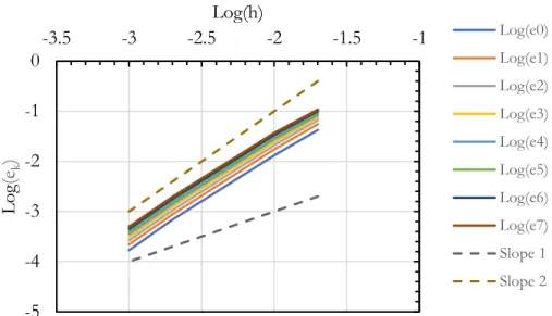
The logarithm of the error is reported as a function of the logarithm of the grid size ℎ = Δ𝑥 in Fig. 2, which illustrates that the second order of accuracy of the advection scheme is recovered for all the moments of the transported moment vector. Numerical values of the errors reported in Fig. 2 are shown in Table 1.
The test case presented in this section serves as preliminary verification of the implementation of the 𝜁 simplified scheme into OpenFOAM. However, the additional limitation of the 𝜁𝑝 quantities was not
triggered while performing the simulations required to produce the results in Fig. 1. Therefore, a different test case was considered to also examine this aspect of the implementation of the scheme, as
0.0 0.2 0.4 0.6 0.8 1.0 0 0.2 0.4 0.6 0.8 1 mk x 0.0 0.2 0.4 0.6 0.8 1.0 0 0.2 0.4 0.6 0.8 1 mk x 0.0 0.2 0.4 0.6 0.8 1.0 0 0.2 0.4 0.6 0.8 1 mk x 0.0 0.2 0.4 0.6 0.8 1.0 0 0.2 0.4 0.6 0.8 1 mk x (a) (b) (c) (d)
Fig. 1: Moments of the regular NDF. Analytical solution (dashed lines) and numerical prediction (solid lines) with (a) 50, (b) 100, (c) 500 and (d) 1000 cells – Zeta scheme.
15
illustrated in Sec. 5.2, where a case involving a multimodal distribution, with moments potentially at the boundary of the moment space is considered.
Table 1: Numerical values of the errors reported in Fig. 2 and corresponding order of the reconstruction of each moment. Cells h e0 Order m0 e1 Order m1 e2 Order m2 e3 Order m3
50 0.02 0.0423 0.0555 0.0665 0.0759
100 0.01 0.0132 1.6851 0.0173 1.6792 0.0210 1.6625 0.0244 1.6359 500 0.002 0.0007 1.8318 0.0009 1.8512 0.0011 1.8509 0.0012 1.8481 1000 0.001 0.0002 2.0240 0.0002 1.9997 0.0003 2.0047 0.0003 2.0055 Cells h e4 Order m4 e5 Order m5 e6 Order m6 e7 Order m7
50 0.02 0.0849 0.0934 0.1013 0.1087
100 0.01 0.0276 1.6187 0.0307 1.6048 0.0337 1.5862 0.0368 1.5614 500 0.002 0.0014 1.8426 0.0016 1.8331 0.0018 1.8235 0.0020 1.8160 1000 0.001 0.0004 2.0023 0.0004 2.0006 0.0004 1.9994 0.0005 1.9851 5.2. One-dimensional advection of moments at the boundary of the moment space
The second test case considers moments of a bimodal NDF, which can be at boundary of the moment space. The initial condition is defined with the help of three weight functions, whose value depends on the position in the computational domain 𝑥 as indicated in Eqs. (5.7) - (5.9).
𝑤1(𝑥) = {16𝑥2(1 − 𝑥)2 0 ≤ 𝑥 ≤ 1 0 otherwise (5.7) -5 -4 -3 -2 -1 0 -3.5 -3 -2.5 -2 -1.5 -1 L og (ek ) Log(h) Log(e0) Log(e1) Log(e2) Log(e3) Log(e4) Log(e5) Log(e6) Log(e7) Slope 1 Slope 2
Fig. 2: Logarithm of the error in the numerical prediction of the moments of the regular NDF case as a function of the logarithm of the grid size – Zeta scheme.
16 𝑤2(𝑥) = { 256 81 (4𝑥 − 1) 2(1 − 𝑥)2 1 4≤ 𝑥 ≤ 1 0 otherwise (5.8) 𝑤3(𝑥) = {9(3𝑥 − 1)2(1 − 𝑥)2 1 3≤ 𝑥 ≤ 1 0 otherwise (5.9) Two other auxiliary functions are introduced as follows:
𝜆2 = { 𝜆2,min= 2 ⋅ 10−2 0 ≤ 𝑥 ≤1 3 𝜆2,min(2 − 3𝑥)2(6𝑥 − 1) + 𝜆max(3𝑥 − 1)2(5 − 6𝑥) 1 3 < 𝑥 ≤ 2 3 𝜆2,max = 0.7 2 3< 𝑥 ≤ 1 , (5.10) 𝜅2 = { 𝜅2,min = 3 0 ≤ 𝑥 ≤ 1 3 𝜅2,min(2 − 3𝑥)2(6𝑥 − 1) + 𝜆max(3𝑥 − 1)2(5 − 6𝑥) 1 3< 𝑥 ≤ 2 3 𝜅2,max = 10 2 3 < 𝑥 ≤ 1 , (5.11)
With these definitions, the value of the initial moments is found according to the expression: 𝑚𝑘(𝑥) = 𝑤1(𝑥)𝑥𝑖,1𝑘 + 𝑤
2(𝑥)(2𝑥𝑖,1) 𝑘
+ 𝑤3(𝑥)𝜆𝑘(𝑥)Γ (1 + 𝑘
𝜅2), (5.12) where 𝑥𝑖,1 = 0.02. The same cases considered in Sec. 5.1 were repeated with the initial condition
17
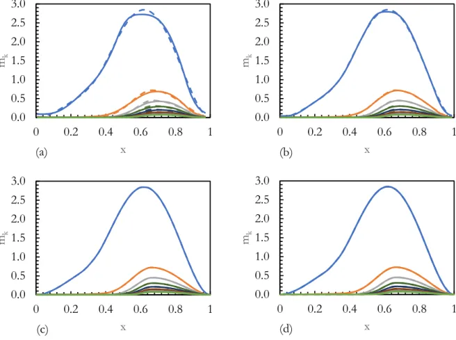
The comparison of the numerical solution and the exact solution is reported in Fig. 3. Similarly, to what is observed in the case of the moments of a regular NDF, also in the case of the moments of the bimodal distribution, the grid resolutions of 50 and 100 cells do not allow to exactly preserve the moments, which are satisfactorily preserved on the grid with 500 and 1000 cells. However, the 𝜁 scheme ensures the realizability of the transported moment vector.
0.0 0.5 1.0 1.5 2.0 2.5 3.0 0 0.2 0.4 0.6 0.8 1 mk x 0.0 0.5 1.0 1.5 2.0 2.5 3.0 0 0.2 0.4 0.6 0.8 1 mk x 0.0 0.5 1.0 1.5 2.0 2.5 3.0 0 0.2 0.4 0.6 0.8 1 mk x 0.0 0.5 1.0 1.5 2.0 2.5 3.0 0 0.2 0.4 0.6 0.8 1 mk x (a) (b) (c) (d)
Fig. 3: Moments of the bimodal NDF. Analytical solution (dashed lines) and numerical prediction (solid lines) with (a) 50, (b) 100, (c) 500 and (d) 1000 cells – Zeta scheme.
18
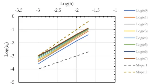
The behavior of the error, defined by Eq. (5.7), in the case of the bimodal NDF is reported in Fig. 4 and the corresponding numerical values are shown in Table 2.
Table 2: Numerical values of the errors reported in Fig. 4 and corresponding order of the reconstruction of each moment. Cells h e0 Order m0 e1 Order m1 e2 Order m2 e3 Order m3
50 0.02 0.0399 0.0731 0.0914 0.1007
100 0.01 0.0137 1.5393 0.0218 1.7427 0.0271 1.7557 0.0304 1.7284 500 0.002 0.0009 1.7199 0.0012 1.7999 0.0013 1.9073 0.0015 1.8837 1000 0.001 0.0002 1.8448 0.0004 1.7585 0.0004 1.6072 0.0005 1.4687 Cells h e4 Order m4 e5 Order m5 e6 Order m6 e7 Order m7
50 0.02 0.1083 0.1165 0.1231 0.1284
100 0.01 0.0339 1.6751 0.0374 1.6374 0.0408 1.5929 0.0439 1.5488 500 0.002 0.0018 1.8360 0.0022 1.7668 0.0026 1.7121 0.0029 1.6885 1000 0.001 0.0007 1.4168 0.0008 1.4466 0.0009 1.4692 0.0011 1.4385
The chart shows that nearly second-order accuracy is achieved for low-order moments. However, the intervention of the additional limiter on the 𝜁 quantities impacts the accuracy of high-order moments. In any case, the order of accuracy of the 𝜁 scheme remains higher than one in all the cases considered in this test, which represents an extreme condition, with moments close to the boundary of the moment space. -5 -4 -3 -2 -1 0 -3.5 -3 -2.5 -2 -1.5 -1 L og(e k ) Log(h) Log(e0) Log(e1) Log(e2) Log(e3) Log(e4) Log(e5) Log(e6) Log(e7) Slope 1 Slope 2
Fig. 4: Logarithm of the error in the numerical prediction of the moments of the bimodal NDF case as a function of the logarithm of the grid size – Zeta scheme.
19
5.3. Two-dimensional advection of moments of a regular NDF
The implementation of the second-order moment-preserving 𝜁 scheme was tested in a two-dimensional case considering a computational domain defined as [0, 0.5] × [0, 0.5], with a steady Taylor-Green velocity field defined as:
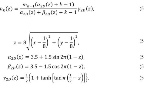
𝐔 = (sin 2𝜋𝑥 cos 2𝜋𝑦 , − cos 2𝜋𝑥 sin 2𝜋𝑦) (5.13) The velocity on cell faces, needed to evaluate the advection flux, was computed by linearly interpolating the velocity field defined in Eq. (5.13) onto the cell faces. The initial value of the moments was defined as follows:
𝑚𝑘(𝑧) = 𝑚𝑘−1(𝛼2𝐷(𝑧) + 𝑘 − 1) 𝛼2𝐷(𝑧) + 𝛽2𝐷(𝑧) + 𝑘 − 1𝛾2𝐷(𝑧), (5.14) where 𝑧 = 8√(𝑥 −1 8) 2 + (𝑦 −1 8) 2 , (5.15) 𝛼2𝐷(𝑧) = 3.5 + 1.5 sin 2𝜋(1 − 𝑧), (5.16) 𝛽2𝐷(𝑧) = 3.5 − 1.5 cos 2𝜋(1 − 𝑧), (5.17) 𝛾2𝐷(𝑧) =12{1 + tanh [tan 𝜋 (1 2− 𝑧)]}. (5.18)
5.3.1. Calculations on quadrilateral grids
The case illustrated in this section was simulated considering five grid resolutions with increasing level of refinement, respectively with 64, 128, 256, 512 in each spatial direction, with a maximum CFL number of 0.2. Results showing the predicted zero-order moment at 𝑡 = 0.8 are shown in Fig. 5.
It is apparent from Fig. 5 that the numerical solution obtained on the two finest grid resolutions with
(a) (b) (c) (d)
Fig. 5: Zero-order moment of the regular NDF used in the two-dimensional test case on quadrilateral grids at t = 0.8. (a) 642 cells, (b) 1282 cells, (c) 2562 cells, (d) 5122 cells. Zeta scheme.
20
2562 and 5122 cells, do not show significant differences. However, to provide a quantitative measure of the accuracy of the zeta scheme, and to validate its implementation into OpenFOAM in comparison
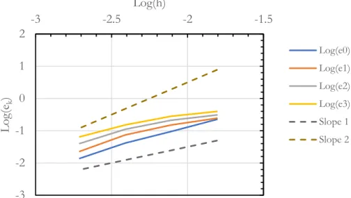
to [1], the order of accuracy of the 𝜁 scheme is quantified numerically by taking the solution obtained on a uniform quadrilateral grid with 10242 cells as reference. The graph of the error is reported in Fig. 6 (numerical values in Table 3), which shows that the slope of the error curves tends to 2 for higher grid resolutions, with a reduction of the formal of order of accuracy for moments of higher order.
Table 3: Numerical values of the errors reported in Fig. 6 and corresponding order of the reconstruction of each moment. Cells h e0 Order m0 e1 Order m1 e2 Order m2 e3 Order m3
64 0.0156 0.2253 0.2451 0.3089 0.3970
128 0.0078 0.0946 1.2527 0.1506 0.7025 0.2115 0.5466 0.2823 0.4921 256 0.0039 0.0419 1.1748 0.0746 1.0130 0.1110 0.9299 0.1531 0.8829 512 0.0020 0.0139 1.5931 0.0229 1.7030 0.0403 1.4637 0.0649 1.2384
The time evolution of the first-order moment of the NDF and of the value of the corresponding limiter 𝜆0,c are reported in Fig. 7.
It is observed that 𝜆0,c = 1 in most of the solution domain. The regions where a complete limitation
is applied (𝜆0,c = 0), reducing the local accuracy to first order, is often where the solution presents
very small positive values of the moment. The additional limitation through 𝜆0,c preserves the
realizability of the moment vector, while showing a limited impact on the accuracy of the solution, as
-3 -2 -1 0 1 2 -3 -2.5 -2 -1.5 L og(e k ) Log(h) Log(e0) Log(e1) Log(e2) Log(e3) Slope 1 Slope 2
Fig. 6: Logarithm of the error in the two-dimensional numerical tests on hexahedral grid with regular NDF as a function of the logarithm of the grid size.
21
previously illustrated by the numerical study of the order of the scheme (Fig. 6).
5.3.2. Calculations on triangular grids
The two-dimensional case presented in this section was also considered to establish the accuracy of the 𝜁 advection scheme on triangular grids. Four grids were considered in these simulations, whose properties are summarized in Table 4. The value of the grid spacing ℎ was calculated according to [72], as ℎ = √𝑁1 𝑐𝑒𝑙𝑙𝑠 ∑(Δ𝐴𝑖) 𝑖 , (5.19)
where Δ𝐴𝑖 is the area of each cell polygon.
Table 4: Properties of the unstructured grids considered in the numerical test cases.
Grid N. of cells Domain area h
A 3938 0.25 7.97 ⋅ 10−3
B 15894 0.25 3.97 ⋅ 10−3
C 64688 0.25 1.97 ⋅ 10−3
D 255596 0.25 9.89 ⋅ 10−4
(a) (b) (c) (d)
Fig. 7: Time evolution of the first-order moment of the regular NDF considered in the test case on quadrilateral grid (resolution shown: 10242): (a) t = 0.2 s; (b) t = 0.4 s; (c) t = 0.6 s; (d) t = 0.8 s.
22
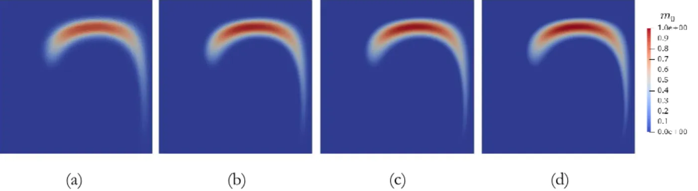
The contour plots of the zero-order moment obtained with the 𝜁 scheme on the triangular grids at 𝑡 = 0.8s, are reported in Fig. 8, which shows the results are visually identical to those obtained on quadrilateral grids and reported in Fig. 5.
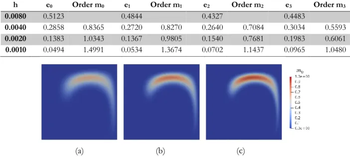
The behavior of the formal order of accuracy of the 𝜁 simplified scheme on triangular grids is shown in Fig. 9 (numerical values in Table 5), which shows comparable trends for all the moments to those observed on quadrilateral grids (Fig. 6), with the second-order accuracy recovered on the finest grids, for the lower-order moments.
5.3.3. Comparison of first-order scheme and 𝜁 simplified scheme
Results obtained with the first-order scheme on a quadrilateral grid are shown in Fig. 10 to highlight
(a) (b) (c) (d)
Fig. 8: Zero-order moment of the regular NDF used in the two-dimensional test case on triangular grids at t = 0.8. (a) Grid A, (b) Grid B, (c) Grid C, (d) Grid D. Zeta scheme.
Fig. 9: Logarithm of the error in the two-dimensional numerical tests on triangular grids with regular NDF as a function of the logarithm of the grid size.
-2 -1 0 1 2 -3.2 -2.7 -2.2 L og(e k ) Log(h) Log(e0) Log(e1) Log(e2) Log(e3) Slope 1 Slope 2
23
the significantly higher dissipation introduced by the first-order scheme, typically used for moment transport to avoid compromising the realizability of the advected moment vector.
Table 5: Numerical values of the errors reported in Fig. 9 and corresponding order of the reconstruction of each moment. h e0 Order m0 e1 Order m1 e2 Order m2 e3 Order m3
0.0080 0.5123 0.4844 0.4327 0.4483
0.0040 0.2858 0.8365 0.2720 0.8270 0.2640 0.7084 0.3034 0.5593 0.0020 0.1383 1.0343 0.1367 0.9805 0.1540 0.7681 0.1983 0.6061 0.0010 0.0494 1.4991 0.0534 1.3674 0.0702 1.1437 0.0965 1.0480
The difference between the first-order scheme and the second-order zeta scheme is further highlighted in Fig. 11, where the zero-order moment obtained at 𝑡 = 0.8s on a grid with 1282 cells with the two methods is compared. The results obtained with the 𝜁 simplified scheme clearly shows the reduced dissipation compared to the results obtained with the first-order scheme.
(a) (b) (c)
Fig. 10: Zero-order moment field at t = 0.8 on a quadrilateral grid with (a) 1282, (b) 2562 and (c) 5122 cells – First-order scheme.
(a) (b)
Fig. 11: Comparison of zero-order moment field obtained on a 1282 quadrilateral grid at t = 0.8, with (a) first-order advection scheme and (b) zeta scheme.
24
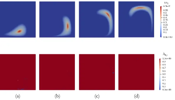
Similarly to what done for the quadrilateral case, the time evolution of the first-order moment of the NDF is shown in Fig. 12, where the fields of 𝑚1 at different times appear to be identical to those
shown in Fig. 7 for the quadrilateral case. However, a more careful examination of the behavior of the moment limiter 𝜆0,c shows that the region of the computational domain where the limitation is
applied is larger for the case with triangular grid compared to the quadrilateral case. Several cells on the front of the region where 𝑚1 ≠ 0 are affected by the limitation, while, in the quadrilateral case, a
smaller number of cells with 𝜆0,c ≠ 1 is observed. The last snapshot (Fig. 12(d)) also shows a small
number of cells where 𝜆0,c= 0.5.
5.4. Two-dimensional advection of moments of a bimodal NDF
The 𝜁 simplified scheme is applied in this section to the case transport of moments of a bi-modal NDF in two dimensions. Only one triangular grid (Grid B in Table 4) is considered.
The initial conditions for the moments are obtained using Eq. (5.12), where the 𝑥 coordinate is replaced by
(a) (b) (c) (d)
Fig. 12: Time evolution of the first-order moment of the regular NDF in the test case on tetrahedral grid (Grid B) and the corresponding limiter 𝜆0,𝑐 used in the additional limitation of the 𝜁 simplified scheme. (a) t = 0.2 s; (b) t = 0.4 s; (c) t = 0.6 s; (d) t = 0.8 s.
25 𝑧 = 8√(𝑥 −1 8) 2 + (𝑦 −1 8) 2 . (5.20)
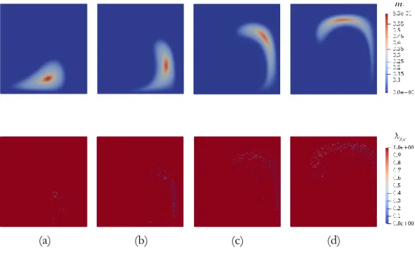
Fig. 13 shows the time evolution of 𝑚0 and 𝑚1 together with the limiter 𝜆0,c used in the additional
limitation in the 𝜁 simplified scheme for the reconstruction of 𝑚1. The figure shows that to preserve
the moment realizability, the additional limitation intervenes in a modest number of cells, as expected because of the moment vectors near the boundary of the moment space.
Finally, it should be noted that the limitation applied to the second-order moment happens in some additional cells, compared to what shown in Fig. 13. This is shown, for example, in Fig. 14 (b), which shows the second-order moment for the case of the bimodal NDF and the corresponding value of the limiter 𝜆1,𝑐 used in the 𝜁 simplified scheme. The limiter is similarly applied to the third-order
moment.
(a) (b) (c) (d)
Fig. 13: Time evolution of the first-order moment of the bi-modal NDF in the test case on tetrahedral grid (Grid B) and the corresponding limiter
𝜆0,𝑐used in the additional limitation of the ζ simplified scheme. (a) t = 0.2
26
6. Conclusions
The second-order realizable 𝜁 simplified scheme proposed in Laurent and Nguyen [1] was extended to unstructured grids and implemented into the computational framework OpenQBMM [73], an extension for OpenFOAM [63] that implements quadrature-based moment methods. The implementation was verified by considering first two one-dimensional cases, the first involving moments of a regular NDF and the second where moments of a bimodal NDF are transported. The proposed implementation of the scheme into OpenQBMM was able to reproduce the results for the same cases reported in Laurent and Nguyen [1], showing convergence to second-order accuracy with grid refinement. The scheme was further verified on a two-dimensional case with uniform hexahedral discretization where the first four moments of a regular NDF are transported. Also in this case, results from Laurent and Nguyen [1] were satisfactorily reproduced. Finally, the same two-dimensional case considered for verification on hexahedral grids was used to establish the accuracy of the scheme on triangular grids. The 𝜁 simplified scheme was able to reproduce the results and the behavior of the error affecting the solution observed on hexahedral grids also on triangular grids. Future work will consider the development of realizable numerical schemes for multivariate problems, where closure is provided by the conditional quadrature method of moments [74].
7. Source code and test cases
The source code of the OpenQBMM framework [73] used to perform the calculations described in
Fig. 14: (a) Second-order moment of the bi-modal NDF in the test case on tetrahedral grid (Grid B) at t = 0.8, and, (b), the corresponding field of the limiter 𝜆1,𝑐 used in the additional
limitation of the ζ simplified scheme.
27
this article is available in [73,75], where also the test cases presented in the articles are available. The OpenFOAM class implementing the 𝜁 scheme on unstructured grids described in the manuscript is reported in Appedix A.
8. Acknowledgements
The authors would like to gratefully acknowledge the support of the US National Science Foundation under the SI2–SSE award NSF–ACI 1440443 and the support of the French National Research Agency (ANR) under grant ANR-13-TDMO-02 ASMAPE for the ASMAPE project.
A.P. would like to acknowledge the support of the Jean d’Alembert fellowship program Idex Saclay, which supported his stay at Laboratoire EM2C, CNRS, CentraleSupélec, Université Paris-Saclay.
Appedix A
The C++ source code of the main class that implements the 𝜁 scheme in OpenQBMM is reported in this appendix. This code is contained in OpenQBMM 5.0.0 for OpenFOAM 7 [75].
Header file: zetaUnivariateAdvection.H
/*---*\ ========= |
\\ / F ield | OpenFOAM: The Open Source CFD Toolbox \\ / O peration |
\\ / A nd | Copyright (C) 2014-2018 Alberto Passalacqua \\/ M anipulation |
---License
This file is derivative work of OpenFOAM.
OpenFOAM is free software: you can redistribute it and/or modify it under the terms of the GNU General Public License as published by the Free Software Foundation, either version 3 of the License, or (at your option) any later version.
OpenFOAM is distributed in the hope that it will be useful, but WITHOUT ANY WARRANTY; without even the implied warranty of MERCHANTABILITY or FITNESS FOR A PARTICULAR PURPOSE. See the GNU General Public License for more details.
You should have received a copy of the GNU General Public License along with OpenFOAM. If not, see <http://www.gnu.org/licenses/>. Class
28 Foam::zeta
Description
Second-order univariate moment advection with zeta kinetic scheme. SourceFiles zetaUnivariateAdvection.C \*---*/ #ifndef zetaUnivariateAdvection_H #define zetaUnivariateAdvection_H #include "univariateMomentAdvection.H" // * * * * * * * * * * * * * * * * * * * * * * * * * * * * * * * * * * * * // namespace Foam { namespace univariateAdvection { /*---*\ Class zeta Declaration
\*---*/ class zeta : public univariateMomentAdvection { // Private data
//- Reference to zero-order moment field
const volScalarField& m0_; //- Reconstructed m0 (owner) surfaceScalarField m0Own_; //- Reconstructed m0 (neighbour) surfaceScalarField m0Nei_;
//- Number of zeta_k values
label nZetas_;
//- List of fields of zeta_k (n fields for n + 1 moments)
PtrList<volScalarField> zetas_;
//- List of interpolated zeta_k values (neighbour)
PtrList<surfaceScalarField> zetasNei_;
//- List of interpolated nodes (owner)
PtrList<surfaceScalarField> zetasOwn_;
//- List of interpolated zeta_k values (neighbour)
PtrList<surfaceScalarField> zetasUpwindNei_;
29 //- List of interpolated nodes (owner)
PtrList<surfaceScalarField> zetasUpwindOwn_;
//- List of interpolated zeta_k values (neighbour)
PtrList<surfaceScalarField> zetasCorrNei_;
//- List of interpolated nodes (owner)
PtrList<surfaceScalarField> zetasCorrOwn_;
//- List of interpolated moments (neighbour)
PtrList<surfaceScalarField> momentsNei_;
//- List of interpolated moments (owner)
PtrList<surfaceScalarField> momentsOwn_;
//- Field to store the number of faces with outgoing flux per cell
mutable labelField nFacesOutgoingFlux_;
//- Field to store the number of realizable moments in each cell
mutable labelField nRealizableMoments_;
//- Field to store the number of realizable m* in each cell
mutable labelField nRealizableMomentsStar_;
//- List of limiters for zeta_k
PtrList<surfaceScalarField> limiters_;
//- List of cell limiters
PtrList<volScalarField> cellLimiters_;
//- Face velocity
const surfaceScalarField& phi_;
// Private member functions
//- Compute n values of zeta_k from n + 1 moments
void computeZetaFields();
//- Updates reconstructed moments from the values of zeta
void updateMomentFieldsFromZetas (
const surfaceScalarField& m0f,
const PtrList<surfaceScalarField>& zetaf, PtrList<surfaceScalarField>& mf
);
//- Compute n + 1 moments from n values of zeta_k
void zetaToMoments (
const scalarList& zetaf, scalarList& mf, scalar m0 = 1.0 ); protected:
30
// Protected member functions
//- Calculates the number of cells with outgoing flux
void countFacesWithOutgoingFlux();
//- Computes the limiter used for additional limitation
void limiter();
//- Reconstructs zeta_k
void interpolateFields();
//- Applies additional limitation to zeta_k, if needed
void limitZetas();
public:
//- Runtime type information
TypeName("zeta");
// Constructors
//- Construct from univariateMomentSet
zeta (
const dictionary& dict,
const scalarQuadratureApproximation& quadrature, const surfaceScalarField& phi,
const word& support ); //- Destructor virtual ~zeta();
// Public member functions
//- Return the maximum Courant number ensuring moment realizability
virtual scalar realizableCo() const;
//- Update moment advection
virtual void update(); }; // * * * * * * * * * * * * * * * * * * * * * * * * * * * * * * * * * * * * * //
} // End namespace univariateAdvection
} // End namespace Foam
// * * * * * * * * * * * * * * * * * * * * * * * * * * * * * * * * * * * * * //
31 // * * * * * * * * * * * * * * * * * * * * * * * * * * * * * * * * * * * * * // #endif // ************************************************************************* //
Class implementation: zetaUnivariateAdvection.C
/*---*\ ========= |
\\ / F ield | OpenFOAM: The Open Source CFD Toolbox \\ / O peration |
\\ / A nd | Copyright (C) 2014-2018 Alberto Passalacqua \\/ M anipulation |
---License
This file is derivative work of OpenFOAM.
OpenFOAM is free software: you can redistribute it and/or modify it under the terms of the GNU General Public License as published by the Free Software Foundation, either version 3 of the License, or (at your option) any later version.
OpenFOAM is distributed in the hope that it will be useful, but WITHOUT ANY WARRANTY; without even the implied warranty of MERCHANTABILITY or FITNESS FOR A PARTICULAR PURPOSE. See the GNU General Public License for more details.
You should have received a copy of the GNU General Public License along with OpenFOAM. If not, see <http://www.gnu.org/licenses/>.
\*---*/ #include "zetaUnivariateAdvection.H" #include "upwind.H" #include "addToRunTimeSelectionTable.H"
// * * * * * * * * * * * * * * Static Data Members * * * * * * * * * * * * //
namespace Foam { namespace univariateAdvection { defineTypeNameAndDebug(zeta, 0); addToRunTimeSelectionTable ( univariateMomentAdvection, zeta, dictionary );
32 } } // * * * * * * * * * * * * * * * * Constructors * * * * * * * * * * * * * //
Foam::univariateAdvection::zeta::zeta (
const dictionary& dict,
const scalarQuadratureApproximation& quadrature,
const surfaceScalarField& phi,
const word& support
) :
univariateMomentAdvection(dict, quadrature, phi, support), m0_(moments_(0)),
m0Own_ (
IOobject::groupName("m0OwnZeta", name_),
fvc::interpolate(m0_, own_, "reconstruct(m0)") ),
m0Nei_ (
IOobject::groupName("m0NeiZeta", name_),
fvc::interpolate(m0_, nei_, "reconstruct(m0)") ), nZetas_(nMoments_ - 1), zetas_(nZetas_), zetasNei_(nZetas_), zetasOwn_(nZetas_), zetasUpwindNei_(nZetas_), zetasUpwindOwn_(nZetas_), zetasCorrNei_(nZetas_), zetasCorrOwn_(nZetas_), momentsNei_(nMoments_), momentsOwn_(nMoments_), nFacesOutgoingFlux_(m0_.size(), 0), nRealizableMoments_(m0_.size(), 0), nRealizableMomentsStar_(m0_.size(), 0), limiters_(nZetas_), cellLimiters_(nZetas_), phi_(phi) {
if (quadrature.momentOrders()[0].size() > 1) {
FatalErrorInFunction
<< "Zeta advection scheme can only be used for" << nl << "univariate distributions."
<< abort(FatalError); }
// Populating zeta_k fields and interpolated zeta_k fields
forAll(zetas_, zetai) { zetas_.set ( zetai, new volScalarField (
33 IOobject
(
fieldName("zeta", {zetai}), phi.mesh().time().timeName(), phi.mesh(),
IOobject::NO_READ, IOobject::AUTO_WRITE ),
phi.mesh(),
dimensionedScalar("zero", dimless, 0.0) ) ); zetasNei_.set ( zetai, new surfaceScalarField ( IOobject (
fieldName("zetaNei", {zetai}), phi.mesh().time().timeName(), phi.mesh(),
IOobject::NO_READ, IOobject::NO_WRITE ),
phi.mesh(),
dimensionedScalar("zero", dimless, 0.0) ) ); zetasOwn_.set ( zetai, new surfaceScalarField ( IOobject (
fieldName("zetaOwn", {zetai}), phi.mesh().time().timeName(), phi.mesh(),
IOobject::NO_READ, IOobject::NO_WRITE ),
phi.mesh(),
dimensionedScalar("zero", dimless, 0.0) ) ); zetasUpwindNei_.set ( zetai, new surfaceScalarField ( IOobject (
34
phi.mesh().time().timeName(), phi.mesh(),
IOobject::NO_READ, IOobject::NO_WRITE ),
phi.mesh(),
dimensionedScalar("zero", dimless, 0.0) ) ); zetasUpwindOwn_.set ( zetai, new surfaceScalarField ( IOobject (
fieldName("zetaUpwindOwn", {zetai}), phi.mesh().time().timeName(),
phi.mesh(),
IOobject::NO_READ, IOobject::NO_WRITE ),
phi.mesh(),
dimensionedScalar("zero", dimless, 0.0) ) ); zetasCorrNei_.set ( zetai, new surfaceScalarField ( IOobject (
fieldName("zetaCorrNei", {zetai}), phi.mesh().time().timeName(), phi.mesh(),
IOobject::NO_READ, IOobject::NO_WRITE ),
phi.mesh(),
dimensionedScalar("zero", dimless, 0.0) ) ); zetasCorrOwn_.set ( zetai, new surfaceScalarField ( IOobject (
fieldName("zetaCorrOwn", {zetai}), phi.mesh().time().timeName(), phi.mesh(),
35 IOobject::NO_WRITE ),
phi.mesh(),
dimensionedScalar("zero", dimless, 0.0) ) ); limiters_.set ( zetai, new surfaceScalarField ( IOobject (
fieldName("zetaLimiter", {zetai}), phi.mesh().time().timeName(), phi.mesh(),
IOobject::NO_READ, IOobject::NO_WRITE ),
phi.mesh(),
dimensionedScalar("zero", dimless, 1.0) ) ); cellLimiters_.set ( zetai, new volScalarField ( IOobject (
fieldName("zetaCellLimiter", {zetai}), phi.mesh().time().timeName(),
phi.mesh(),
IOobject::NO_READ, IOobject::NO_WRITE ),
phi.mesh(),
dimensionedScalar("zero", dimless, 1.0) )
); }
// Setting face values of moments
forAll(momentsNei_, momenti) { momentsNei_.set ( momenti, new surfaceScalarField (
fieldName("momentNeiZeta", {momenti}), fvc::interpolate(moments_(momenti)) )
);
36 momentsOwn_.set ( momenti, new surfaceScalarField (
fieldName("momentOwnZeta", {momenti}), fvc::interpolate(moments_(momenti)) ) ); } } // * * * * * * * * * * * * * * * * Destructor * * * * * * * * * * * * * * //
Foam::univariateAdvection::zeta::~zeta() {}
// * * * * * * * * * * * * * * * Member Functions * * * * * * * * * * * * //
void Foam::univariateAdvection::zeta::interpolateFields() {
IStringStream m0OwnLimiter("Minmod"); IStringStream zetaOwnLimiter("Minmod");
tmp<surfaceInterpolationScheme<scalar>> m0OwnScheme (
fvc::scheme<scalar>(own_, m0OwnLimiter) );
tmp<surfaceInterpolationScheme<scalar>> zetaOwnScheme (
fvc::scheme<scalar>(own_, zetaOwnLimiter) );
IStringStream m0NeiLimiter("Minmod"); IStringStream zetaNeiLimiter("Minmod");
tmp<surfaceInterpolationScheme<scalar>> m0NeiScheme (
fvc::scheme<scalar>(nei_, m0NeiLimiter) );
tmp<surfaceInterpolationScheme<scalar>> zetaNeiScheme (
fvc::scheme<scalar>(nei_, zetaNeiLimiter) );
m0Own_ = m0OwnScheme().interpolate(moments_(0)); m0Nei_ = m0NeiScheme().interpolate(moments_(0));
forAll(zetas_, zetai) {
zetasNei_[zetai] = zetaNeiScheme().interpolate(zetas_[zetai]); zetasOwn_[zetai] = zetaOwnScheme().interpolate(zetas_[zetai]);
zetasUpwindNei_[zetai] =
37
zetasUpwindOwn_[zetai] =
upwind<scalar>(zetas_[zetai].mesh(), own_).flux(zetas_[zetai]);
zetasCorrNei_[zetai] = zetasNei_[zetai] - zetasUpwindNei_[zetai]; zetasCorrOwn_[zetai] = zetasOwn_[zetai] - zetasUpwindOwn_[zetai]; }
}
void Foam::univariateAdvection::zeta::zetaToMoments (
const scalarList& zetaf,
scalarList& mf, scalar m0 ) { scalarSquareMatrix S(nMoments_, 0.0);
for (label i = 0; i < nZetas_; i++) {
S[0][i] = 1.0; }
for (label i = 1; i < nZetas_; i++) {
for (label j = i; j < nZetas_; j++) {
S[i][j] = S[i][j - 1] + zetaf[j - i]*S[i - 1][j]; }
}
scalarList prod(nMoments_, 1.0);
prod[1] = zetaf[0];
for (label i = 2; i < nZetas_; i++) {
prod[i] = prod[i - 1]*zetaf[i - 1]; }
// Resetting moments to zero
mf = 0.0; // Computing moments mf[0] = 1.0; mf[1] = zetaf[0];
for (label i = 2; i < nMoments_; i++) { for (label j = 0; j <= i/2; j++) { mf[i] += prod[i - 2*j]*sqr(S[j][i - j]); } } if (m0 != 1.0) {
38
for (label mi = 0; mi < nMoments_; mi++) { mf[mi] *= m0; } } }
void Foam::univariateAdvection::zeta::computeZetaFields() { // Cell-center values forAll(m0_, celli) { if (m0_[celli] >= SMALL) {
univariateMomentSet m(nMoments_, support_);
for (label mi = 0; mi < nMoments_; mi++) {
m[mi] = moments_(mi)[celli]; }
nRealizableMoments_[celli] = m.nRealizableMoments();
scalarList zetas(m.zetas());
for (label zetai = 0; zetai < nZetas_; zetai++) {
zetas_[zetai][celli] = zetas[zetai];
if (zetas_[zetai][celli] > 1.0e-7) {
zetas_[zetai][celli] = zetas[zetai]; }
else
{
zetas_[zetai][celli] = 0.0; } } } } // Boundary conditions
const volScalarField::Boundary& bf = zetas_[0].boundaryField();
forAll(bf, patchi) {
const fvPatchScalarField& m0Patch = bf[patchi];
forAll(m0Patch, facei) {
if (m0_.boundaryField()[patchi][facei] >= SMALL) {
univariateMomentSet m(nMoments_, support_);
for (label mi = 0; mi < nMoments_; mi++) {
39 }
scalarList zetas(m.zetas());
for (label zetai = 0; zetai < nZetas_; zetai++) {
volScalarField& zi = zetas_[zetai];
volScalarField::Boundary& ziBf = zi.boundaryFieldRef(); ziBf[patchi][facei] = zetas[zetai];
} } } } }
void Foam::univariateAdvection::zeta::countFacesWithOutgoingFlux() {
const fvMesh& mesh(phi_.mesh());
const labelList& own = mesh.faceOwner();
const labelList& nei = mesh.faceNeighbour();
nFacesOutgoingFlux_ = 0;
// Counting internal faces with outgoing flux
for (label facei = 0; facei < mesh.nInternalFaces(); facei++) {
if (phi_[facei] > 0) {
nFacesOutgoingFlux_[own[facei]] += 1; }
else if (phi_[facei] < 0) {
nFacesOutgoingFlux_[nei[facei]] += 1; }
}
// Adding boundary faces with outgoing flux
const surfaceScalarField::Boundary& phiBf = phi_.boundaryField();
forAll(phiBf, patchi) {
const fvsPatchScalarField& phiPf = phiBf[patchi];
const labelList& pFaceCells = mesh.boundary()[patchi].faceCells();
forAll(phiPf, pFacei) {
if (phiPf[pFacei] > 0) {
nFacesOutgoingFlux_[pFaceCells[pFacei]] += 1; }
} } }
void Foam::univariateAdvection::zeta::limitZetas() {