HAL Id: hal-03004383
https://hal.archives-ouvertes.fr/hal-03004383
Preprint submitted on 13 Nov 2020
HAL is a multi-disciplinary open access archive for the deposit and dissemination of sci-entific research documents, whether they are pub-lished or not. The documents may come from teaching and research institutions in France or abroad, or from public or private research centers.
L’archive ouverte pluridisciplinaire HAL, est destinée au dépôt et à la diffusion de documents scientifiques de niveau recherche, publiés ou non, émanant des établissements d’enseignement et de recherche français ou étrangers, des laboratoires publics ou privés.
Firm growth in developing countries: Driven by external
shocks or internal characteristics?
Florian Léon
To cite this version:
Florian Léon. Firm growth in developing countries: Driven by external shocks or internal character-istics?. 2020. �hal-03004383�
fondation pour les études et recherches sur le développement international ATION REC ONNUE D ’UTILITÉ PUBLIQUE . VEC L ’IDDRI L ’INITIA TIVE POUR LE DÉ VEL OPPEMENT E
T LA GOUVERNANCE MONDIALE (IDGM).
’ASSOCIE A U CERDI E T À L ’IDDRI. ATION A BÉNÉFICIÉ D ’UNE AIDE DE L ’É TA T FR ANC AIS GÉRÉE P AR L ’ANR A U TITRE DU PR OGR A MME «INVESTISSEMENT S D ’A VENIR» -14-01». Abstract
The purpose of this paper is to assess the importance of external shocks relative to internal characteristics in explaining variation of firm growth in developing countries. To do so, we compile firm-level panel data covering 12,562 firms operating in 72 low-income and middle-income countries. Our statistical analysis reveals that, on average, firm characteristics account for a half of difference in growth rate across firms. However, the importance of internal factors is halved when we exclude firms in the tails of the distribution (top performers and worst performers). On the other hand, external shocks account for less than one tenth of variance. The role of external shocks is, however, stronger for young firms and for firms operating in unstable environments. Finally, our findings suggest that the external context is more crucial for exit than for growth.
Keywords: Firm growth; Developing countries; Firm characteristics: External shocks
Firm growth in
developing countries:
Driven by external shocks
or internal characteristics?
Florian Léon
Florian Léon, Research Officer, FERDI. Email: [email protected]
De
velop
ment P
oli
cie
s
Wo
rking
Paper
1
Introduction
The need to create sustainable jobs is an urgent need worldwide, especially in many developing countries due to demographic challenge ahead. Because they provide stable jobs, the development of formal firms is of prime interest for policymakers and academics. In the absence of formal jobs, a majority of young people in developing countries is con-fronted with unsatisfied alternatives such as creation of subsistence activities or migration. Firms in developing countries are often informal and consist of single-worker activities. Formal enteprises are not only less numbered but also smaller than those operating in
industrialized countries (Hsieh and Olken, 2014). A few firms are able to grow over the
life-cycle (Hsieh and Klenow, 2014; Eslava et al., 2019). Large firms are often large at
birth (Ayyagari et al.,2020).
Many efforts have therefore been devoted to understand and tackle obstacles to (small) firm growth in developing world. A first generation of works has highlighted the impor-tance of the institutional context in which firms operate to explain difference in growth rates. These works investigate the impact of financial development (Beck and
Demirguc-Kunt, 2006), fiscal and regulatory framework (Klapper et al., 2006), corruption (Fisman
and Svensson, 2007) or the lack of instractructures (Cole et al., 2018). A new body of
research, which will gain interest with the recent Covid-crisis, has concentrated on the im-pact of external shocks (commodity price booms and busts, natural disasters, epidemics
or civil conflict) on the dynamics of firms in developing countries (Bowles et al., 2016;
Elliott et al.,2019;Dosso and L´eon, 2020).
Another strand of literature has focused on firm-level attributes. Premilinary works have focused on observable structural characteristics of the firm (size, age or sector) or
of the entrepreneur (education, experience) to explain performance of firms (see Nichter
and Goldmark,2009;Woodruff,2018). In the footsteps ofBloom and Van Reenen(2007),
recent articles have considered the internal organization of the firm. These papers focus on the impact of (changes in) managerial practices as a strong determinant of firm
per-formance (Bloom et al.,2013;McKenzie and Woodruff, 2016). This approach dedicating
a special attention to firm-level attributes is in line with a rich literature in managerial
(the resource-based view and evolutionary economics) assume that growing firms have specific resources or attributes that permit them to outperform their competitors.
The aim of this paper is to adopt a new perspective by assessing the relative
impor-tance of internal (firm) characteristics versus external factors1 in explaining variation of
employment growth in developing world. Rather than focusing on a specific (internal or external) factor, we measure the explanatory power of both strands of explanations. To do so, we exploit the World Bank Enterprise Surveys. We follow a panel of 12,562 firms operating in 72 developing countries over the period 2006-2018. We decompose the total variance of firm growth between explained variable (by the model) and unexplained variance (residual variance). We consider models including internal and external factors separately and then jointly. For internal factors, we consider in addition to structural characteristics of the firm (size, age, ownership), firm fixed effects allowing us to account for (unobserved) time-invariant characteristics (such as entrepreneur structural charac-teristics or weakly time-varying internal organization). For contextual factors, we assess the importance of sectoral and local shocks, irrespective of their origin. To do so, we add sector-country-time dummies that account for sectoral shocks occurring in one country in one period and (sub-national) location-time dummies taking into account local shocks. To briefly summarize our results, we show that firm-level factors explain the largest share of variance of firm growth. Approximatively one half of variance is explained by firm characteristics. At the opposite, external shocks account, on average, for less than 10% of total variance. In detail, we document that the role of internal factors is predominant for leaders (best performers in the long-run) and losers (worst performers). When we exclude leaders and losers the contribution of internal factors is halved. In addition, the role played by local and sectoral shocks is stronger for young firms (below 10-year old) and for firms operating in unstable environments. However, we fail to detect a real difference between firms according to their size. Finally, we suggest that external factors play a stronger role in explaining exit than growth. However, this finding is just suggestive insofar as models for exit and growth are not directly comparable.
Our article contributes to the literature on firm dynamics in developing countries. 1Throughout the paper, we interchangeably employ firm characteristics and internal factors on the one hand; and, on the other hand contextual factors and external factors.
Recent works have shown that firm dynamics is weakly explained by within-firm growth
in developing countries (Hsieh and Klenow, 2014; Eslava et al., 2019; Ayyagari et al.,
2017, 2020). This paper adds to this literature by examining the relative importance of
internal and external factors in explaining differences in within-firm growth. In doing so, we employ a data-driven methodology to study the weight of each explanation.
Clos-est to our paper is Ayyagari et al. (2020). The authors document that size at birth is
crucial to explain variation in firm size and growth over the life cycle, contrary to insti-tutional factors. Our work complements this article by adopting an alternative, albeit
complementary, perspective. Contrary to Ayyagari et al. (2020) we are not interested
by specific firm- or country-level characteristics but rather by the explanatory power of internal versus external factors, irrespective of their sources. In addition, we focus not only on institutional characteristics but also on shocks occuring within a country at a local or sectoral level. Finally, we are able to follow closely the evolution of entreprises, rather than exploiting only initial and final observations. In this respect, our work is
more closely related toAyyagari et al. (2017) andEslava et al. (2019), which follow new
ventures in India and Colombia to characterize their life-cycle dynamics. We cannot track firms each year but our sample includes a large number of emerging and developing countries. In this way, we propose a new way to exploit the panel version of the WBESs.
This article also resounds with macroeconomic debate about growth. Economic
growth is highly unstable in developing countries (Easterly et al., 1993; Rodrik, 1999;
Pritchett, 2000). While growth accelerations are frequent, they rarely persist over time
and are highly unpredictable (Hausmann et al., 2005). Microeconomic evidence points
out that the same process also occurs at the firm-level (see L´eon, 2020, for a review).
Our work offers a new perspective by directly scrutinizing the impact of shocks on firm growth. Our statistical analysis documents that external shocks have a limited power, on average, to explain differences in firm growth. Nonetheless, these shocks have a stronger effect on small firms and for firms operating in highly unstable countries.
The paper proceeds as follows. Section 2 presents the data and variables. Section 3
discusses the methodology. Section 4 presents baseline results and extensions. The last
2
Data and variables
2.1
Data
We rely on the most comprehensive firm-level survey data; the World Bank Enterprise Surveys (WBES). In an ideal set-up, we would employ administrative data or census. However, these datasets are rarely available in many developing countries and are not
always comparable across countries.2 The WBES are collected in face-to-face interviews
with top managers and business owners and cover a large range of topics. While the survey is not mandatory, WBES are plant-level surveys of a representative sample of an economy’s formal private sector.
Recently, the WBES’ staff has built a panel by interviewing the same firm during different waves. We therefore consider all firms with at least two observations (two waves) to be able to track firm growth over time. This rule creates a survivorship bias. First, in some countries, there is no panel version of the WBES. Second, when interviewers try to recontact firms surveyed in a previous wave, they sometimes fail because firms were inactive in the second wave or because they were not surveyed for another reason (refuse to answer, impossible to contact them, etc.). These firms are therefore dropped in the analysis. Fortunately, the WBES give information about why a firm was not re-interviewed in the second wave. We present evidence in the following indicating that our findings are not driven by a survivorship bias.
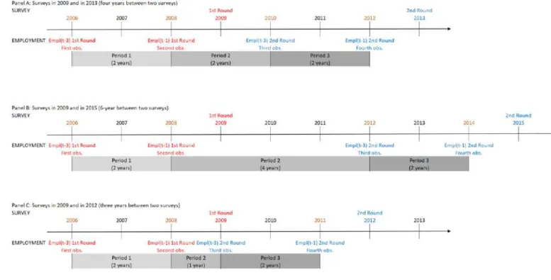
After compiling firms with at least two surveys, we transform data to construct firm growth at different periods. For each wave, we know the number of employees in the past year and three years before the survey. These variables allows us to compute three periods of growth for each firm surveyed twice. To describe the procedure, we take the
example of a firm surveyed in 2009 and in 2013, as shown in Panel A of Figure 1. For
this firm, we know the number of employees for four different years: 2006, 2008, 2010 and 2012. Indeed, we get information on employment in the year before the surveys (i.e., 2008 2Data on firms can be extracted from three different sources: administrative data, census and surveys. Administrative data covers the universe of (formal) firms and are often updated regularly (each year). They provides basic information such as date of creation/exit, location, number of workers. Sometimes, they can also include basic financial figures (assets, sales, profit). Census are between administrative data and surveys. They are implemented less frequently than administrative data and do not cover the universe of firms. However, their participation is mandatory.
and 2012) but also three years before for each survey (i.e., in 2006 for the first survey and in 2010 for the second survey). Based on these four values, we are able to compute job growth for three different periods (of two years each): 2006-08; 2008-10; and 2010-12.
Figure 1: Description of period calculation
The previous example of two surveys separated by four years is not only the most simple (because we get three 2-year periods) but it is also the most frequent, as indicated
in Table1. Indeed, 45% of surveys are separated by four years. In Figure1, we investigate
two alternative possibilities. In Panel B, we consider two surveys separated by six years (e.g., Malawi) and in Panel C two surveys separated by three years (e.g., Russia). The former situation occurs frequently. The time lapse between two surveys in the same
country is of 5 years in 12% of surveys and 6 or 7 years in 19% of surveys (cf. Table 1).
The latter situation is less frequent (only 8% of surveys were separated by three years).3
The first period and third period are unchanged (2-year). Only the second period is affected by the time lapse between surveys because it exploits information from two 3We exclude Myanmar because two surveys were implemented with only two years between them (2014 and 2016).
different surveys as indicated in Figure 1. We discuss the sensitivity of our econometric results to this point in the robustness checks.
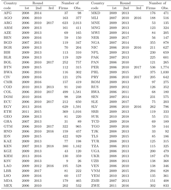
Table 1: Sample of firms per country
Country Round Number of Country Round Number of
code 1st 2nd 3rd Firms Obs. code 1st 2nd 3rd Firms Obs.
AFG 2008 2014 37 98 MKD 2009 2013 176 471 AGO 2006 2010 163 377 MLI 2007 2010 2016 188 516 ARG 2006 2010 2017 623 2,013 MNE 2009 2013 53 135 ARM 2009 2013 161 411 MNG 2009 2013 123 324 AZE 2009 2013 69 165 MWI 2009 2014 84 205 BEN 2009 2016 59 150 NER 2009 2017 56 147 BGD 2007 2013 119 347 NGA 2007 2014 355 878 BGR 2009 2013 70 204 NIC 2006 2010 2016 211 627 BIH 2009 2013 113 310 NPL 2009 2013 230 659 BLR 2008 2013 119 329 PAK 2007 2013 225 601 BOL 2006 2010 2017 252 757 PAN 2006 2010 121 265 BTN 2009 2015 112 315 PER 2006 2010 2017 536 1,774 BWA 2006 2010 116 302 PHL 2009 2015 375 1,030 CIV 2009 2016 121 276 PRY 2006 2010 2017 205 642 CMR 2009 2016 157 419 ROM 2009 2013 97 275 COD 2010 2013 2013 91 240 RUS 2009 2012 126 352 COL 2006 2010 2017 499 1,581 RWA 2006 2011 68 180 DOM 2010 2016 98 238 SEN 2007 2014 231 575 ECU 2006 2010 2017 212 650 SLE 2009 2017 75 203 EGY 2013 2016 629 1,591 SLV 2006 2010 2016 262 796 ETH 2011 2015 369 1,016 SRB 2009 2013 119 333 GEO 2008 2013 81 220 SUR 2010 2018 55 151 GHA 2007 2013 31 89 TCD 2009 2018 69 189 GTM 2006 2010 2017 322 965 TGO 2009 2016 59 144 HND 2006 2010 2016 159 457 TJK 2008 2013 33 92 IDN 2009 2015 422 929 TLS 2009 2015 85 186 KAZ 2009 2013 77 198 TUR 2008 2013 125 315 KEN 2007 2013 2018 380 1,162 TZA 2006 2013 115 325 KGZ 2009 2013 43 120 UGA 2006 2013 200 479 KHM 2013 2016 130 359 UKR 2008 2013 187 470 KSV 2009 2013 9 26 UZB 2008 2013 138 368 LAO 2009 2012 2016 195 528 VEN 2006 2010 138 346 LBR 2009 2017 81 222 VNM 2009 2015 294 828 LSO 2009 2016 60 157 YEM 2010 2013 135 361 MDA 2009 2013 179 465 ZMB 2007 2013 151 408 MEX 2006 2010 202 532 ZWE 2011 2016 302 833
Data were retrieved in October 2019. We consider all firms include in the panel version of the WBES (i.e., re-interviewed firms). Nonetheless, we exclude observations when the interviewer did not believe that answers were trustful (question a16 ). The final sample includes 12,562 firms (34,701 observations) operating in 72 low-income and middle-income
2.2
Variables
2.2.1 Firm growth
Although sales growth and employment growth have often been used, individually and in-terchangeably, it has become increasingly evident that these measures are not equivalent. Each indicator has its advantages and drawbacks. In this work, we consider employment growth for several reasons. First, employment growth has the advantages to be less sensi-tive to very short-term variations and measurement issues (e.g., deflation, exchange rate, manipulation of reported sales or profit). Furthermore, employment is a better indicator for multi-product firms. However, our choice to focus on employment growht is mainly driven by two additional arguments. First, employment is often the explicit target for political authorities who seek job creation. Second, our analysis relies on managers’ an-swers to surveys (and not to administrative data). The interviewers ask the level of sales and employment in the past year and three years before the surveys. So, a manager in year t (e.g., 2018) should recall her level of employment and sales not only in t − 1 (2017) but also in t − 3 (2015). We may expect that a manager is more able to recall the number of employees than the level of sales three years before the survey.
We use the number of full-time and permanent employees in the past year and three year before the survey (questions l1 and l2 in the consolidated WBES). To avoid the
regression-to-the-mean effect (Haltiwanger et al., 2013), we compute the growth of
em-ployment as the change of the emem-ployment during the period t and the previous period (t − n), divided by the firm’s simple average of employment (instead of using the initial value) as follows:
git = (Eit− Eit−n)/Xit , where Xit= 1
n − t× (Eit+ Eit−n)
where Eitis the level of employment at year t for firm i and Eit−n the level of employment
at year t − n. The growth rate measure is symmetric about zero, bounded between -2 and 2 (when the time span equals two years).
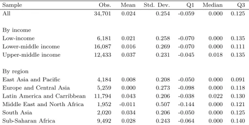
Table 2 displays (annualized) growth rate. On average, firms experience a positive
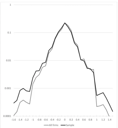
and higher in Latin American and South Asia. The distribution of growth rates typically
display heavy tails (Coad, 2009). We confirm this feature in Figure 2. We plot the
density of annual growth rates of employment for all countries (using a semi-logarithmic scale). We consider not only firms included in the analysis (black line) but also all firms available in the WBES (in grey). We confirm that the distribution of growth resembles a tent-shaped. More than 20% of firms experiences no growth and the probability mass is located around zero. Interestingly, we point out that distribution of growth for sample used in this paper is very similar to that for all firms avalaible in the WBES. This is reassuring for the representativeness of our sample.
Table 2: Descriptive statistics
Sample Obs. Mean Std. Dev. Q1 Median Q3
All 34,701 0.024 0.254 -0.059 0.000 0.125 By income Low-income 6,181 0.021 0.258 -0.070 0.000 0.135 Lower-middle income 16,087 0.016 0.269 -0.070 0.000 0.111 Upper-middle income 12,433 0.037 0.231 -0.045 0.018 0.135 By region
East Asia and Pacific 4,184 0.008 0.208 -0.050 0.000 0.091
Europe and Central Asia 5,259 0.000 0.273 -0.098 0.000 0.118
Latin America and Carribbean 11,794 0.043 0.206 -0.038 0.022 0.130 Middle East and North Africa 1,952 -0.011 0.507 -0.144 0.000 0.121
South Asia 2,020 0.034 0.206 -0.050 0.000 0.125
Sub-Saharan Africa 9,492 0.028 0.243 -0.064 0.000 0.140
Another frequent feature of firm growth distribution is the lack of persistence espe-cially for firms in the tails of the distribution, even in developing countries (Coad et al., 2018;L´eon,2020). The best performers in one period often fail to continue outperforming in the future, and inversely. We confirm this feature on an international basis by using the WBES. A simple coefficient correlation is negative (ρ = −0.10). A quantile regression confirms this finding and indicates, in line with recent papers, that persistence is lower
at the tails of the distribution (see Figure A1 in the Appendix). The lack of persistence
in growth rates raises a concern regarding the importance of (time-invariant) firm’s at-tributes in explaining growth. However, this feature does not prove that external factors matter to explain firm dynamics.
Figure 2: Distribution of firm growth (semi-logaritmic scale) 0.0001 0.001 0.01 0.1 1 -1.6 -1.4 -1.2 -1 -0.8 -0.6 -0.4 -0.2 0 0.2 0.4 0.6 0.8 1 1.2 1.4 All firms Sample
2.2.2 Determinants of firm growth: Internal vs. external factors
Our analysis seeks to distinguish between firm-level attributes and contextual variables to explain variation in growth rates across firms. To select firm-level variables we follow the previous literature on the determinants of firm growth. First we consider firm age and firm size. There is a vively debate to know if small and/or young firms experience
higher level of growth (Nichter and Goldmark, 2009;Haltiwanger et al.,2013;Aga et al.,
2015, among others). The role of foreign capital has to be taken into account as well, with foreign ownership is generally recognized as an accelerator of firm growth. Indeed,
foreign-owned firms may exhibit better growth performances due to their advantage in technology and foreign market penetration in comparison with domestic firms (Arouri et al., 2020). A burgeoining literature has pointed out the role of the characteristics of
the individual entrepreneur (Nichter and Goldmark, 2009; Woodruff, 2018) or of the
in-ternal organization of the firm (Bloom et al., 2013;McKenzie and Woodruff, 2016). Due
to the lack of relevant variables in the WBES, we consider only the experience of the manager (in the sector). These factors are, however, largely time invariant in the short-run. As a result, we include firm fixed-effects to take into account all these unobserved characteristics. We expect that these dummies will encapsulate the characteristics of the managers or owners as well as the internal organization (business practices, delegation, etc.) of the firm.
Our paper’s aim consists on analyzing whether contextual factors influence firm growth. The existing literature on the relationship between firm dynamics and their environment often specify these contextual factors (external barriers such as lack of infrastructures or corruption or external shocks such as natural disasters or conflicts). We adopt another perspective because our aim is to quantify the average weigth of these factors. In other words, we do not define specific variables but we rely on a set of dummies that take into account all unobserved factors occurring at a level of analysis.
We consider time, sector and location dummies and their interaction. Time dummies are given by the period considered for each firm. For sector, due to lack of homogeneity in data, we re-classify firms in one into 11 sectors (Wood, Garments and textiles, Chemicals products, IT, Motor vehicles, Non-metallic product, other manufacturing, trade, services, transport, and unclassified activity). For location, we extract the most precise location of firms (city or region) and create a variable reporting firm’s location inside the country. We have 363 different locations in our dataset (133 cities and 230 regions).
Based on these three sets of dummies, we create new variables accounting for differ-ent contextual factors. First, we include country-period dummies that account for all time-varying shocks occurring at the country level (such as national economic growth, institutional and political changes). Second, we consider changes at the sector-country-period level. Indeed, each sector in the same country can be affected by demand shocks
(due to a shift of demand) and/or a change in supply conditions (e.g., an increase in the price of an input, new competitors, new regulation). Finally, we include a set of dummies to take into account local changes, which can be positive (e.g., building of a new transport infrastructure, local expansion) or negative (e.g., a natural disasters). In doing so, we include (sub-national) location-period dummies.
3
Methodology
The aim of this paper is to assess the relative explanatory power of firm-level (internal) and external shocks in variability in growth. As a result, we rely on a rich literature in
management science trying to explain differences in firms’ performance (Rumelt, 1991;
Hawawini et al., 2003; Short et al., 2007; Bamiatzi et al., 2016). The basic approach
consists on exploiting an analysis of variance. The idea is to decompose total variance between explained variance by the model and the residual variance. We employ the sim-ple fixed-effects model as a model. This approach does not require to assume a specific distribution law, contrary to other variance decomposition models (such as variance
com-ponents models or mixed models).4 To get a magnitude of the ratio of explained variance
to total variance, we use the value of unajusted R2. One limitation of our approach is
the lack of rule of thumb (statistical thresholds) to indicate whether an increase in R2
is statistically significant. In addition, the order of entry of the independent variable can have a large impact on which variable explains the most variance in the dependent variable. To avoid this issue, we adopt the following approach. In a first step, we consider a simple model that includes only one constant and a variable capturing the time span
employed to compute employment growth (cf. Figure 1) as follows:
giscrt = α0+ time spant+ εiscrt (1)
4There are three different methods: fixed-effects, random-effects (also called variance components model) and mixed-effects. While the random-effects model (and the mixed-effects model) is more effi-cient, it may suffer from bias because individual unobserved heterogeneity may be correlated with the independent variables (e.g., between firm specific effect and the experience of the manager). In addition, we have to assume that random-effects follow a normal law. It should be noted that the basic decom-position of variance method have been improved in the most recent works. For instance, Short et al. (2007) employ a hierarchical linear multilevel (HLM) model because their data are nested. We cannot rely on a HLM because data are not perfectly nested in our case. Firm fixed effect is not encapsulated in country-year effect (because the latter changes over time contrary to the former).
where giscrtrefers to the growth of firm i, in sector s, in country c, in region r at the period
t; α0 is a contant and time spant is the duration considered to compute firm growth.
We consider two models allowing us to include firm-level factors. First, we then add (time varying) observable characteristics of the firm as follows:
giscrt = α0+ time spant+ ΓXit+ εiscrt (2)
where Xit refers to the time-variant characteristics of the firm: firm size (in terms of
employees) and the firm age, the manager’s experience and a dummy variable for foreign-owned firms.
We then extend Eq. 1 to consider firm time-invariant unobserved characteristics. In
doing so, we add firm fixed effects (αi) insofar as we observe a firm for at least three
periods. The estimated model becomes:
giscrt = αi+ time spant+ εiscrt (3)
The firm fixed effects allows us to control for all time-invariant firm characteristics, in-cluding firm’s internal organization but also characteristics of owners and/or managers. A major limitation of this specification is the inability to control for many time-variant unobserved characteristics (such as changes in management).
We then consider the weight of external shocks/contextual factors by adding the set of dummies presented in the previous section. We first consider a simple model adding
to Eq. 1only country-period dummies (µct) allowing us to control for factors affecting all
firms within the same country in the same period (e.g., civil conflicts, economic growth, institutional changes, etc.):
giscrt = α0+ time spant+ µct+ εiscrt (4)
We then refined Eq. 4 by considering two potential different sources of variation
within a country. On the one hand, firms operating in the same sector may be affected by a common shock which is controlled by replacing period dummies by
country-sector-period dummies (µcst) as follows:
giscrt = α0+ time spant+ µcst+ εiscrt (5)
Second, firms in the same location may be affected by a local shock that is captured by
region-period dummies (µrt):
giscrt = α0+ time spant+ µrt+ εiscrt (6)
An advantage to consider a baseline model (Eq. 1) and then include one by one
alternative independent variables is to avoid the bias induced by the order of entry that
shape value of R2. As indicated in Table 3, the comparison of R2 of different models
allows us to compute the explanatory power of different internal and external factors.
The increase of R2 from Eq. 1 to Eq. 2 gives us the variance explained by observable
firms’ characteristics and the increase of R2 from Eq. 1 to Eq. 3 by time-invariant
unobserved firms’ characteristics.
The change in R2 from Eq. 1to Eq. 4allows us to compute the role of contextual factors
at the country-period level. Eq. 5 and Eq. 6 help us to refine this analysis by focusing
on sectoral and local shocks.
Table 3: Explanatory power (R2)
From Eq. 1to Explanatory power Internal factors
→ Eq.2 Observable firm’s characteristics (age, size, sector, manager’s experience) → Eq.3 Time-invariant unobserved firm’s characteristics
External factors
→ Eq.4 Shocks common for all firms in the same country (e.g., wars, growth, institutional changes, etc.) → Eq.5 Shocks common for all firms in the same sector in the same country (e.g., regulation, etc.) → Eq.6 Shocks common for all firms in the region/city (e.g., local economic context, etc.)
For technical reasons (the large number of dummies), we rely on a linear regression
absorbing multiple levels of fixed effects (Guimaraes and Portugal,2010). This approach
does not change results regarding explanatory power. Another issue in our case is the lack of observations for sector (only one third of enterprises). As a consequence, we also
consider a restricted sample for firms with information regarding the sector.
4
Results
4.1
Baseline results
Table 4 displays baseline results based on the whole sample of firms. The first column
provides information on models (from Eq. 1 to Eq. 6 and their combinations5). The
second column gives the value of R2 (unadjusted) and the last column presents the number
of observations. Restricted refers to the sample of firms for which we have information on sector (around one third of firms only). In the rest of the table, we consider the impact of leaders and losers (see below).
Our main finding is that internal factors account for the largest share of variation in firm growth. Econometric results indicate that the combination of time-variant observable
firms’ characteristics (Eq. 2) and firm fixed effects (Eq. 3) explains more than half of
variance in employment growth. At the opposite, external factors explain less than 10% of total variance. This result is in line with the literature on the relative role of firm,
industry and country effects on performances (Hawawini et al., 2003; Short et al., 2007;
Bamiatzi et al.,2016). These papers point out the firm effect is the strongest determinants of financial performances.
Among internal factors, we also document that firm fixed effect (unobservable time-invariant characteristics) account for the largest part of explanation of total variance (around one third). This finding corroborates findings from a growing literature on firm dynamics in developing countries documenting the importance of entrepreneur
character-istics and firm internal organization (e.g., Bloom et al., 2013; McKenzie and Woodruff,
2016). In addition, as shown in Table A1 in the Appendix, we confirm results from
ex-isting papers regarding firm characteristics (Haltiwanger et al., 2013; Aga et al., 2015;
Arouri et al., 2020): small, young and foreign firms experience higher growth than their counterparts. The impact of manager experience is, however, less clear-cut.
5For instance, ”Eq2+Eq3+Eq6” refers to a model including time span
t (always included), firms’ observable characteristics from Eq. 2(Xit), firm fixed effects from Eq. 3(αi) and location-year dummies from Eq. 6(µrt). In other words, we run the following models: giscrt= αi+time spant+ΓXit+µrt+εiscrt
Table 4: Baseline results
All Excluding leaders and losers
firms Exclude both Exclude leaders Exclude losers
(1) (2) (3) (4)
R2 Obs. R2 Obs. R2 Obs. R2 Obs.
Initial value Eq1 0.002 34701 0.005 29362 0.001 30991 0.007 33072 Eq1 (restricted) 0.003 12857 0.005 10875 0.001 11445 0.007 12287 Internal factors Eq2 0.046 32308 0.035 27397 0.041 28882 0.042 30823 Eq3 0.304 33387 0.232 28323 0.269 29855 0.282 31855 Eq2+Eq3 0.555 30508 0.261 26747 0.283 28174 0.310 30044 External factors Eq4 0.054 34701 0.067 29362 0.080 30991 0.056 33072 Eq5 0.068 12857 0.086 10875 0.090 11445 0.076 12287 Eq6 0.068 34701 0.083 29362 0.095 30991 0.070 33072 Eq5+Eq6 0.097 12857 0.120 10875 0.122 11445 0.104 12287
Internal and external factors
Eq2+Eq3+Eq6 0.582 30508 0.568 25936 0.577 27292 0.587 29152
Eq2+Eq3+Eq6 (restricted) 0.650 10301 0.631 8743 0.633 9135 0.658 9909
Eq2+Eq3+Eq5+Eq6 0.658 10301 0.640 8743 0.642 9135 0.665 9909
The table displays R2of different specification. Eq1 to Eq6 refer to specification displayed in Section3and reported in Table3. Eq1 is the model with only a constant and an indicator for time span. Eq2 refers to model with observable time-variant firms’ characteristics, Eq3 to models with firm fixed effects. Eq4 to Eq6 concern external factors: Eq4 is the model with country-year dummies, Eq5 models with country-sector-year dummies and Eq6 models with region-year dummies. The combination of equation signals that we include several independent variables in the same model (e.g., Eq2+Eq3 means that we include both time-variant observable firms’ characteristics and firm fixed effects). Restricted presents model for a sample of firms for which sector variable is available.
A common feature regarding growth in that a few (high-growth) firms tend to
out-perform the rest. While many firms experience almost no growth (cf. Figure 2), a few
firms grow fast or decline sharply. The few fast-growing firms or fast-declining firms
could influence the average. To account for this issue, we follow Hawawini et al. (2003)
by excluding the top 5%-fast growing firms and the bottom 5%-fast declining firms.6
The rest of Table 4 displays results when we exclude both leaders (top 5%) and losers
(bottom 5%), and then we drop only leaders or only losers. In line with Hawawini et al.
(2003), the exclusion of leaders and losers reduces explanatory power of internal factors. This finding points out that firm effects mainly occur for top performers and bottom 6To identify these firms, we rely on annual growth for the whole period by using the number of employees in the first observation and the number of employees in the last observation divided by time-span between both observations. For instance, if we consider a firm as shown in Panel A of Figure1, we exploit information on the number of employees in 2006 and in 2012 and the period of observation is 6 years.
performers. For the sample of ”normal” firms, firms’ characteristics account for only one quarter of variance (contrary to a half when we add extreme performers). While external environment slightly increases, its explanatory power remains limited.
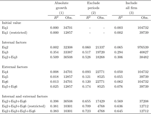
We run several robustness checks to confirm our main econometric results. First,
Erhardt(2019) shows that measurement of growth (relative vs absolute) matter to study
its dynamics. We therefore rerun models by considering absolute growth defined as the absolute difference in workers between n and t divided by the number of periods between
n and t as follows: ∆Eit = [Eit− Eit−n]/(t − n). We obtain very close results as indicated
in the first column of Table 5. Firm-level components explain one half of total variance.
However, the use of absolute growth reduces the weight of external factors to explain growth (divided by four).
Second, as indicated in the description of data and variables, we exploit three periods
of growth per firm (see Figure1). While the first and third periods cover two years, there
is a variation in the duration of the second period because the time span between two
waves differs across countries (from 3 years to 8 years as indicated in Table 1). In the
baseline analysis, we account for this issue by adding a variable (time spant). In the
second column of Table5, we keep only the first, third (and eventually the fifth) periods,
which are by definition of two years. Despite the reduction in the number of observations, we find very close results.
Third, our analysis excludes many firms for which we do not have information over different waves (because they exited before the second wave, they refused to answer
or interviewers were unable to contact them). As a result, our sample could be far
from representative of the sample of firms in developing countries. Figure 2 provides
an indirect evidence that the sample considered seems representative of all firms in the WBES in terms of employment growth. As a robustness check, we directly test whether our findings are affected by the exclusion of these non-observed firms during a second round. In doing so, we rerun the models for all firms for which we are able to compute growth rate. Our sample largely increases (from 34,701 to 104,732 observations). Our
findings, displayed in the third column of Table 5, are largely unchanged for the impact
(certainly because we cannot employ firm fixed effects for the majority of firms).
Table 5: Robustness checks
Absolute Exclude Include
growth periods all firm
(1) (2) (3)
R2 Obs. R2 Obs. R2 Obs.
Initial value Eq1 0.000 34701 - - 0.003 104732 Eq1 (restricted) 0.000 12857 - - 0.002 39739 Internal factors Eq2 0.002 32308 0.060 21337 0.065 976539 Eq3 0.354 33387 0.517 19720 0.294 40827 Eq2+Eq3 0.509 30508 0.528 18268 0.306 38482 External factors Eq4 0.008 34701 0.093 22771 0.050 104732 Eq5 0.018 12857 0.121 8525 0.055 39739 Eq6 0.013 34701 0.120 22771 0.062 104732 Eq5+Eq6 0.025 12857 0.174 8525 0.076 39739
Internal and external factors
Eq2+Eq3+Eq6 0.398 30508 0.655 17429 0.569 37208
Eq2+Eq3+Eq6 (restricted) 0.381 10301 0.709 4768 0.636 12712
Eq2+Eq3+Eq5+Eq6 0.383 10301 0.723 4768 0.645 12712
The table displays R2 of different specification. Eq1 to Eq6 refer to specification displayed in Section3and reported in Table3. Eq1 is the model with only a constant and an indicator for time span. Eq2 refers to model with observable time-variant firms’ characteristics, Eq3 to models with firm fixed effects. Eq4 to Eq6 concern external factors: Eq4 is the model with country-year dummies, Eq5 models with country-sector-year dummies and Eq6 models with region-year dummies. The combination of equation signals that we include several independent variables in the same model (e.g., Eq2+Eq3 means that we include both time-variant observable firms’ characteristics and firm fixed effects). Restricted presents model for a sample of firms for which sector variable is available.
4.2
Extensions
4.2.1 Heterogeneity
We extend our analysis by examining how firm structural characteristics and country attributes influence the relative weight of internal and external factors in explaining vari-ance of firm growth. We first consider the importvari-ance of firm attributes, especially their
size, age and industry.7 For size, we consider classification given by the WBES: Small
firms (less than 20 employees), Medium firms (between 20 and 99 employees) and Large 7In an unreported analysis, we also distinguish foreign firms and domestic firms. However, the differ-ence in sample is too large to be able to compare R2.
firms (more than 100 employees). For age, we consider age at the beginning of the period and classify firms into four groups: New firms (less than 5 year-old), Young (between 5 and 9 year-old), Medium (between 10 and 19 year-old) and Old (more than 20-year old). Finally, for industry we consider manufacturing and services. We cannot compare results with the global sample but rather between sub-sample.
Figure 3: Sensitivity to firm characteristics
0 0.05 0.1 0.15 0.2 0.25 0.3 0.35 0.4 0.45 0.5
Small Medium Large Manufacturing Services New Young Medium Old
Internal External
According to findings displayed in Figure 3(see Table A2for details), we find no real
difference between firms according to their size or sector. The analysis by age is, however, interesting. While internal factors explain more or less the same share of total variance for different groups (dark bars), young firms are more sensitive to external factors (light bars). External factors explain one quarter of variation for new firms (below 5-year old) but less than 15% for old firms (more than 20-year old). In other words, while external context does not matter a lot to explain differences in growth, it seems more crucial for
new and young firms. This result is in line with Coad et al. (2018) indicating that old firms are more able to sustain their previous growth than new firms.
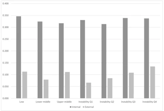
We then consider the role of country-level attributes. We first take into account the income-level, which is a proxy for many unobserved differences across countries (institu-tions, infrastructure, financial development, etc.). We may expect that firms in richer countries benefit from better business conditions than those operating in low-income countries. We also consider the degree of instability in the country. We expect that countries impacted by external (positive or negative) shocks, irrespective of their nature, will present higher level of output instability. To compute output instability (at a macro-level), we rely on a very simple proxy: the standard deviation of growth from 1995 to
2018.8
Results, presented in Figure4, do not signal strong differences according to the level of
income. Internal factors seem to be more important in poor economies but this finding is
not robust (see TableA3in the Appendix). The relative importance of external factors is
more or less similar for firms in different income-level categories (their impact is reduced for middle category).
Findings from classification of countries according to their level of output instability is much interesting. The first quartile groups together countries with a lower variability in output, and fourth quartile is made up of the most unstable countries. First, while we may expect that unobserved individual characteristics matter a lot to operate in unstable market, we fail to find a clear difference in the explanatory power of internal factors. As expected, external factors are more important in chaotic environment. The contribution of external factors in explaining variance doubles between firms operating in the most stable countries to those in the most unstable economies.
To sum up, our findings indicate that young firms and those operating in unstable countries are more sensitive to external shocks. However, the role played by individual 8We also consider more refined indicator of output volatility by using the sum of squared residual of regressions of growth to past growth and a trend for each country (see Cariolle and Goujon, 2015, for a discussion on the best way to measure instability). This measure is highly correlated with simple standard deviation (ρ = 0.91) and, consequently, results (available upon request) are very similar when we consider this alternative measure of output instability.
Figure 4: Sensitivity to country characteristics 0.000 0.050 0.100 0.150 0.200 0.250 0.300 0.350 0.400
Low Lower middle Upper middle Instability Q1 Instability Q2 Instability Q3 Instability Q4 Internal External
factors is weakly shaped when we consider different sub-samples.
4.2.2 Firm exit
Finally, we scrutinize how internal and external factors influence firm exit. One might argue that the primary aim of small firm’s managers is to maintain their business alive without seeking to grow. As a result, observing that many firms do not grow is rather normal. Firm performance could be weakly correlated to (local and sectoral) shocks because managers do not exploit positive shocks or because managers have developed strategies to cope with negative events. However, one might expect that firm survival is
sensitive to economic environment (Aga and Francis, 2017). In period of booms, more
firms may be able to stay in the market. At the opposite, during crises, many enterprises leave the floor. In the following, we study whether external factors matter more for firm survival than for firm growth. While we are also interested by the role of firm internal factors in explaining exit, we are limited by our dataset. By construction, we have only
one observation per firm and therefore cannot include firm level control variables.
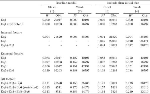
The WBESs are not dedicated to study exit. We follow the methodology developed
by Aga and Francis (2017) to define exit. The method uses the reason reported by the
interviewer when she was unable to recontact a firm. Firms are classifed into three groups. The first group includes firms which continue to operate. The second group is made up of firms that are known to have exited the market (closed or bankrupt). The third group consists of firms for which operating status is uncertain (refuse a follow-up interview or
are unavailable). Based on these categories,Aga and Francis (2017) create two variables
of exit. The first variable is a strict exit that consider only the sample of firms for which status is clear-cut (exited or continuing firms). The second exit dummy (weak) adds as exiters firms with an uncertain status.
Table 6: Determinants of firm exit
Baseline model Include firm initial size
Strict Weak Strict Weak
(1) (2) (3) (4)
R2 Obs. R2 Obs. R2 Obs. R2 Obs.
Eq1 0.000 26047 0.000 42191 0.000 26047 0.000 42191 Eq1 (restricted) 0.000 10263 0.000 16797 0.000 10263 0.000 16797 Internal factors Eq2 0.004 21820 0.004 35403 0.004 21820 0.004 35403 Eq3 - - - - 0.015 22056 0.010 35171 Eq2+Eq3 - - - - 0.024 19021 0.017 30176 External factors Eq4 0.083 26047 0.122 42191 0.083 26047 0.122 42191 Eq5 0.097 10263 0.152 16797 0.097 10263 0.152 16797 Eq6 0.106 26047 0.151 42191 0.106 26047 0.151 42191 Eq5+Eq6 0.139 10263 0.188 16797 0.139 10263 0.188 16797 All factors Eq2+Eq3+Eq6 0.111 21820 0.150 35403 0.121 19021 0.173 30176 Eq2+Eq3+Eq6 (restricted) 0.135 8511 0.176 14079 0.157 7429 0.204 12010 Eq2+Eq3+Eq5+Eq6 0.143 8511 0.183 14079 0.164 7429 0.210 12010
The table displays R2of different specification. The dependent variable is a dummy for exit, according to two definitions (see Section 4.3.2). Eq1 to Eq6 refer to specification displayed in Section3and reported in Table3. Eq1 is the model with only a constant and an indicator for time span. Eq2 refers to model with observable time-variant firms’ characteristics, Eq3 to models with firm initial size. Eq4 to Eq6 concern external factors: Eq4 is the model with country-year dummies, Eq5 models with country-sector-year dummies and Eq6 models with region-year dummies. The combination of equation signals that we include several independent variables in the same model (e.g., Eq2+Eq3 means that we include both time-variant observable firms’ characteristics and firm fixed effects). Restricted presents model for a sample of firms for which sector variable is available.
weak). Despite the binary structure of dependent variables, we employ a probability linear model allowing us to compute the share of total variance explained by the model. Unfortunately, we cannot include firm fixed effects because we have one observation per firm. To overcome this issue, we include firm initial size (a set of dummies for each size) in columns (3) and (4). We might expect that initial size captures many unobserved
firm’s time-invariant characteristics (Ayyagari et al., 2017, 2020). In addition, there is
large literature indicating that initial conditions shape the likelihood to survive (Geroski et al., 2010).
Results, displayed in the last two columns of Table5, are instructive. We cannot
dire-cly compare the importance of internal factors due to the omission of firm-level dummies. Even with the inclusion of firm initial size in the last two columns, firm-level
character-istics do not seem to matter (R2 < 0.025). Results, displayed in Appendix (Table A4),
largely confirm those reported byAga and Francis(2017). Large and old firms as well as
those lead by experienced managers are more likely to survive. We also fail to detect a difference between foreign-owned and domestic-owned firms.
Interestingly, the impact of external factors seems stronger for exit than for growth. This finding is just suggestive due to differences in models. In addition, the explanatory power of external factors remains rather limited because it explains less than 20% of total variance. In other words, our econometric results suggest that external shocks are more stronger to explain variance in firm exit than variance in firm growth. However, these findings should be treated with caution because models are not directly comparable.
5
Conclusion
The Covid crisis has highlighted the importance of external shocks on firm dynamics worldwide. Developing countries are often hurt by major external shocks that may impede the development of a sound private sector. Our paper examines the relative weight of internal firm characteristics and external shocks to explain variation of firm growth. In doing so, we exploit a rich firm-level panel database from the World Bank Enterprise Surveys combining information on employment growth of 12,562 firms operating in 72 low and middle-income countries. Our approach is data-driven insofar as we do not
explicit internal and external factors but rather assess their explanatory power by block. Our main findings can be summarized as follows. We show that internal factors, es-pecially time-invariant firm characteristics, explain a half of differences in firm growth. However, the role of internal factors is predominant for leaders (best performers in the long-run) and losers (worst performers). When we exclude leaders and losers the con-tribution of internal factors is halved. The external shocks at the sector or local level account for less than 10% of differences in variation on average. Third, the impact of in-ternal factors is weakly shaped by firm-level and country-level characteristics, contrary to the role played by external factors. In particular, external factors are more important for new and young firms and for firms operating in unstable environments. Finally, primary econometric results suggest that external shocks are more important to explain exit than growth.
Our statistical analysis provides interesting results regarding the relative weight of internal firm characteristics versus external shocks to explain firm dynamics. However, one might keep in mind that findings are only an average effect. In other words, some shocks can have a profound impact for firms. In addtiion, we do not consider the inter-action between internal factors and exogenous events. Recent evidence points out that specific ex-ante firm-level attributes are particularly important to favor firm recovery
af-ter a shock (e.g., Bowles et al., 2016; Dosso and L´eon, 2020). Future works should go
forward to by investigating firm’s reaction to a specific event. In particular, we should focus on how firms in developing countries cope with shocks before a shock by adoption risk mitigation strategies or after the occurrence of a shock through coping actions.
References
Aga, G. and Francis, D. (2017). As the market churns: estimates of firm exit and job loss using the world bank’s enterprise surveys. Small Business Economics, 49:379–403. Aga, G., Francis, D. C., and Meza, J. R. (2015). Smes, age, and jobs: A review of the
Arouri, H., Youssef, A. B., Quatraro, F., and Vivarelli, M. (2020). Drivers of growth in tunisia: Young firms vs incumbents. Small Business Economics, 54:323–340.
Ayyagari, M., Demirguc-Kunt, A., and Maksimovic, V. (2017). What determines en-trepreneurial outcomes in emerging markets? the role of initial conditions. The Review of Financial Studies, 30(7):2478–2522.
Ayyagari, M., Demirguc-Kunt, A., and Maksimovic, V. (2020). Are large firms born or made? evidence from developing countries. Small Business Economics, forthcoming. Bamiatzi, V., Bozos, K., Cavusgil, S. T., and Hult, G. T. M. (2016). Revisiting the firm,
industry, and country effects on profitability under recessionary and expansion periods: A multilevel analysis. Strategic Management Journal, 37(7):1448–1471.
Beck, T. and Demirguc-Kunt, A. (2006). Small and medium-size enterprises: Access to finance as a growth constraint. Journal of Banking & finance, 30(11):2931–2943. Bloom, N., Eifert, B., Mahajan, A., McKenzie, D., and Roberts, J. (2013). Does
manage-ment matter? evidence from india. The Quarterly Journal of Economics, 128(1):1–51. Bloom, N. and Van Reenen, J. (2007). Measuring and explaining management practices
across firms and countries. The Quarterly Journal of Economics, 122(4):1351–1408. Bowles, J., Hjort, J., Melvin, T., and Werker, E. (2016). Ebola, jobs and economic
activity in liberia. Journal of Epidemiology & Community Health, 70(3):271–277. Cariolle, J. and Goujon, M. (2015). Measuring macroeconomic instability: A critical
survey illustrated with exports series. Journal of Economic Surveys, 29(1):1–26. Coad, A. (2009). The growth of firms: A survey of theories and empirical evidence.
Edward Elgar Publishing.
Coad, A., Daunfeldt, S.-O., and Halvarsson, D. (2018). Bursting into life: firm growth and growth persistence by age. Small Business Economics, 50(1):55–75.
Cole, M. A., Elliott, R. J., Occhiali, G., and Strobl, E. (2018). Power outages and firm performance in sub-saharan africa. Journal of Development Economics, 134:150–159.
Dosso, I. and L´eon, F. (2020). Civil conflict and firm recovery: Evidence from
post-electoral crisis in Cˆote d’Ivoire. FERDI Working Paper, 266:1–46.
Easterly, W., Kremer, M., Pritchett, L., and Summers, L. H. (1993). Good policy or good luck? country growth performance and temporary shocks. Journal of Monetary Economics, 32(3):459–483.
Elliott, R. J., Liu, Y., Strobl, E., and Tong, M. (2019). Estimating the direct and indi-rect impact of typhoons on plant performance: Evidence from chinese manufacturers. Journal of Environmental Economics and Management, 98:102252.
Erhardt, E. C. (2019). Measuring the persistence of high firm growth: choices and
consequences. Small Business Economics, forthcoming:1–28.
Eslava, M., Haltiwanger, J. C., and Pinz´on, A. (2019). Job creation in Colombia vs the
US:“up or out dynamics” meets “the life cycle of plants”. NBER Working Paper, 25550. Fisman, R. and Svensson, J. (2007). Are corruption and taxation really harmful to
growth? firm level evidence. Journal of Development Economics, 83(1):63–75.
Geroski, P. A., Mata, J., and Portugal, P. (2010). Founding conditions and the survival of new firms. Strategic Management Journal, 31(5):510–529.
Guimaraes, P. and Portugal, P. (2010). A simple feasible procedure to fit models with high-dimensional fixed effects. Stata Journal, 10(4):628–649.
Haltiwanger, J., Jarmin, R. S., and Miranda, J. (2013). Who creates jobs? small versus large versus young. Review of Economics and Statistics, 95(2):347–361.
Hausmann, R., Pritchett, L., and Rodrik, D. (2005). Growth accelerations. Journal of Economic Growth, 10(4):303–329.
Hawawini, G., Subramanian, V., and Verdin, P. (2003). Is performance driven by
industry-or firm-specific factors? a new look at the evidence. Strategic Management Journal, 24(1):1–16.
Hsieh, C.-T. and Klenow, P. J. (2014). The life cycle of plants in india and mexico. The Quarterly Journal of Economics, 129(3):1035–1084.
Hsieh, C.-T. and Olken, B. A. (2014). The missing ”missing middle”. Journal of Economic Perspectives, 28(3):89–108.
Klapper, L., Laeven, L., and Rajan, R. (2006). Entry regulation as a barrier to en-trepreneurship. Journal of Financial Economics, 82(3):591–629.
L´eon, F. (2020). The elusive quest for high-growth firms in Africa: When other metrics
of performance say nothing. Small Business Economics, forthcoming:1–32.
McKenzie, D. and Woodruff, C. (2016). Business practices in small firms in developing countries. Management Science, 63(9):2773–3145.
Nichter, S. and Goldmark, L. (2009). Small firm growth in developing countries. World Development, 37(9):1453–1464.
Pritchett, L. (2000). Understanding patterns of economic growth: searching for hills among plateaus, mountains, and plains. World Bank Economic Review, 14(2):221–250. Rodrik, D. (1999). Where did all the growth go? external shocks, social conflict, and
growth collapses. Journal of Economic Growth, 4(4):385–412.
Rumelt, R. P. (1991). How much does industry matter? Strategic Management Journal, 12(3):167–185.
Short, J. C., Ketchen Jr, D. J., Palmer, T. B., and Hult, G. T. M. (2007). Firm, strate-gic group, and industry influences on performance. Stratestrate-gic Management Journal, 28(2):147–167.
Woodruff, C. (2018). Addressing obstacles to small and growing businesses. IGC Working paper, pages 1–35.
Online Appendix
Firm growth in developing countries: Driven by external shock of
internal characteristics?
Figure A1: Firm growth persistence, quantile regression
The figure plots the coefficient associated with lagged growth (in red) and confidence intervals (in grey) using quantile regression where the dependant variable is current growth.
T a b le A1 : Ba sel in e res u lts , com p le te ta b le Base line In ternal fa ctors E xt erna l A ll E q1 E q1 (rest ) Eq 2 Eq 3 E q2 +3 E q 4 E q 5 Eq 6 Eq 5 +6 E q2 +3+ 6 Eq 2+ 3+6 (rest ) E q 2+3 +5+ 6 Ti me sp an -0.0 13* ** -0.0 15** * -0.0 11* ** -0.0 20* ** -0.0 08** * -0.0 12* ** -0.0 16* ** -0.0 12** * -0.01 6** * -0.0 01 -0.0 08* ** -0.0 08** * (0. 001 ) (0 .003 ) (0.0 01) (0. 002) (0 .001 ) (0.0 02) (0.0 03) (0 .002 ) (0 .003 ) (0.0 02) (0. 003) (0 .003 ) Siz e -0.0 39* ** -0 .267 *** -0.2 69* ** -0.30 5** * -0.30 8** * (0 .001 ) (0.0 03) (0.00 3) (0.0 05) (0. 005) A ge -0 .00 3 -0.0 29* ** -0 .040 *** -0 .029 *** -0 .032 *** (0 .002 ) (0.0 03) (0.00 3) (0.0 07) (0. 007) F or eign 0 .051 *** 0.04 9*** 0.0 40* ** 0.09 0** * 0 .087 *** (0 .005 ) (0.0 09) (0.00 9) (0.0 20) (0. 020) M an ag. E x p. 0.0 03 0 .003 0.01 0** * 0 .011 0. 013 * (0 .002 ) (0.0 04) (0.00 4) (0.0 07) (0. 007) Firm FE Y es Y es Y es Y es Y es Co un try-Y e ar FE Y es Co un try-Sect or-Y ea r FE Y es Y es Y es L o cat ion-Y e ar FE Y es Y e s Y e s Y es Y es Ob s. 3470 1 1285 7 323 08 333 87 305 08 3 4701 12 857 34 701 12 857 3 050 8 1 030 1 1 030 1 R 2 0.0 03 0.0 03 0.0 46 0.30 3 0.55 5 0.05 4 0 .06 8 0 .068 0.0 97 0 .582 0.6 50 0.6 58 F-t est 85.8 *** 38 .8** * 311 .0** * 1 49.5 *** 21 70.6 *** 1 2.4 *** 3.3 *** 4.0 *** 1.8 *** 3 0.4* ** 15. 1** * 1 2.7* ** Th e table rep orts co e fficie n ts asso ciate d w ith tim e sp an and fi rm-le v e l v ari ables . Th e lab el ref ers to tho se rep o rted in T ab le 4 . A ll fix ed -eff ects are in clud ed when in dica ted but un rep o rted. *, ** , *** ref er to signifi can ce at the 1 0%, 5 % an d 1% lev el, re sp ec tiv ely
Table A2: Contribution of internal and external factors, by group of firms
Size Industry
Small Medium Large Manufact. Services
R2 Obs. R2 Obs. R2 Obs. R2 Obs. R2 Obs.
Initial value Eq1 0.002 15101 0.003 12022 0.003 7578 0.003 8347 0.004 4130 Eq1 (restricted) 0.001 4806 0.005 4649 0.003 3402 - - - -Internal factors Eq2 0.347 13934 0.414 11286 0.231 7088 0.054 7707 0.044 3892 Eq3 0.334 13713 0.368 10397 0.376 6836 0.363 7066 0.349 3424 Eq2+Eq3 0.374 12703 0.454 9938 0.396 6550 0.373 6628 0.376 3274 External factors Eq4 0.107 15101 0.057 12022 0.059 7578 0.061 8347 0.049 4130 Eq5 0.134 4806 0.104 4649 0.114 3402 0.068 8347 0.060 4130 Eq6 0.129 15101 0.091 12022 0.104 7578 0.103 8347 0.079 4130 Eq5+Eq6 0.189 4806 0.171 4649 0.183 3402 0.108 8347 0.089 4130
Internal and external factors
Eq2+Eq3+Eq6 0.708 12374 0.772 9636 0.719 6300 0.699 6453 0.625 3167
Eq2+Eq3+Eq6 (restricted) 0.735 3557 0.787 3507 0.741 2675 - - -
-Eq2+Eq3+Eq5+Eq6 0.740 3557 0.790 3507 0.751 2675 0.700 6453 0.631 3167
Age
New Young Medium Old
R2 Obs. R2 Obs. R2 Obs. R2 Obs.
Initial value Eq1 0.007 7314 0.005 7225 0.001 9734 0.001 9772 Eq1 (restricted) 0.008 2617 0.004 2453 0.002 8611 0.001 8928 Internal factors Eq2 0.062 6755 0.045 6783 0.039 9214 0.043 9056 Eq3 0.314 7048 0.274 6913 0.292 9366 0.308 9433 Eq2+Eq3 0.348 6512 0.315 6547 0.302 8954 0.343 8979 External factors Eq4 0.088 7314 0.077 7225 0.056 9734 0.062 9772 Eq5 0.157 2617 0.146 2453 0.097 3611 0.089 3928 Eq6 0.135 7314 0.128 7225 0.094 9734 0.092 9772 Eq5+Eq6 0.245 2617 0.240 2453 0.179 3611 0.146 3928
Internal and external factors
Eq2+Eq3+Eq6 0.645 6361 0.593 6383 0.586 8734 0.589 8557
Eq2+Eq3+Eq6 (restricted) 0.711 2100 0.682 1913 0.684 2953 0.664 3155
Eq2+Eq3+Eq5+Eq6 0.725 2100 0.699 1913 0.701 2953 0.684 3155
The dependent variable is the absolute growth in column (1), the relative growth in column (2) and two exit dummies in the remaining columns. The table displays R2 of different specification. Eq1 to Eq6 refer to specification displayed in Section3and reported in Table3. Eq1 is the model with only a constant and an indicator for time span. Eq2 refers to model with observable time-variant firms’ characteristics, Eq3 to models with firm fixed effects. Eq4 to Eq6 concern external factors: Eq4 is the model with country-year dummies, Eq5 models with country-sector-country-year dummies and Eq6 models with region-country-year dummies. The combination of equation signals that we include several independent variables in the same model (e.g., Eq2+Eq3 means that we include both time-variant observable firms’ characteristics and firm fixed effects). Restricted presents model for a sample of firms for which sector variable is available.
T a b le A3 : Con tr ib u ti on o f in ter n a l an d ext er n a l fa ct or s, b y co u n try ch ar a ct er ist ics Incom e lev el De gree of insta bilit y L o w L o w e r midd le U pp er midd le 1s t q uarti le 2nd q u artile 3rd qu artile 4t h q uart ile R 2 O bs. R 2 O bs. R 2 O bs. R 2 Obs. R 2 Obs. R 2 Obs. R 2 Ob s. E q1 0 .001 61 81 0. 003 160 87 0. 002 12 433 0 .002 11 347 0 .002 83 07 0.0 04 722 1 0.00 2 782 6 E q1 (rest ricte d) 0 .00 0 21 42 0 .005 58 28 0.0 02 488 7 0.00 3 4 313 0 .00 1 28 47 0 .003 26 87 0.0 03 30 10 In ter nal fact ors E q2 0 .072 56 50 0. 042 148 88 0. 045 11 770 0 .033 10 694 0 .041 78 66 0.0 53 658 6 0.07 5 716 2 E q3 0 .305 59 07 0. 313 154 16 0. 286 12 007 0 .322 10 961 0 .280 79 82 0.3 00 690 4 0.30 0 754 0 E q2 +E q 3 0 .34 6 53 37 0 .324 14 504 0 .317 11 573 0 .330 10 483 0 .314 77 46 0. 339 628 7 0.3 37 69 55 E xt erna l fa ctor s E q4 0 .083 61 81 0. 036 160 87 0. 064 12 433 0 .023 11 347 0 .005 83 07 0.0 71 722 1 0.08 5 782 6 E q5 0 .081 21 42 0. 052 582 8 0.0 83 488 7 0.43 4 4 313 0 .063 28 47 0. 069 268 7 0.1 03 30 10 E q6 0 .097 61 81 0. 047 160 87 0. 083 12 433 0 .031 11 347 0 .064 83 07 0.0 89 722 1 0.10 5 782 6 E q5 +E q 6 0 .11 3 21 42 0 .079 58 28 0.1 11 488 7 0.06 6 4 313 0 .08 5 28 47 0 .108 26 87 0.1 35 30 10 A ll fact ors E q2 +E q 3+E q 6 0.57 7 5 240 0 .572 13 962 0 .605 11 249 0 .548 10 128 0 .575 74 76 0. 616 61 37 0.6 21 67 67 E q2 +E q 3+E q 6 (re strict ed) 0.61 7 1 616 0 .624 47 48 0. 694 39 24 0.6 09 365 7 0.67 6 2 120 0 .680 20 93 0. 679 2 431 E q2 +E q 3+E q 5+E q 6 0.62 2 1 616 0 .646 47 48 0. 698 39 24 0.6 22 365 7 0.68 0 2 120 0 .683 20 93 0. 687 2 431 Th e d ep en den t v aria ble is th e re lativ e gro w th. T he tabl e di spla y s R 2 of d iff eren t sp e cifica tion . Eq 1 to Eq 6 ref er to sp ecifi catio n d ispla y e d in Se ction 3 and rep orted in T a ble 3 . E q1 is the m o del w ith o nly a con stan t a nd an indic ator for time sp an. Eq 2 re fer s to mo del wi th obs erv able time-v a rian t firms ’ chara cteri stics, Eq 3 to mo d els wi th fir m fix ed eff ect s. E q 4 to Eq 6 c onc ern ex te rnal fa ctor s: E q 4 is the m o de l wit h cou n try -y ea r du mmie s, E q 5 mo dels with cou n try -se ctor-y e ar du mm ies an d E q 6 mo dels wi th reg ion-y e ar dum mie s. T he co m bi nati on of eq ua tion si gna ls that w e inc lude sev eral in dep e nden t v aria bles in the sam e mo del (e .g., Eq 2 +E q3 mea ns tha t w e in clud e b o th ti me-v ar ian t o bser v a ble fi rms’ chara cteris tics an d fir m fix ed eff ects) . Res tricte d pre sen ts mo d el for a sa mp le of firm s for wh ic h se ctor v a riabl e is a v ail able .
Table A4: Determinants of firm survival
Exit strict Exit weak
Eq2+Eq3 Eq2+Eq3 Eq2+Eq3 Eq2+Eq3 Eq2+Eq3 Eq2+Eq3
+Eq6 +Eq5+Eq6 +Eq6 +Eq5+Eq6
(1) (2) (3) (4) (5) (6) Time span -0.018* -0.008 0.004 -0.004 0.004 0.001 (0.010) (0.011) (0.019) (0.013) (0.015) (0.027) Size (log) 0.015*** 0.016*** 0.015*** 0.017*** 0.021*** 0.020*** (0.002) (0.002) (0.004) (0.003) (0.003) (0.005) Age (log) 0.007*** 0.010*** 0.009** 0.025*** 0.026*** 0.018*** (0.003) (0.003) (0.004) (0.004) (0.004) (0.006) Foreign 0.003 0.002 -0.00 0.019* 0.004 -0.020 (0.008) (0.008) (0.012) (0.010) (0.010) (0.016)
Manag. Exp. (log) 0.013*** 0.014*** 0.013** 0.016*** 0.023*** 0.021***
(0.004) (0.004) (0.006) (0.005) (0.005) (0.007)
Birth size Yes Yes Yes Yes Yes Yes
Location-Year FE No Yes Yes No Yes Yes
Country-Sector-Year FE No No Yes No No Yes
Obs. 19021 19021 7429 30176 30176 12010
R2 0.024 0.121 0.164 0.017 0.173 0.210
The dependent variable is a dummy equals to 1 if a firm survive and 0 if a firm exit. Eq2 refers to model with observable time-variant firms’ characteristics, Eq3 to models with firm fixed effects. Eq5 models with country-sector-year dummies and Eq6 models with region-year dummies. The combination of equation signals that we include several independent variables in the same model (e.g., Eq2+Eq3 means that we include both time-variant observable firms’ characteristics and firm fixed effects). *, **, *** refer to significance at the 10%, 5% and 1% level, respectively