Publisher’s version / Version de l'éditeur:
Vous avez des questions? Nous pouvons vous aider. Pour communiquer directement avec un auteur, consultez la
première page de la revue dans laquelle son article a été publié afin de trouver ses coordonnées. Si vous n’arrivez
Questions? Contact the NRC Publications Archive team at
PublicationsArchive-ArchivesPublications@nrc-cnrc.gc.ca. If you wish to email the authors directly, please see the first page of the publication for their contact information.
https://publications-cnrc.canada.ca/fra/droits
L’accès à ce site Web et l’utilisation de son contenu sont assujettis aux conditions présentées dans le site LISEZ CES CONDITIONS ATTENTIVEMENT AVANT D’UTILISER CE SITE WEB.
Laboratory Memorandum; no. LM-2004-02, 2004
READ THESE TERMS AND CONDITIONS CAREFULLY BEFORE USING THIS WEBSITE. https://nrc-publications.canada.ca/eng/copyright
NRC Publications Archive Record / Notice des Archives des publications du CNRC :
https://nrc-publications.canada.ca/eng/view/object/?id=5ba44a3a-57d2-4e7a-a482-48fc4129571b https://publications-cnrc.canada.ca/fra/voir/objet/?id=5ba44a3a-57d2-4e7a-a482-48fc4129571b
Archives des publications du CNRC
For the publisher’s version, please access the DOI link below./ Pour consulter la version de l’éditeur, utilisez le lien DOI ci-dessous.
https://doi.org/10.4224/8895502
Access and use of this website and the material on it are subject to the Terms and Conditions set forth at
Standard Monohull Resistance Experiments: Investigation of Issues Related to the Derivation of the Prohaska Form Factor
Ocean Technology technologies oc ´eaniques
Laboratory Memorandum
LM-2004-02
Standard Monohull Resistance Experiments: Investigation
of Issues Related to the Derivation of the Prohaska Form
Factor
Cumming, D., Pallard, R. and Molyneux, W. D.
March 2004
REPORT NUMBER
LM-2004-02
NRC REPORT NUMBER DATE
March 2004
REPORT SECURITY CLASSIFICATION
Unclassified
DISTRIBUTION
Unlimited
TITLE
STANDARD MONOHULL RESISTANCE EXPERIMENTS: INVESTIGATION OF ISSUES RELATED TO THE DERIVATION OF THE PROHASKA FORM FACTOR
AUTHOR(S)
D. Cumming, R. Pallard, D. Molyneux
CORPORATE AUTHOR(S)/PERFORMING AGENCY(S)
Institute for Ocean Technology, National Research Council, St. John’s, NL
PUBLICATION
N/A
SPONSORING AGENCY(S)
Institute for Ocean Technology, National Research Council, St. John’s, NL
IMD PROJECT NUMBER
42_960_26
NRC FILE NUMBER
KEY WORDS
Prohaska, Form Factor, Resistance
PAGES iv, 9 FIGS. 14 TABLES 1 SUMMARY
This report describes an investigation into the procedure IOT currently uses to evaluate Prohaska’s form factor during a standard open water resistance test analysis. Three issues were investigated:
1) Adopting Chauvenet’s Criterion for evaluating data outliers during the Prohaska form factor determination.
2) The influence of immersed transom on form factor. 3) The influence of adding appendages on form factor.
4) Using a higher order power on Fr in the Prohaska form factor plot.
Data from a number of resistance experiments will be used to investigate each issue and recommendations will be made to improve the existing resistance analysis software.
ADDRESS National Research Council
Institute for Ocean Technology Arctic Avenue, P. O. Box 12093 St. John's, NL A1B 3T5
Institute for Ocean Institut des technologies Technology océaniques
STANDARD MONOHULL RESISTANCE EXPERIMENTS:
INVESTIGATION OF ISSUES RELATED TO THE DERIVATION OF THE
PROHASKA FORM FACTOR
LM-2004-02
D. Cumming, R. Pallard, D. Molyneux
TABLE OF CONTENTS
List of Tables... ii
List of Figures ... ii
List of Abbreviations/Symbols... iii
1.0 INTRODUCTION ... 1
2.0 BACKGROUND ... 1
3.0 DETERMINATION OF THE PROHASKA FORM FACTOR... 2
4.0 DESCRIPTION OF EXISTING IOT BARE HULL FORM FACTOR ANALYSIS SOFTWARE ... 3
5.0 APPLYING CHAUVENET’S CRITERION ... 3
6.0 DISCUSSION ... 4
6.1 Chauvenet’ Criterion... 4
6.2 Transom Stern Issues ... 5
6.3 Influence of Appendages on Prohaska Form Factor... 5
6.4 Deriving the Prohaska Form Factor on Full Hull Forms ... 6
7.0 RECOMMENDATIONS... 6
7.1 Chauvenet’ Criterion... 6
7.2 Transom Sterns ... 7
7.3 Appended Models ... 7
7.4 Full Hull Forms... 7
8.0 ACKNOWLEDGEMENTS... 8
LIST OF TABLES
Table
Chauvenet’s Criterion for Rejecting a Data Point……….………….1
LIST OF FIGURES Figure Typical Prohaska Form Factor Plot Output by IOT Standard Analysis Software………....….1
IOT Standard Resistance Analysis Software: Prohaska Form Factor………….…..…2
IOT Standard Resistance Analysis Software: Selection of Froude Number Range and Fr Power………..….…3
Chauvenet’s Criterion: Relationship Between Number of Points N and Maximum Acceptable Criterion……….…...…..4
Prohaska Plot with Identified Outlier………...…...…..5
Prohaska Plot (Figure 5) with Outlier Removed……….…..6
Prohaska Data With/Without Transom Stern Immersed……….……..7
Photograph of Laker With Dummy Z-Drives Fitted……….8
Prohaska Form Factor Plot – Bulk Carrier With/Without Z-drives………..9 Prohaska Plots for Full Form Vessel – Frn where n = 4,5,6,8, and 10………….10 - 14
LIST OF ABBREVIATIONS/SYMBOLS
ABS absolute value
CB block coefficient
CFM frictional resistance coefficient for the model
CTM total resistance coefficient for the model
CR residuary resistance coefficient
Fr Froude Number
g gravitational acceleration (standard IOT value 9.808 m/s2)
IOT Institute for Ocean Technology
ITTC International Towing Tank Conference
1 + k form factor
kW kiloWatt(s)
LM model length on the water line (m)
m metre(s)
N number of samples, Newton(s)
PE effective power (kW)
ReM Reynold’s Number for the model
RTM total resistance for the model (N)
s second(s)
SNAME Society of Naval Architects and Marine Engineers SM wetted surface area of the model (m2)
LIST OF ABBREVIATIONS/SYMBOLS (cont’d)
VM model speed (m/s)
ρM water density for the model test facility (kg/m3)
τ nondimensional deviation (Chauvenet’s Criterion)
STANDARD MONOHULL RESISTANCE EXPERIMENTS: INVESTIGATION OF ISSUES RELATED TO THE DERIVATION OF THE PROHASKA FORM
FACTOR 1.0 INTRODUCTION
This report describes an investigation into the procedure IOT uses to evaluate Prohaska’s form factor during a standard open water resistance test analysis. Four issues were investigated:
1) Adopting Chauvenet’s Criterion described in Reference 1 for evaluating data outliers during the Prohaska form factor determination.
2) The influence of immersed transom on form factor. 3) The influence of adding appendages on form factor.
4) Using a higher order power ‘n’ on Frn in the Prohaska form factor plot.
Data from a number of resistance experiments were used to investigate these issues and recommendations are made to amend the existing resistance analysis software.
2.0 BACKGROUND
To improve the prediction of the viscous resistance component of overall model resistance during a dedicated resistance experiment, a form resistance coefficient is derived to determine an equivalent flat plate resistance coefficient to compensate for the curvature of the hull. The form factor (1 + k) is assumed to be invariant with Reynold’s Number and is applied only to the frictional resistance component. In a study carried out by the ITTC Performance Committee, it was shown that the introduction of the form factor philosophy has led to significant improvements in ship/model correlation (Reference 2).
Prohaska proposed an experimental method of determining the form effect on a model’s viscous resistance component by plotting the ratio of the total resistance coefficient to the frictional resistance coefficient (CTM/CFM) as a function of Fr4/CFM (Reference 3) where
Fr is the Froude Number. IOT has adopted this methodology as a standard for
determining form factor to input into the ITTC 1978 resistance analysis (Reference 4). Since the form factor determination is carried out over a low forward speed range
(generally 0.12<Fr<0.2) to avoid any significant wave making resistance, there is often a large amount of scatter in the data due to the low tow forces involved. The resistance analysis is carried out using standard software and the Prohaska plot is auto scaled (see Figure 1). The user is then given the option of manually deleting outliers and the decision as to what points to delete is currently subjective. Incorporating an accepted method of determining outliers into the resistance analysis routine would result in a more consistent data product.
The issue of the flow characteristics induced by a transom stern has been the subject of research for several years (eg: Reference 5, 6). The transom stern is popular with high speed vessels as there is a reduction in resistance at high speed. At low speed however, the vessel suffers a resistance penalty due to the formation of turbulent eddies as the fluid flows past the sharp corner of the transom (i.e.: flow separation). Resistance experiments carried out by IOT on vessels with transom sterns indicate that the form factor
determined with the transom immersed is significantly higher than the form factor determined with the model ballast shifted forward and the transom elevated clear of the water. This report further discusses the issue and recommendations for modifications to the IOT standard resistance test method are put forward.
The prescribed method of determining form factor is by analyzing low speed resistance experiments with a bare hull model. In the past, the bare hull form factor has, on occasion, been determined with partially appended models to save time and resources. The data from a single full form bulk carried appended with and without faired dummy Z-drives is reviewed to illustrate their influence on the Prohaska form factor.
Currently, IOT applies a linear polynomial to resistance data to determine the form factor. For full form vessels with block coefficients (CB) greater than 0.8, it is
recommended in Reference 7 that a higher order polynomial may be more appropriate. This issue will be investigated using data from an example full hull form bulk cargo ship.
3.0 DETERMINATION OF THE PROHASKA FORM FACTOR
The Prohaska Method of form factor determination is described in detail in Reference 7.
CTM = RTM/(0.5*ρM*VM2*SM) (1)
CFM = 0.075/(log10ReM – 2)2 (2)
Fr = VM/(g*LM)1/2 (3)
Where:
RTM – total resistance for the model (N)
ρM - water density for the model test facility (kg/m3)
VM - model speed (m/s)
SM - wetted surface area of the model (m2)
ReM - Reynold’s Number for the model
g - gravitational acceleration (standard IOT value 9.808 m/s2) LM - model length on the water line (m)
ReM = VM*LM/υM (4)
Where:
The normal method used by IOT to determine Prohaska form factor is to plot CTM/CFM on
Frn/CFM over a Froude Number range of 0.12<Fr<0.2, fitting a linear polynomial and
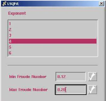
assuming the intercept on the Y axis is the appropriate form factor (1 + k) as illustrated in Figure 1. The default value for Fr power n is 4 however the user is encouraged to replot with other values of n and review the linearity and the sensitivity of the intercept (1 + k) to n. The value of n giving the best fit to the data is selected.
4.0 DESCRIPTION OF EXISTING IOT BARE HULL FORM FACTOR ANALYSIS SOFTWARE
The data acquired from standard calm water hull resistance experiments is normally used to derive the Prohaska form factor. IOT’s existing resistance analysis suite is described in detail on the IOT intranet home page (Reference 8). The display with the Prohaska form factor plot is shown in Figure 2. The user has the option of limiting the Froude Number range (normal range selected is 0.12<Fr<0.2) and choosing the Frn power in integer values from one to six (Figure 3). Once the range and Fr power has been selected, a linear polynomial is fit to the data and the intercept on the Y axis is
determined to be the Prohaska form factor (1+k). This value is stored in A2 of the main CFT point file to compute residuary resistance coefficient (CR) in the ITTC 1978
resistance analysis as described in Reference 4:
CR = CTM – (1 + k)*CFM (5)
5.0 APPLYING CHAUVENET’S CRITERION
From Reference 1, Chauvenet’s Criterion defines an acceptable scatter around a mean value from a given sample of N readings from the same parent population and is computed as follows:
τ = Xi – Xmean/SX (6)
Where:
τ - nondimensional deviation Xi - value of sample
Xmean – mean value of sample readings
SX – standard deviation of sample readings
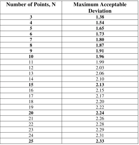
When applied to the Prohaska form factor situation, the criterion is used to assess maximum acceptable deviation from the mean line. Table 1 gives the maximum
acceptable deviation for a given sample size N where the numbers in bold are provided in the literature while the numbers in regular font are linearly interpolated values. The relationship between number of points (N) and maximum acceptable deviation is illustrated in Figure 4.
Chauvenet’s Criterion can be applied to the Prohaska form factor situation as follows: • Select Froude Number range – normal selected range is 0.12<Fr<0.20;
• Count the number of data points within the selected range to determine N; • Select Froude Number power n (Frn
) – the default for n is 4;
• Compute CTM/CFM for each data point in selected Froude Number range;
• Compute Frn
/CFM for each data point in selected Froude Number range;
• Evaluate value of slope of linear polynomial of CTM/CFM on Frn/CFM;
• Evaluate value of intercept on Y axis of linear polynomial of CTM/CFM on
Frn/CFM;
• Interpolate value of CTM/CFM on linear polynomial for each data point in selected
Froude Number range:
CTM/CFM(interpolated) = Frn/CFM* slope + intercept (7)
• Compute deviation from linear polynomial for each data point in selected Froude Number range:
Devi = (CTM/CFM(interpolated) - CTM/CFM) (8)
• Compute average value of all deviations from linear polynomial:
mean = Σ Devi/N (9)
• Compute standard deviation (st. dev.) of all deviations from linear polynomial: st. dev. = ((N*(Σ Devi2) – (Σ Devi)2)/N*(N - 1))1/2 (10)
• Compute Chauvenet’s Criterion nondimensional deviation value for each data point in selected Froude Number range:
ABS (Devi– mean)/st. dev (11)
If the Chauvenet’s Criterion nondimensional deviation value computed exceeds the Maximum Acceptable Deviation as specified in Table 1 for the number of data points within the selected Froude Number range, the point is identified as an outlier.
6.0 DISCUSSION 6.1 Chauvenet’ Criterion
Chauvenet’s Criterion was applied to the Prohaska form factor data from a number of model tests including:
• Great Lakes bulk carrier • Tanker
• Several competitive yacht hull forms at different heel angles
Very few outliers were identified using the criterion. An example Prohaska plot with an outlier that exceeds Chauvenet’s Criterion is provided in Figure 5 (form factor = 1.1475). The same plot with this single outlier removed is presented in Figure 6 (revised form factor = 1.1617). It is important to note that Chauvenet’s Criterion should only be applied to a given data set once. Thus once an outlier as determined by Chauvenet’s Criterion has been removed, the criterion is not applied to the same data set with reduced number of valid points (N) and a different value for the Maximum Acceptable Deviation. The advantage of applying a well known criterion to identify potential outliers is to provide some consistency to the overall data analysis. When the outliers are being
identified subjectively as is now the case, the analysis results may vary from user to user. An example of an auto scaled Prohaska Plot is provided in Figure 1. None of the points on this plot exceeded Chauvenet’s Criterion however some users may be tempted to remove some of the points since they ‘look bad’. The advantage of applying Chauvenet’s Criterion to the Prohaska plot algorithm is to provide some structured guidance to the user and some confidence in a consistent final data product.
6.2 Transom Stern Issues
It has been noted in several experiments carried out at IOT that there is a significant influence on the derivation of a Prohaska form factor of an immersed transom stern due to the added resistance increment resulting from flow separation off the transom edge at slow speed. An example yacht model Prohaska plot with transom stern immersed (form factor (1 + k) = 1.080) and without transom stern immersed (form factor (1 + k) = 1.035) is provided in Figure 7.
Where the transom is immersed only a few centimetres, transferring ballast forward to trim the model down by the bow without changing the overall displacement and executing a dedicated experiment to derive form factor may be a feasible option. For many common hull forms with transom sterns, however, such as a fully loaded Newfoundland fishing vessel or some modern patrol vessel designs, re-arranging the ballast to get the transom out of the water is not a feasible option due to the deep draft aft.
6.3 Influence of Appendages on Prohaska Form Factor
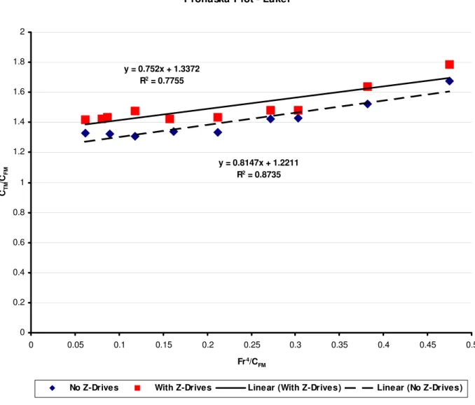
Acquiring resistance data over a low speed range (0.12<Fr<0.2) using a bare hull model fitted only with turbulence stimulators and appendages that are deemed to be part of the hull such as the a bulbous bow and skeg is the test method currently recommended by IOT (Reference 4) for deriving the bare hull Prohaska form factor. To reduce required resources and tank time, or when using an existing model, it is sometimes tempting to use resistance data from a partially appended model to derive the bare hull Prohaska form factor. The influence on derived Prohaska form factor for a large full form bulk carrier
fitted with faired dummy Z-drives (Figure 8) and without Z-drives for the same model displacement is illustrated in Figure 9. It is noted that with the addition of these simple faired appendages on a large model, the Prohaska form factor (1 + k) was increased from 1.221 to 1.337. The addition of an appendage of this type can have a significant
influence on form factor.
6.4 Deriving the Prohaska Form Factor on Full Hull Forms
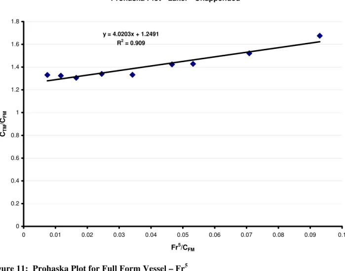
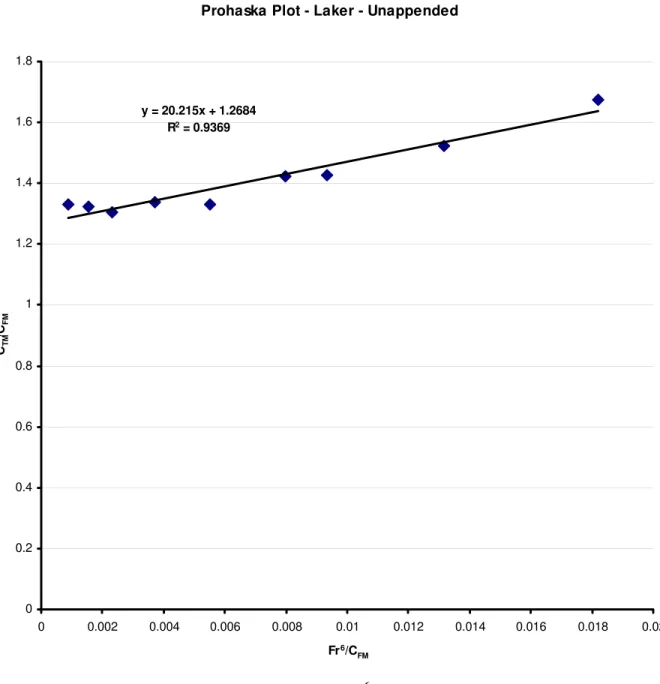
It is noted in Reference 7, pp. 103 that the normal Prohaska plot (CTM/CFM on Fr4/CFM)
can assume a concave shape using data acquired for vessels with block coefficients > 0.8. A Prohaska plot using Fr with a power between 4 and 6 is recommended. Prohaska plots for a Great Lakes bulk carrier with a block coefficient of 0.872 are presented in Figures 10 (Fr4), 11 (Fr5), 12 (Fr6), 13 (Fr8) and 14 (Fr10). Note that as the Frn power increases, the value of the form factor increases, the linear fit improves and the full scale effective power (PE) predicted using ITTC 1978 decreases:
Fr4: (1 + k) = 1.221 R2 = 0.8735 PE = 5580.9 kW
Fr5: (1 + k) = 1.249 R2 = 0.9090 PE = 5472.3 kW
Fr6: (1 + k) = 1.268 R2 = 0.9369 PE = 5405.2 kW
Fr8: (1 + k) = 1.294 R2 = 0.9717 PE = 5333.9 kW
Fr10: (1 + k) = 1.310 R2 = 0.9839 PE = 5258.0 kW
Thus it is apparent that varying the Frn power has a significant effect on overall resistance test results. Which result is correct? Without a correlation between an ITTC 1978 powering prediction and quality full scale trials data, it is impossible to say.
7.0 RECOMMENDATIONS 7.1 Chauvenet’ Criterion
It is recommended that Chauvenet’s Criterion as described in Section 5.0 be added to the Prohaska Plot algorithm in the IOT standard resistance analysis software to provide the user with some confidence in the integrity of the points. The Prohaska form factor data should be plotted as in Figure 1 and all data points that exceed the maximum acceptable deviation from the linear polynomial as determined using Chauvenet’s Criterion included on the plot but identified with a different symbol. The linear polynomial and form factor should be computed excluding these points. The number of points rejected using
Chauvenet’s Criterion should be displayed on the plot (if no points are rejected, this information should also be displayed on the plot) and the user given the option of
interactively retaining them and/or excluding others. All changes in the number of points retained should be reflected in an amended linear polynomial and amended computed form factor. A lookup table is recommended as the simplest and most accurate method of including the Maximum Acceptable Deviation (Table 1) in a resistance test analysis program.
It is also recommended that the following change be made to Sect. 4.5.4 the IOT Resistance Test Standard (Reference 4):
Change: ‘Due to the potential errors in measured resistance at low speeds, outlying points should be identified and excluded from the regression analysis.’
To: ‘Due to the potential errors in measured resistance at low speeds, outlying points as
determined using Chauvenet’s Criterion should be identified and excluded from the regression analysis.’
7.2 Transom Sterns
It is recommended that the experimentalist use some judgment when designing resistance experiments on vessels with transom stern arrangements. Where it is deemed feasible to re-arrange the ballast to elevate the transom clear of the water without changing the overall displacement, dedicated experiments over a Froude Number range of 0.12<Fr<0.2 should be carried out explicitly to derive an accurate Prohaska form factor. Where
experiments must be carried out with the transom immersed, the resistance and effective power should be computed using the ITTC 1957 ship-model correlation line without form factor.
It is also recommended that the following change be made to Sect. 4.5.4 the IOT Resistance Test Standard (Reference 4):
‘If feasible, the ballast on vessels with transom sterns should be re-arranged to ensure the transom is clear of the water during dedicated experiments to determine the Prohaska form factor. Where experiments must be carried out with the transom immersed, the resistance and effective power should be computed using the ITTC 1957 ship-model correlation line without form factor.’
7.3 Appended Models
Deriving the bare hull Prohaska form factor using a model fitted with appendages other than those appendages considered part of the hull as defined in Reference 4 is not recommended as the added resistance can significantly increase the form factor value. The method of deriving the impact on form factor due to the presence of appendages is described in Reference 4 and it is recommended that both bare hull and appended resistance experiments be carried out.
7.4 Full Hull Forms
IOT is committed to adhering to the recommendations of the ITTC with respect to carrying out standard model experiments. During the 23rd ITTC in 2002 (Reference 9), the derivation of the Prohaska form factor using a plot of CTM/CFM on Fr4/CFM was
confirmed. Although some sources (eg: Reference 7) recommend using a higher power for Fr and existing IOT software has the capability of applying a higher power, it is
recommended that IOT continue to adhere to the ITTC standard. If the Prohaska curve turns up at the low Fr4/CFM values, it may be an indication of flow separation due to the
bluff bow geometry. If this is the case, it is recommended in Reference 6 that these deviating data be omitted from the determination of 1 + k by increasing the lower limit of the selected Froude Number range. The authors of this report concur with that
recommendation.
There may be an opportunity in the future for IOT to take the lead in investigating these issues further and perhaps making a submission based on rigorously validated data to the ITTC Propulsion Committee for the benefit of the global ship model research
community.
8.0 ACKNOWLEDGEMENTS
The authors would like to thank Mr. D.C. Murdey for his input and advice on the issues discussed in this document.
9.0 REFERENCES
1) Coleman, H.W., Steele, Jr., W.G., ”Experimentation and Uncertainty Analysis for Engineers”, 2nd Edition, John Wiley & Sons, New York, 1999, p. 35.
2) Report of the Performance Committee, Proc. 15th ITTC, The Hague, 1978, pp. 388 – 392.
3) Recommendations of the Performance Committee, Proc. 16th ITTC, Leningrad, 1981, pp. 183.
4) Institute for Ocean Technology Standard Test Methods, Resistance in Open Water, TM-5.
5) Kiss, T.K., Compton, R.H., “ The Effects of Transom Geometry on the Resistance of Large Surface Combatants”, SNAME Transactions, Vol. 97, 1989, pp. 339-373.
6) Holtrop, J., ”Extrapolation of Propulsion Tests for Ships with Appendages and Complex Propulsors”, SNAME Marine Technology, Vol. 38, No. 3, July 2001, pp.145-157.
7) Harvald, SV., AA., “Resistance and Propulsion of Ships”, John Wiley & Sons, New York, 1983, p. 102.
8) IOT Resistance and Propulsion Software, http://odin/RSPWeb/RSPHome.asp, February 18, 2004.
9) Report of the 23rd ITTC Specialist Committee: Procedures for Resistance, Propulsion and Propeller Open Water Tests, Venice, Italy, September 2002.
Number of Points, N Maximum Acceptable Deviation 3 1.38 4 1.54 5 1.65 6 1.73 7 1.80 8 1.87 9 1.91 10 1.96 11 1.99 12 2.03 13 2.06 14 2.10 15 2.13 16 2.15 17 2.17 18 2.20 19 2.22 20 2.24 21 2.26 22 2.28 23 2.29 24 2.31 25 2.33
Figure 1: Typical Prohaska Form Factor Plot Output by IOT Standard Analysis Software
Figure 2: IOT Standard Resistance Analysis Software: Prohaska Form Factor
Figure 3: IOT Standard Resistance Analysis Software: Selection of Froude Number
Chauvenet's Criterion 0 0.5 1 1.5 2 2.5 0 5 10 15 20 25 Number of Points, N
Maximum Acceptable Criterion
Figure 4: Chauvenet’s Criterion: Relationship Between Number of Points N and Maximum Acceptable Criterion
Prohaska Plot - Yacht #3 - 25 deg. Heel Angle y = 0 .2 0 74 x + 1.14 75 R2 = 0 .70 58 1.08 1.10 1.12 1.14 1.16 1.18 1.20 1.22 1.24 1.26 1.28 0.00 0.10 0.20 0.30 0.40 0.50 0.60 Fr4/C FM CTM /C FM Outlier
Figure 5: Prohaska Plot with Identified Outlier
Prohaska Plot - Yacht #3 - 25 deg. Heel Angle
y = 0.1682x + 1.1617 R2 = 0.8364 1.08 1.10 1.12 1.14 1.16 1.18 1.20 1.22 1.24 1.26 1.28 0.00 0.10 0.20 0.30 0.40 0.50 0.60 Fr4/CFM CTM /C FM
Prohaska Plot - Yacht y = 0.1538x + 1.0351 R2 = 0.9504 y = 0.1564x + 1.0797 R2 = 0.9932 1.02 1.04 1.06 1.08 1.1 1.12 1.14 1.16 1.18 1.2 0 0.1 0.2 0.3 0.4 0.5 0.6 0.7 0.8 Fr4/CFM CTM /C FM
Figure 7: Prohaska Data With/Without Transom Stern Immersed Transom Immersed
Transom Immerged
Prohaska Plot - Laker y = 0.752x + 1.3372 R2 = 0.7755 y = 0.8147x + 1.2211 R2 = 0.8735 0 0.2 0.4 0.6 0.8 1 1.2 1.4 1.6 1.8 2 0 0.05 0.1 0.15 0.2 0.25 0.3 0.35 0.4 0.45 0.5 Fr4/C FM CTM /C FM
No Z-Drives With Z-Drives Linear (With Z-Drives) Linear (No Z-Drives)
Prohaska Plot - Laker - Unappended y = 0.8147x + 1.2211 R2 = 0.8735 0 0.2 0.4 0.6 0.8 1 1.2 1.4 1.6 1.8 0 0.05 0.1 0.15 0.2 0.25 0.3 0.35 0.4 0.45 0.5 Fr4/C FM CTM /C FM
Prohaska Plot - Laker - Unappended y = 4.0203x + 1.2491 R2 = 0.909 0 0.2 0.4 0.6 0.8 1 1.2 1.4 1.6 1.8 0 0.01 0.02 0.03 0.04 0.05 0.06 0.07 0.08 0.09 0.1 Fr5/CFM CTM /C FM
Prohaska Plot - Laker - Unappended y = 20.215x + 1.2684 R2 = 0.9369 0 0.2 0.4 0.6 0.8 1 1.2 1.4 1.6 1.8 0 0.002 0.004 0.006 0.008 0.01 0.012 0.014 0.016 0.018 0.02 Fr6/C FM CTM /C FM
Prohaska Plot - Laker - Unappended y = 523.09x + 1.2937 R2 = 0.9717 0 0.2 0.4 0.6 0.8 1 1.2 1.4 1.6 1.8
0.00E+00 1.00E-04 2.00E-04 3.00E-04 4.00E-04 5.00E-04 6.00E-04 7.00E-04 8.00E-04
Fr8/CFM
CTM
/C
FM
Prohaska Plot - Laker - Unappended y = 13652x + 1.3102 R2 = 0.9839 0 0.2 0.4 0.6 0.8 1 1.2 1.4 1.6 1.8
0.00E+00 5.00E-06 1.00E-05 1.50E-05 2.00E-05 2.50E-05 3.00E-05
Fr10/CFM CTM
/C
FM