Hydrodynamics in a stirred tank in the transitional flow regime

HAL Id: hal-01982666

https://hal.archives-ouvertes.fr/hal-01982666

Submitted on 15 Jan 2019

HAL is a multi-disciplinary open access

archive for the deposit and dissemination of

sci-entific research documents, whether they are

pub-lished or not. The documents may come from

teaching and research institutions in France or

abroad, or from public or private research centers.

L’archive ouverte pluridisciplinaire HAL, est

destinée au dépôt et à la diffusion de documents

scientifiques de niveau recherche, publiés ou non,

émanant des établissements d’enseignement et de

recherche français ou étrangers, des laboratoires

publics ou privés.

Hydrodynamics in a stirred tank in the transitional flow

regime

Freyman Mendoza, A. Lopes Bañales, Emmanuel Cid, Catherine Xuereb,

Martine Poux, David F. Fletcher, Joelle Aubin

To cite this version:

Freyman Mendoza, A. Lopes Bañales, Emmanuel Cid, Catherine Xuereb, Martine Poux, et al..

Hy-drodynamics in a stirred tank in the transitional flow regime. Chemical Engineering Research and

Design, Elsevier, 2018, 132, pp.865-880. �10.1016/j.cherd.2017.12.011�. �hal-01982666�

OATAO is an open access repository that collects the work of Toulouse

researchers and makes it freely available over the web where possible

Any correspondence concerning this service should be sent

to the repository administrator:

tech-oatao@listes-diff.inp-toulouse.fr

This is an author’s version published in:

http://oatao.univ-toulouse.fr/21125

To cite this version:

Mendoza, Freyman and Ba�ales, A. Lopes and Cid, Emmanuel and Xuereb,

Catherine and Poux, Martine and Fletcher, David F. and Aubin, Joelle

Hydrodynamics in a stirred tank in the transitional flow regime.

(2018) Chemical

Engineering Research and Design, 132. 865-880. ISSN 0263-8762

Hydrodynamics in a stirred tank in the transitional

flow regime

F.

Mendoza

a

_,

_A.

_{Lopes Baiiales}

a

_,

_{E. Cid}

a

_{, C.}

_Xuereb

a

_,

_M.

_Poux

a

_,

D.F.

Fletcher

b

_{,J. Aubin}

a

_,

_*

a Laboratoire de Génie Chimique, Université de Toulouse, CNRS, INPT, UPS, France

b School of Chemical and Biomo1ecu1ar Engineering, The University of Sydney, Australia

ARTICLE INFO

Keywords:

Mixing Stirred tank

Transitional flow regime CFD

PIV

Macro-instabilities

1. Introduction

ABSTRACT

The hydrodynamics in a stirred tank in the transitional flow regime have been studied experimentally and numerically with data obtained by Particle Image Velocimetry and Com­ putational Fluid Dynamics, respectively, at three Reynolds numbers, Re= 340, 980 and 3000. The effects of impeller rotation speed and fluid properties on the underlying flow struc­ tures have been investigated. Data are analysed by mean flow fields, as well as with Proper Orthogonal Decomposition, which gives an insight into the flow dynamics by separating the spatial and temporal characteristics of the flow structures. Experimentally, it has been found that dimensionless velocity fields depend on fluid properties and impeller speed at Re= 340 and 980, whilst they are self-similar at Re= 3000. Coherent flow structures only exist however at Re= 340 and the flow is structurally different than that at higher Re. Character­ istic frequencies identified for Re= 980 and 3000 are 0.03N and 0.13N, which are consistent with previous work in the literature. The simulations conducted at Re= 340 are in reasonable agreement with the experimental data, however, they do not predict a dependency of flow characteristics on fluid properties and impeller speed. This inconsistency is attributed to the difficulty of performing experiments that are free of physical perturbations, which may have a significant effect on flows at low transitional Reynolds numbers.

Whilst much research in the past two decades has focused on process intensification and new technologies for continuous processing, which demonstrate numerous advantages, traditional batch stirred tanks are still largely present in the process industries. Indeed, the replacement of existing batch processes with continuous flow technologies is not systematic mainly because companies do not want to, or cannot, rein­ vest in new equipment and process expertise, regardless if there could be significant gains in terms of product quality, productivity, safety and/or environmental impact. As a result, industry is still seeking to improve their understanding and engineering knowledge of existing batch processes and particularly how the process can be operated in order to contrai product quality, as well as to manage possible down­ stream processing steps, energy and waste.

Amongst the numerous batch stirred tank processes present in a broad range of sectors, including chemicals, agrochemicals, pharma­ ceuticals, cosmetics, food and mining, operation in the transitional flow regime is very frequent. This is mainly because in stirred tanks the laminar flow regime is limited to very low impeller Reynolds num­ bers (Re), typically Re< 10-100, the onset of flow instabilities occurring earlier than in tubes due to the rotating impeller and interaction with the vesse! geometry. The fully-developed turbulent flow regime is typ­ ically considered when Re:,. 20 000, although studies have shown that a Re:,. 300 000 is often required in order to obtain fully turbulent flow in bath the recirculation zone and the top third of the tank (Machado et al., 2013). Despite this, a large majority of studies presented in the literature dating back to the 1950s focus on full-developed turbulent flows or purely laminar flows. This is bec a use flow instabilities and the Jack of scaling of transitional flows make experiments and simulations

* Corresponding author.

E-mail address: joelle.aubincano@ensiacet.fr (J. Aubin). https:/ / doi.org/10.1016/j .cherd.2017 .12.011

difficult. As a result, engineering design rules and recommendations for stirred tank applications are typically valid for turbulent or laminar flows only.

The few studies in the literature dealing with the transitional flow regime in stirred tanks address specific particularities of these flows; however, determination of the general underlying reasons for physical phenomena occurring is not generally the focus. For example, Machado and Kresta (2013) and Machado et al. (2013) studied the transition from turbulent ta transitional flow in various stirred tank geometries in order ta determine the limits of fully turbulent scaling in different zones of the tank. They showed that although fully-developed turbulent flow is generally considered for Re> 20 000 in standard stirred tank geome­ tries, this is only true close ta the impeller. Reynolds numbers greater than 300 000 are required in order ta attain fully-developed turbulence at heights in the tank greater than 0.9T. However, in non-conventional geometries like the confined impeller stirred tank (CIST), fully turbulent flow was observed at Reynolds numbers as low as 3000. More generally, it was found that fully turbulent flow occurs at lower Reynolds num­ bers as the scale of the tank decreased and the ratio of impeller-to tank diameter DIT increased. They also showed that dimensionless veloc­ ity profiles at a fixed Reynolds number can depend on the viscosity of the Newtonian fluid, therefore affecting the flow regime in the tank. Liné et al. (2013) analysed the flow and the dissipation rate of a shear­ thinning liquid in the vicinity of a Rush ton turbine. Due ta the rheology of the fluid, the flow was expected ta be in the transitional flow regime with an impeller Reynolds of 530, determined using the Metzner-Otto carrela tian. However, the validity of this method and the spatial varia­ tion of the flow regime in the tank was not discussed. Recently, Alberini et al. (2017) have performed 3-dimensional Particle Tracking Veloci­ mentry (PTV) measurements in a stirred tank in transitional flow at Re= 70 and 1000 with the objective of comparing the measurement technique with 2-dimensional 2-component Particle Image Velocime­ try (PIV) for Newtonian and non-Newtonian flows. Although the work does not focus on the characteristics of transitional flow, the authors note a slight difference in the PTV and PIV velocity fields in the impeller discharge with non-Newtonian flow. This is attributed ta the unstable nature of transitional flow and suggests that the tangential velocity component may be of significance in such flows.

Other studies have been dedicated ta macro-instability phenomena occurring in stirred tanks in different flow regimes. Bruha et al. (1996) used a tornadometer ta determine the frequency of macro-instabilities (MI) as a fonction of Reynolds number for the range 210-67000. No insta­ bilities were observed when Re= 200, whilst a more or less constant frequency of 0.04N--0.05N was found for Re> 9000. For intermediate Re, however frequencies were found ta increase logarithmically with Re but no physical interpretation of the phenomena was provided. On the other hand, the same group of authors later reported a fre­ quency of 0.087N at Re= 750 and 1200 obtained with Laser Doppler Velocimetry (LDV) measurements (Montes et al., 1997). Galletti et al. (2004) further studied the effects of fluid properties, operating con­ ditions, as well as impeller and tank geometry on the frequencies of MI occurring from precessional vortex motion for Reynolds numbers ranging from 400 ta 54400. They made point measurements of the fluid velocity close ta the free liquid surface using LDV and found that for 400<Re<6300 the MI are characterised by a frequency of 0.106N, whilst in the range 13 600<Re<54 400, the frequency of 0.015N was dominant. In the intermediate range, however, bath frequencies were present. They also found in general that at constant Re, a change in fluid properties did not affect the characteristic frequency, although their results do show some dispersion at the lowest Reynolds num­ bers studied. Later, Ducci and Yianneskis (2007) and Ducci et al. (2008) focussed on the physical mechanisms underlying the precessional vor­ tex and associated frequencies. They conducted 2-dimensional velocity measurements on a horizontal plane under a Rushton turbine in the transitional regime 4400<Re<8000 and in turbulent flow, Re=27200 and analysed the data using Proper Orthogonal Decomposition (POO). They found that there are two mechanisms responsible for the MI vor­ tex. One is a perturbation that causes the vortex ta move off-centre and is related ta characteristic frequencies of 0.02N. The other is the elon­ gation of the vortex core, which is characterised by a frequency of 0.1N.

Their results show that the frequency 0.02N is associated with flows where Re> 6000. From the ensemble of these results, there appears ta be some clear trends on the formation and characteristics of vortex macro-instabilities at high transitional Reynolds numbers, i.e. Re> 4000 and valid mechanisms for the behaviour of the MI have been proposed. In the lower range of transitional Reynolds numbers, however, the con­ clusions are less explicit.

The simulation of transitional flows in stirred tanks is challeng­ ing because hydrodynamic instabilities create unsteady flow, which needs ta be correctly captured. Turbulence models are typically not well adapted at transitional flow Reynolds numbers because the eddy viscosity hypothesis used in the models is designed for high Reynolds number turbulence and also because the wall fonctions assume a log law at the wall. Ultimately, the full resolution of the time-dependent Navier-Stokes equations on an extremely fine 3-dimensional mesh would be desirable however such simulations require excessive com­ puting efforts, which may not be viable for practical engineering applications. As a result, there are very few studies in the literature that deal with the simulation of transitional flow in stirred tanks and almost ail of the available literature may be attributed ta a single author (Derksen, 2011, 2012a, 2012b, 2013; Zhang et al., 2017). In his studies, Derksen has used the Lattice Boltzmann method ta perform direct numerical simulations (ONS) of flows with Reynolds numbers in the range 2000-12000. These are extremely intensive computations, which require around 100 impeller revolutions on a highly-refined grid. Although these studies do not focus particularly on the underlying nature of the transitional flow, but rather specific mixing applications, the results demonstrate that moderate Reynolds numbers allow the flow ta be simulated directly, without the use of a turbulence clo­ sure or subgrid-scale models. Although, in their recent study, Zhang et al. (2017) have shown that even for simple Newtonian flows, ONS failed ta correctly predict the flow patterns and velocity fluctuation levels at certain transitional Reynolds numbers. Their work also shows the current state of confusion in modeling transitional flows as they attempted ta apply transition models developed for externat aerody­ namics ta internai flow and performed fini te volume simulations using 2nd order upwind differencing that they erroneously called finite vol­ ume ONS. The limits and capacities of simulation techniques (e.g. CFD, Lattice Boltzmann) for transitional flows in stirred tanks are therefore not clearly identified. Moreover, as various authors have discussed, the flow regime in a stirred vesse! is rarely constant in the entire volume (Ducci et al. 2008; Machado et al. 2013); in some cases, flow may be fully turbulent in the vicinity of the impeller but in the transitional or even laminar flow regime in zones further away. It is not straightforward ta know how this variation in flow regime should be taken into account in simulations that can be performed with reasonable computational effort and therefore applicable for engineering applications.

The global objective of this work is ta con tribu te the knowledge of transitional flows in stirred tanks in order ta develop engineering guide­ lines and tools that will ultimately lead ta increased process/product understanding and improved product development and manufactur­ ing. In particular, this study aims at exploring the effects of Newtonian fluid properties (viscosity, density) and impeller rotation speed on the characteristics of transitional flow experimentally via PIV measure­ ments and numerically with transient laminar flow CFD simulations. The flow is examined using conventional mean flow analysis and the in more detail with POO.

2. Materials and methods

2.1. Stirred

tank

geometry

The tank geometry employed in this work is a dish-bottomed cylindrical tank, T= H = 0.19 m, with four equally spaced Per­ spex baffles of width w=T/10 placed 90° to each other. The cylindrical vessel is placed inside a square tank whose front panel is transparent to allow distortion-free velocity mea­ surements. The tank was filled with plain water and is

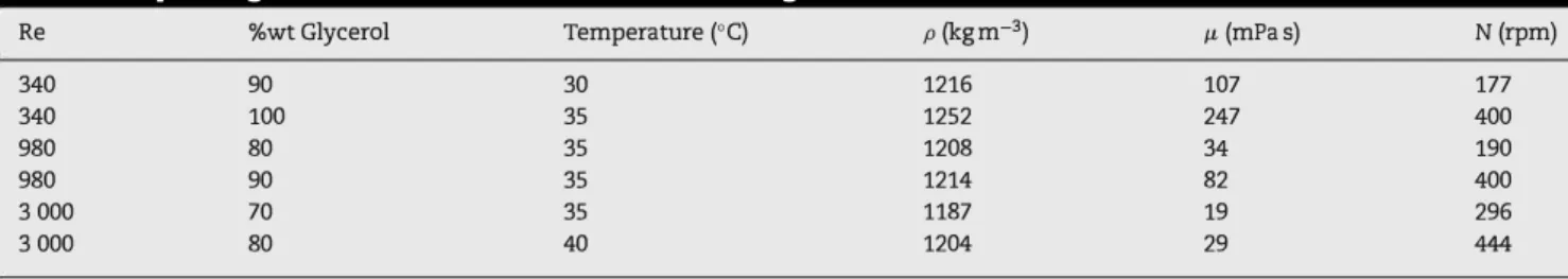
Table 1 - Operating conditions for the different cases investigated. Re %wt Glycerol Temperature ('C) 340 90 30 340 100 35 980 80 35 980 90 35 3 000 70 35 3 000 80 40

connected to a pump and a heating element in order to heat the working fluid in the cylindrical tank to a specific temperature. The cylindrical tank is equipped with a down­ pumping Lightnin A320 axial flow impeller (D = T/2), which is a wide-bladed hydrofoil impeller that is recommend for higher viscosity applications and low Reynolds number. The impeller is mounted on a shaft, s = 0.008 m, which extends to the bot­ tom of the vesse!. The impeller clearance is C = T/3, where C is defined as the distance from the vesse! bottom to the lowest horizontal plane swept by the impeller.

2.2. Operating conditions

The operating conditions were chosen to obtain two experi­ mental datasets for three different Reynolds numbers equal to 340, 980 and 3000. To do this bath the fluid viscosity, /t, and the impeller speed, N, were varied. To vary the fluid viscosity dif­ ferent concentrations of aqueous glycerol solutions were used at different temperatures. Temperature controlled viscosity measurements were made with an AR 2000 rheometer (TA Instruments); density was measured with a DMA 38 densime­ ter (Anton Paar) where temperature is controlled with a Peltier resistance. Care was taken to keep the axial impeller tip speed (:rrND) in the recommended range of 1-5 m s-1. Table 1 shows the operating conditions for the six different cases studied. 2.3. Partide image velocity

measurements

Full field 2-dimensional, 2-component velocity measurements encompassing almost the entire height of the tank (except for in the dished-bottom) were performed using PIV. The PIV was composed of a double pulsed Nd:YAG laser (532 nm, 2 x 120 mJ, Nanopiv - Litron Lasers). The liquid was seeded using rhodamine-doped polymer particles (dp = 10-30 µm)

(microParticles GmbH, Germany). A black and white CCD cam­ era (ImagerProPlus) with a resolution of 4032 x 2688 pixels2

and a high-pass filter was used to record instantaneous images of the flow in a plane midway between two baffles. Image pairs were taken at a rate of 9 Hz and for each case 1000 instantaneous velocity fields were recorded. These images were processed using DaVis software (LaVision, Germany). A decreasing interrogation window size (from 64 x 64 pixels2

to 32 x 32 pixels2) _{with 50% overlap and the standard cross­}

correlation with Fast Fourier Transform (FFT) was used to determine the corresponding spatially averaged displacement vectors. The spatial resolution was 1.5 mm.

2.4. CFD simulations

Transient, laminar flow simulations for bath cases at Re= 340 were made using the commercial CFD software ANSYS CFX (V18.1). A CAO model of the A320 impeller supplied by SPXFLOW was de-featured and incorporated into a mode!

p (kgm-3) µ, (mPas) N(rpm) 1216 107 177 1252 247 400 1208 34 190 1214 82 400 1187 19 296 1204 29 444

of the vesse! using ANSYS SpaceC!aim. A tetrahedral mesh, with 5 layers of inflation at the walls, was then created with three different mesh densities, comprising 1.01, 2.07 and 6.46 million cells. Ali presented simulation results used the finest mesh (see later for details). The equations were solved using the coupled solver with High Resolution differencing for the convective terms and the Second Ortler Backward Euler scheme for the time derivatives. The solution at any time­ step was deemed to have converged when the normalised RMS residuals fell below 10-5.

Initially a steady-state simulation was run using the Frozen Rotor model, which assumes fixed relative position of the blades and baffles, to generate a starting flow and to study mesh dependency. Following this, transient simulations were run using the moving mesh approach with the Transient Rotor Stator interface model and a 2° _{displacement of the}

blades per time-step. Simulations were continued for over 200 revolutions of the impeller in bath cases. At these times, quasi­ periodic behaviour of the torque on the blades was observed. Data generated only after the quasi-periodic behaviour was established were used in the flow analysis. Velocity data were output on a vertical plane midway between the baffles every 0.022 s (45 Hz sampling frequency), which is 5 times that used in the experiments (9 Hz). The high sampling frequency allows numerical data to be analysed at either 9 Hz or 45 Hz, thereby allowing the effect of the sampling frequency on the results to be studied. In bath cases, however, the number of data fields used for the analysis spans 62 impeller revolutions, which is much longer than the period of the flow structures being detected.

2.4.1. Computational setup and mesh

The geometry together with the location of the rotating zone (grey) and the sampling plane (red) are shown in Fig. 1(a). The vertical sampling plane is positioned midway between two baffles and extends from the shaft to the tank wall. This fig­ ure also shows the computational mesh on the impeller for the 6.46 million element mesh. The top of the vesse! (green) coïncides with the mean liquid level, which was assumed to be fiat, and a no stress boundary condition was applied. A cross­ section of the 6.46 million element mesh in the en tire tank is given Fig. 1(b).

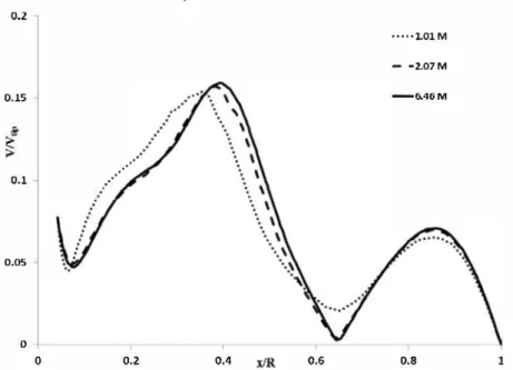
As mentioned above, steady-state Frozen Rotor simula­ tions were run on three different mesh densities. In order to access mesh dependency effects, the velocity magnitude was extracted on a horizontal line from the tank centre to the wall at three-quarters height and compared for the three mesh densities. The results, given in Fig. 2, show that there is a significant difference between the coarse and medium meshes but only a small difference when the medium and fine meshes are compared. Given the simulation times were acceptable, typically taking 40 min per revolution on 24 cores, ail simulations used the finest mesh.

Fig. 1 - Geometry (a) and mesh (b) used in the simulations of the fully baffled dish-bottomed tank with A320 impeller. (For interpretation of the references to colour in the text, the reader is referred to the web version of this article.)

0.2 •• .. •LOl M - •2.07M 0.15 -6.46M 0.1

.···

0.05 0 0 0.2 0.4 0.6 0.8 l

Fig. 2 - Normalized velocity magnitude on a horizontal line located on the sampling plane at three quarters of the vessel height.

2.5. Proper Orthogonal Decomposition technique

Proper Orthogonal Oecomposition (also known as Karhunen-Loève decomposition in signal processing and principal component analysis in statistics) is a data processing technique, which enables large amounts of high-dimensional data to be transformed into simpler, lower-dimensional data sets that capture the key phenomena. In fluid mechanics, POO is known to be an efficient tool for isolating coherent structures from a series of instantaneous velocity fields in complex flows, as well as understanding their dynamics and predicting their temporal evolution (Holmes et al. 1997).

POO is a linear procedure, which decomposes a set of instantaneous velocity fields into a modal base, thereby allow­ ing organized motion to be distinguished from turbulent motion (Berkooz et al., 1993). The different modes are ordered in terms of their contribution to the total kinetic energy in the plane of measurement, with the first mode being the most energetic and the last the least energetic. In this work, POO is implemented via the 'snapshot method' and is used to identify

coherent structures in the flow and to characterize the sensi­ tivity of the flow structures to changes in fluid properties and operating conditions.

2.5.1. Snapshot method

In this section, a brief description of the snapshot method is given; for a more detailed description, the reader is referred to the founding works of Sirovich (1987) and Berkooz et al.

(1993). The reader is also referred to the works of Liné et al.

2013 and Oucci et al. 2008 for the specific mathematical details

of the snapshot method applied to PIV data. In this work, n instantaneous velocity fields in the X-Z plane are obtained by either PIV and CFO and each instantaneous velocity field measurement constitutes a snapshot of the flow dynamics.

Eq. (1) describes the POO analysis applied to the fluctuating part of a measured velocity field, where

"i.\

and Vmean are the

total and mean velocity flow fields, respectively. For each mode I, the POO method generates 'P(I) and ai).

The variable 'P(I) is the spatial eigenfunction of mode I and is independent of time, or the instantaneous event, k. The

vari-able ail is the instantaneous temporal coefficient of mode I that is spatially independent; it also controls the importance of the eigenfunctions and the way they contribute in time to the total flow.

n

- - _{'"""(!) -(!)} Vk (x, y, z, t) = Vmean (x, y, z, t) + � ak (t) q., (x, y, z)

1�1 (1)

The spatial eigenfunctions <p(I) are orthogonal to each other while the temporal coefficients ail (t) are uncorrelated in time. The spatial eigenfunctions are obtained from the eigenmodes of the two-point correlation tensor, C, as given in Eq. (2).

(2) where ;..(!_{) is the eigenvalue, which represents the energy con­}

tent associated with eigenfunction <p(I) and its contribution to the total kinetic energy. The correlation tensor, or auto­ covariance tensor, is given by Eq. (3).

C = Vi (x, y, z, t)

.V

_j (x, y, z, t)

(3)

where the indices i and j refer to different points in the grid of measurements. It is worth noticing that numerically the auto-covariance tensor can also be given by Eq. (4).

... w'(x,,J

(4)

where M is the snapshot matrix, which is composed of the entire data set of instantaneous velocity fields. Each instan­ taneous velocity field is disposed in the matrix as a column vector, with the axial component u1 and the radial compo­ nent w1 of velocity in the same matrix column, followed by the next instantaneous velocity field in the next column and so on for n snapshots, as shown in Eq. (5).

(5)

Finally, the POD coefficients ail (t) are obtained by project­ ing each instantaneous velocity field on the I-th eigenfunction, <p(I) as given in Eq. (6).

3. Results and discussion

3.1.

Experimental data

3.1.1.

Mean flow

(6)

For each Reynolds number, the mean velocity field is cal­ culated as the time average of the entire dataset, which is composed of n = 1000 instantaneous velocity fields. The velocity components are normalized by the tip speed of the impeller, Vtip· Normalised axial velocity component profiles are also plotted at three different heights in the tank: h = 0.29H, immediately below the impeller swept plane; h=0.5H, mid­ height of the tank; h = 0.75H in the upper part of the tank.

Figs. 3-5 show the mean velocity fields for two different sets

of operating conditions at Re= 340, 980 and 3 000, respectively.

The line between y/H = 0 and y/H = 0.2 depicts the dished bot­ tom of the tank where no measurements were taken. These figures show the presence of a single circulation loop in the lower half of the tank that is characteristic of an axial flow impeller. In a general manner, as the Reynolds decreases the size of the circulations decreases and the jet expelled from the impeller-swept volume has an increasingly impor­ tant radial flow component to it. This is expected behaviour as it is well known that the pumping capacity of axial flow impellers decreases as the flow becomes laminar (Hemrajani

and Tatterson, 2004).

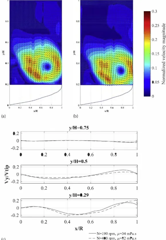
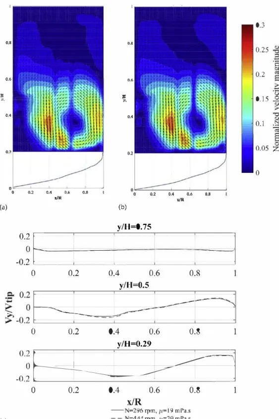
Comparing Fig. 3(a) and (b), it can be seen that the circu­ lation loop is slightly smaller with the lower values of fluid viscosity and impeller speed, but the maximum relative veloc­ ity is slightly higher. Indeed, the normalised axial velocity component profiles taken at different heights in the tank, shown in Fig. 3(c), do not collapse (particularly close to the impeller swept zone), which is usually the case for highly laminar and fully-developed turbulent flow. In the upper part of the tank, the fluid velocity is close to zero. When the Reynolds number is increased to 980, as shown in Fig. 4, the flow patterns and velocity magnitudes are qualitatively similar when there is a change in impeller speed and fluid viscosity, however comparison of the axial velocity compo­ nent profiles still reveals a lack of self-similarity. Increasing the Reynolds number further to 3000, as shown in Fig. 5, results in mean velocity fields around the impeller that are inde­ pendent of impeller speed and fluid viscosity, as would be expected for turbulent flow. However, although self-similarity is achieved at this Reynolds number in the vicinity of the impeller, fully-developed turbulent flow in the entire tank is not yet achieved. Indeed, the fluid velocity in the top third of the tank is very low so laminar flow would dominate in this zone. Using the relationship determined by Machado et al.

(2013), the dimensionless height, y/H, at which turbulent flow

should be achieved is 0.65. This is roughly the height at which the velocity magnitude is almost zero in Fig. 5.

3.1.2. POD eigenualue spectra

Fig. 6 shows the eigenvalue spectrum for the case with dif­

ferent Reynolds number equal to 340, 980, and 3000. This corresponds to the energy contribution of each mode to the total kinetic energy of the system. According to the energy cascade theory, the lower modes (denoted as eigenvalue num­ bers in Fig. 6) are typically associated with large scale flow structures, such as trailing vortices and macro-instabilities, whilst the higher modes are related to smaller scale flow structures and turbulence. When two consecutive modes have similar contributions to the total energy, they may reveal large scale coherent structures, i.e. large scale flow patterns that are organised and persistent as opposed to occurring randomly

(Moreau and Liné, 2006; Gabelle et al., 2013).

It can be seen in Fig. 6 that the energy contribution of the first mode generally decreases from about 18% to about 5% as the Reynolds number increases from Re= 340 to 3000. This is expected since as the Reynolds number increases, energy is dissipated down to smaller scales in the flow. It is also observed that at Re= 340, the impeller speed and fluid viscosity modify the eigenvalue spectrum. The modes associated with the large-scale flow structures have a greater contribution to the total energy in the flow when the impeller speed and fluid viscosity are low, whilst there is a higher energy contribution of the small-scale structures when the impeller speed and vis­ cosity are high. This result suggests that the impeller speed,

0.3

0.8

0.25

.":= O.G

0.2

.":::

0.15

0.4

0

.

1

N 0.2

0.05

0

0.8 0.2 0.4 0.(, 0.8 x/R x/R (a) (b)

y/H

=

0.75

O

.�

f

-0.2

• •

l

0

0.2

0.4

0.6

0.8

1

y/H=0.5

0.2

0.4

0.6

_0.8

1

y/H=0.29

0

_0.2

0.4

x/R

(c)

0.6

0.8

= 177 rpm, µ= _{l 07 mPa.s} =400 rpm, µ=247 ml>_{a_s}

1

Fig. 3 - Mean velocity fields at Re= 340. (a) N = 177 rpm and µ. = 107 mPa s; (b) N = 400 rpm and µ. = 247 mPa s; (c) comparison of normalized axial velocity profiles for both operating conditions.

and therefore inertia, is controlling the development of large­ scale flow structures rather than the viscous effects, as would be expected. As Re increases, however the effect of the oper­ ating conditions on the eigenvalue spectra diminishes, which means that the flow structures are becoming similar in terms of energy distribution.

3.1.3. POD spatial eigenfunctions

As mentioned in Liang & Dong {2015), POD is a possible method for decoupling spatial coherent structures from tem­ poral variations. The spatial structures, or eigenfunctions, are

presented in this section and their time-dependent behaviour determined from the time coefficients, a�!) (t) , in the next sec­ tion. It should be noted that the spatial structures do not correspond to velocity fields of actual vortices, but they give a qualitative sense of the type of structure that occur in the flow dynamics.

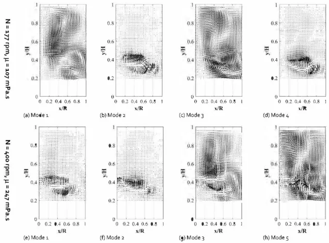
Figs. 7-9 show four spatial eigenfunctions for each of the

cases at Re= 340, 980 and 3000. At Re= 340, it is observed that when N = 177 rpm the flow structures represented by modes 1 and 3 occupy the entire mid plane of the tank, whilst for modes 2 and 4 they are limited to the vicinity of the impeller. In

0.3

0.8

0.25

-�

0.6

0.2

.f'

0.15

0.4

0.1

N 0,2

0.05

Z

.

0 0 0 0.2 0.4 0.6 0.8 _0.2 0.4 0.6 0.8 x/R x/R

{a)

(b)

y

/H

=

0.75

0.2

0

-0.2

0

0.2

0.4

0.6

0.8

1

y/H=0.5

.S< 0.

2

>

0

>

-0.2

0

_0.2

_0.4

_0.6

_0.8

y/H=0.29

(c)

0.2

0

-0.2

0

0.2

0.4

0.6

0.8

1

x/R

--N=l90 rpm, µ=34 mPa.s - - N=400 rpm, µ.=82 mPa.s

Fig. 4 - Mean velocity fields at Re= 980. (a) N = 190 rpm and µ. = 34 mPa s; (b) N = 400 rpm and µ. = 82 mPa s; (c) comparison of normalized axial velocity profiles for both operating conditions.

contrast, when N = 400 rpm, the structures depicted by modes 1 and 2 are restricted to a zone close to the impeller and modes 3 and 5 occupy the entire mid plane of the tank. It can also be seen that mode 1 at N = 177 rpm (Fig. 7(a)) is structurally similar to mode 3 at N = 400 rpm (Fig. 7(g)), and likewise for mode 3 at N = 177 rpm and mode 5 at N = 400 rpm. Note that no significant structures were present in modes 5 and 6 at N = 177 rpm or modes 4 and 6 at N = 400 rpm. It is noted that for bath operating conditions at Re= 340 the modes appear to be 'shuffled'; one would expect similar flow structures to be in consecutive pairs and the larger structures to have the highest

eigenvalues (as seen later in the CFD data). The origin of this 'shuffling' of the modes is not clear at this stage.

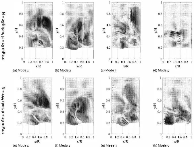
At Re= 980 and 3000 (Figs. 8 and 9), it can be seen that all of the flow structures in the first four to five modes fill most of the plane and that there are no structures that are only located in the vicinity of the impeller. It is also observed that at Re= 980, the structures in modes 1 and 2 are hardly affected by the operating conditions. This suggests that there is almost no difference in the macro flow dynamics because its two most energetic flow structures are very similar.

Sim-0.3

0.8

0.25

ï:

0.6 0.6

0.2

lC _:c "";.. _,:.

0.15

'û

0.4 _0.4 0.1

-�

0.2

0.05

z

0

0.2 0.4 0.6 0.8 _{0.2 0.4 0.6 0.8} ,c/R _x/R (a) (b)

y/H=0.75

0.2�

l

l

-0-�

-

1

-'-0

0.2

0.4

0.6

0.8

y/H=0.5

0

0.2

0.4

0.6

0.8

1

y/H=0.29

0.2

�.

o

�

-0.2

1

0

0.2

0.4

0.6

0.8

1

x/R

(c) -296 rpm, µ-19 mra.s =444 rpm, µ=29 mPa.s

Fig. 5 - Mean velocity fields at Re=3000. (a) N=296rpm andµ. =19mPas; (b) N=431 rpm and µ.=28mPas; (c) comparison of n ormalized axial velocity profiles for both operatin g cond itions.

ilarly, at Re= 3000, the flow structures for modes 1-3 appear ta be independent of the operating conditions. It is therefore possible ta deduce that as the Reynolds number increases, the dynamics of the flow becomes more robust and less sensitive ta changes in impeller speed and fluid properties.

3.1.4. POD time coefficients

The POD methodology not only provides information on the spatial structures in a flow, it also allows a temporal analysis of the flow structures. The time coefficients obtained by POD may be considered as weights, which are assigned ta the

instanta-neous velocity fields, providing information on the fraction of mode I that is contained in the instantaneous velocity field i. Analyses of the time coefficients - e.g. via phase portraits and Fast Fourier Transforms - enable one ta determine if two spatial modes are related and if they contribute ta coherent structures, or if there are dominant frequencies occurring in the flow.

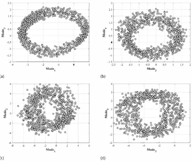
3.1.4.1. Phase portrait. Fig. 10 shows phase portraits, where the time coefficients for two spatial modes are plotted against one another, for Re= 340 for the two different operating

con-1d' 10·:l�---- ---lO" 101 _{10: ro-1} tli;rnvah,c- n11mh1:r {a) io-1

,--

---

-

...----

-

�

-

_

-

_

..,.

_

-

_

-

_

-

�

-

-

�

-

-

-

-�-=: ....

9 10-'

0 11=_{1!i2. mP.u...s, N=40fJ rpru}

c µ-3,4 mJ'l';u, 1"-190 rp-10 10·•------�-----�---- -IO" 101 _{ia' 10'} Eigenvalue number {b)

" "

..

,_

_{= "}

w'

�10·' 0 D 0 □ r.r=19 m.P!.,:, N=J.4-l rpm 1 1rl9 mr:t,s, N=296rpm 10-' ---�---�----� 10° 10' 10' 103 Eigenvalue number {c)

Fig. 6 - Eigenvalue spectra extracted from the experimental data. (a) Re= 340, (b) Re= 980, (c) Re= 3000.

<litions. The circular or elliptical shape of the phase portrait implies that there is a periodic relationship between the two modes and that they make a coherent structure. Note that two consecutive modes are not necessarily plotted together here since the ordering of modes is somewhat shuffled due as discussed in the previous section. In the low impeller speed and viscosity case, Fig. 10(a) and (b), modes 1 and 3 are coupled and modes 2 and 4 are coupled. Indeed, as seen

in Fig. 7, the spatial structures of modes 1 and 3 are simi­

lar in the fact that they fill the 2-dimensional measurement plane, and likewise for modes 2 and 4, where the spatial struc­ tures are limited to the zone around the impeller. Similar observations can be made for the case where N = 400 rpm and Il= 247 mPa S.

At Re= 980 and 3000, however, the phase portraits did not reveal the existence of any periodic coherent structures, at least not in the large plane of measurement considered in this work. Nevertheless, it is possible that in a smaller zone of mea­ surement, e.g. an are a restricted to the vicinity of the impeller, coherent structures may be found.

3.1.4.2. Analysis

of frequencies.

The time coefficients estab­ lish a spatial-temporal relationship between the eigenfunc­ tions and the instantaneous velocity fields that represent the temporal evolution of the different modes. As a consequence, it is possible to obtain the power spectrum of a mode by per­ forming a Fast Fourier transformation of the corresponding sequence of time coefficients. Fig. 11 shows the power spec­ tra associated with the spatial modes given in Fig. 7 that have been determined by FFT of the associated time coefficients. For the low impeller speed and viscosity case (Fig. 11(a)-(d)), it is not surprising to see that mode pairs associated with coherent structures, i.e. modes 1 and 3, and modes 2 and 4, have the same dominant frequency, 0.14N and 0.08N, respec­ tively. A similar observation is made for the higher impeller speed and viscosity case, where modes 1 and 2, and modes 3 and 5 have the same dominant frequencies of 0.31N and 0.16N, respectively. It is interesting to point out that although the space filling structures have similar frequencies regard­ less of the operating conditions (compare Fig. 11(a) and (c) where f=0.14N and Fig. 11(g) and (h) where f=0.16N), the

fre-z

Il

...

... ...

-a

}

1= Il

...

0 ... 3 "'tl Ill i,,

z

Il

�

₀ 0 l= Il tJ

�

... 3 "'tl Ill i,,

o����-�

0 0.2 0.4 0.6 0.8 1 x/R (a) Mode 1 0.8 · .:::::::::;::::::::::: _{... -} ., .. -... ,--·· ··-...

---�.:: l111:l1iil,li'I,

0.2 .. ""c;:::::c::c;:c: ... . 0 0 0.2 0.4 0.6 0.8 1 x/R (e) Mode 1 0.8 . :: 0.6

� .. "E,

_0.2

■

w1

o

������

0 0.2 0.4 0.6 0.8 1 x/R (b) Mode 2 0.8 _{·. :::::::c:. :}·:.

� ::rii!�i!!t

01

_{0 0.2 0.4 0.6 0.8 1} x/R (f) Mode 2

o

�-���

�

0 0.2 0.4 0.6 0.8 1 x/R (c) Mode 3 0 0 0.2 0.4 0.6 0.8 1 x/R (g) Mode 3 0.6. 0.4. 0.2

o��-���

0 0.2 0.4 0 6 0.8 1 x/R (d) Mode 4

o

�

0 0.2 0.4 0.6 0.8 1 x/R (h) Mode 5

Fig. 7 - Spatial eigenfunctions for Re= 340. (a)-(d) correspond to N = 177 rpm and /L = 107 mPa s. (e)-(h) correspond to

N = 400 rpm and /L = 247 mPa s.

z

Il

...

\D 0

...

"O 1= Il

...,

3 "'tl Ill i,,

z

Il

�

₀ 0

...

"O

�

3

l=

Il 00 tJ

3

"'tl Ill i,,

o

�-��

� �

0 0.2 0.4 0.6 0.8 1 .t/R (a) Mode 1 0.8

0

1

_{0 0.2 0.4 0.6 0.8 1} x/R (e) Mode 1 0.6

�

0.4 0.2 0 0 0.2 0.4 0.6 0.8 1 x/R (b) Mode 2 0.2 - : 0 0 0.2 0.4 0.6 0.8 1 x/R (f) Mode 2

-:;:::::

:·::·:::::::;;::·

o

�-�

�

��

0 0.2 0.4 0.6 0.8 1 x/R (c) Mode 3 il.-:<"::::

:i::::)i:::::; ,:::;::(

0 0 0.2 0.4 0.6 0.8 1 x/R (g) Mode4 0.8

_··---·

0.6 0.2

o

�

-

��

��

0 0.2 0.4 0.6 0.8 1 x/R (dl Mode 4 0 0 0.2 0.4 0.6 0.8 1 x/R (hl Modes

Fig. 8 - Spatial eigenfunctions for Re= 980. (a)-(d) correspond to N = 190 rpm and /L = 34 mPa s. (e}-(h) correspond to

Il

.. 3

1=

Il t,.I y:,

3

"'tl !1.1

"'

o���--��

0 0.2 0.4 0.6 0.8 x/R (a) Mode 1

o���-���

0 0.2 0.4 0.6 0.8 x/R (el Mode :i.

o

�

�

� -

�

�

�

0 0.2 0.4 0.6 0.8 x/R (b) Mode 2 0.6

o�-�--��

0 0.2 0.4 0.6 0.8 x/R (f) Mode 2

-

·

-

-

·=:

:

:

'

�:<:=:::::::

::,,

,1

0. 8 1

li,

lm

lU,t,11r ..

0.6 ' :

:fü'' '\,,

�: :

ll

!f

f

i

l

l

ll(

im�f �/li

_l

o

·�

�

� -

���

j

0 0.2 0.4 0.6 0.8 x/R (c) Mode 3

o���--��

0 0.2 0.4 0.6 0.8 x/R (g) Mode 3

o���-�-

�

0 0.2 0.4 0.6 0.8 x/R (d) Mode 4

o���-���

0 0.2 0.4 0.6 0.8 x/R (h) Mode 5

Fig. 9 - Spatial eigenfunctions for Re= 3000. (a)-(d) correspond to N = 296 rpm and IL= 19 mPa s. (e}-{h) correspond to N = 444 rpm and IL= 29 mPa s.

quencies of the structures that are restricted to the impeller zone are clearly dependent on the operating conditions. The frequency of these structures obtained with N = 400 rpm and 1-l = 247 mPa s is almost four times that for the case where N = 177 rpm and 1-l = 107 mPa s. A further difference in the two operating conditions is the existence of a secondary frequency in mode 1 and mode 3 for the high impeller speed and viscos­ ity case that is equal to the dominant frequency of mode 3 and mode 1, respectively. The origin of the se different frequencies, which depend on the operating conditions, is not entirely clear from the results presented here. In order better understand the trends of the observed frequencies and to correlate them with the underlying flow structures, a larger campaign of mea­ surements at low Reynolds number and with varying impeller speed and fluid viscosity would be required.

At Re è". 980, the characteristic frequencies become less dominant since coherent structures in the flow are absent. Nevertheless, prevailing frequencies can still be identified.

Table 2 shows the frequencies identified for the first and sec­

ond modes at the different operating conditions and Re= 340, 980 and 3000. It can be seen that the frequency identified for the first mode at Re= 980 and 3000 is 0.03N, which is an order of magnitude lower than the values obtained at Re= 340. The fre­ quency of the second mode, however, is around 0.12N, except for the low impeller speed and viscosity case at Re= 3000 where the value is 0.02N. It is interesting to point out that the frequencies identified for the cases where Re è". 980 are very similar to those identified for the precessing vortex macro­ instability at transitional flow Reynolds numbers by Galletti

et al. (2004) and Ducci et al. (2008). They identified two

fre-quencies: one at 0.02N, which was attributed to the off-centred precession of the vortex core, and the other 0.1N, which was related to the elongation of the vortex core and its rotation around its own axis. They found that as Re increases, the low frequency 0.02N peak is associated with the most energetic modes. Indeed, the results of this study for Re è". 980 show low frequency for mode 1 and high frequency for mode 2, except for the case at Re= 3000 with low impeller speed and viscos­ ity where the low frequency prevails in mode 2. The similarity of these results with those of Galletti et al. (2004) and Ducci

et al. (2008) strongly suggests that the instabilities detected

here are related to the vortex, which may be described as a large coherent structure that is convected by the mean flow

(Kresta and Roussinova, 2004). There is clearly a significant

difference in the behaviour of the flow structures at Re è". 980 and at Re< 980. At Re< 980, the frequencies depend strongly on the operating conditions and fluid properties, whilst at Re è". 980 the frequencies are quasi-independent of fluid prop­ erties, which is in agreement with Galletti et al. (2004). Note that although there appears to be an effect of the impeller speed and viscosity on the frequency of mode 2 at Re= 3000, it is pointed out that the frequency of mode 3 is 0.12N for the low viscosity case and 0.03N for the high viscosity case. Consider­ ing experimental error and consequent shuffling of modes, it can be considered that there is little effect of operating con­ ditions on the flow at Re= 3000. Furthermore, the appearance of the low frequency (0.02N) in the lower modes suggests that as the Reynolds number increases, the off-centred precession of the vortex core domina tes, as observed in previous studies

2.5 2 1.5 -j

-..,

0.5 -() --0,5 --1 --1.5 -2 -4 -3 -2 -1 0 Mode₁ (a) 6 4 -2 ( ) f 0

�·

2 --4 -6 -8 -6 -4 -2 0 2 4 Modc₁ (c) (b) 6 (d) r 2.5 2 1.5 11.5 0 -0.5 -1 -1.5 -2.5 -2 -1.S 4 -1 -0,5 0 J\llode₂ 0.5

,

---,

1.5 2 -3 '---��--�---�---�---� -8 -6 -4 -2 Modc3 0

Fig. 10 - Phase portrait of coefficients for Re= 340. (a), {b) correspond to N = 177 rpm and µ, = 107 mPa s. (c), (d) correspond to

N = 400 rpm and µ, = 247 mPa s.

,

,

I

l

I

_{,.,- I '}

_,

l'i, _., . ./ \ .. _. .. ..., Q '----=--c������----' (1 p ,14 116 {18 1 t'S (a) Mode 1 2.5 0.1 U.2 [1.3 O . .+ ,,...-; (e) Mode 1 IJ 1-1 16 o..: Q.6 U.7 (b)Mode 2 2.5 11

Il

Il

11 1..: 1 n ;, 1 1, . U �/ � --,,,• "'I _{t .. ,.,•,,/�} \:\\..,A._-.,.--..,F..._,,,'\_,r--. {J Q.I O.� O.J UA D.S O.� O.i

ON (f) Mode 2

'

_'.I

₁

W

••

·

Il

iw

Il 0, 1 ', 11�-/ 1 ,,L' _\_}\...-"----'h==·"'="'"-!"-'v-....��...___, 0 I}' ll4 C,,C, -!'18 IN (c) Mode3 1 " H l,C, Q 0.1 0.2 D.3 {I _ _. 05 0.6 O.i' ,,...-; (g) Mode 3 (d) Mode 4 '-'•

!

'

o5r 1 1 1 11 11, ·' ' o· y'./'-' \ (hl Mode S 0.6 0.7

Fig. 11 - FFT analysis of time coefficients at Re= 340. (a)-{d) correspond to N

=

177 rpm and µ,

=

107 mPa s. (e)-{h) correspond

to N = 400 rpm and µ, = 247 mPa s.

3.2.

Simulation of flow at Re= 340

In this section, numerical results for the two cases with different impeller speed and viscosity at Re= 340, where experimental data show a lack of self-similarity, are pre­ sented.

3.2.1. Meanfl-ow

Fig. 12 presents contour plots of the mean velocity field for

the two different operating conditions at Re= 340 and the axial velocity profiles compared with experimental results. lt can be seen that there is no effect of impeller speed and fluid viscosity on the mean flow fields, which contrasts with the

experimen-Table 2 - Frequencies identified for modes 1 and 2 of the cases studied at different Reynolds numbers. Re 340 340 980 980 3000 3000

1

0.8

0.6

0.4

0.2

(a)

0

0

0.2 .01 0.1 .9-0 0

-}·

.0.2 0 0.2 0 -0.2 0 (c) N (rpm) µ (mPas) 177 107 400 247 190 34 400 82 296 19 444 29

0.2 0.4 0.6 0.8

x/R

0.1 0.2 O.J 0.1 0.2 0.3

1

�

1

0.8

0.6

0.4

0.2

(b)

0

0

y/H=0.75 J_ 0.4 0.4 0.5 y/H=0.29 Frequency mode 1, J1 0.14N 0.31N 0.03N 0.03N 0.03N 0.03N

0.2 0.4 0.6 0.8

x/R

_______j__ _______j__ _______j__ 0.6 0.7 0.8 0.6 0.7 0.8

l

0.9 0.9 Frequency mode 2,

h

0.08N 0.31N 0.13N 0.13N 0.02N 0.12N

0.3

0.25

.€

si

0.2

ë3

0.15

0.1

0.05

0

Fig. 12 - Simulated mean velocity fields at Re= 340. (a) N = 177 rpm and µ. = 107 mPa s; (b) N = 400 rpm and µ. = 247 mPa s; (c) comparison of normalized axial velocity profiles for both operating conditions.

0 11•107 mP.:i..s, N.-177 rprn □ Jt=24 7 ntPa.s, N=400 rprn

I0"''---�---

-100 101 102 JO'

Ei,;!.envalue number

Fig. 13 - Eigenvalue spectrum for numerical data obtained with different operating conditions at Re= 340.

tal measurements given in Fig. 3. Although the experimental and numerical flow fields are qualitatively similar in terms of flow pattern and velocity magnitude, the CFD simulations pre­ dict higher veloci ties in the circula tian loop and self-similari ty; this can be clearly seen with the axial velocity profiles in Fig. 12(c).

3.2.2. POD analysis

The energy spectrum for the numerical data obtained at Re= 340 and sampled at 9 Hz is shown in Fig. 13. lt can be seen that the eigenvalues of each mode (or eigenvalue num­ ber) are quasi-identical, which means that the energy level of each of the eigenfunctions and their relevance in terms of

{I Il? a,1

""

{1.6 il.li

.

��

--�-

�

0 O.? 114 tl.tS llR

flow dynamics are not affected by impeller speed or viscosity, as observed in the experiments.

Fig. 14 compares the spatial eigenfunctions obtained with the simulated data for the two sets of operating conditions at Re= 340. Similarly to what was observed in Figs. 12 and 13, there is no effect of impeller speed or fluid viscosity on the eigenfunctions obtained with the numerical flow fields. Bath modes 1 and 2 show a flow structure that fills the whole measurement plane, whilst the structures for the following modes are restricted to the vicinity of the impeller swept vol­ ume. Although the simulations predict self-similarity and the experimental measurements do not, the general flow struc­ tures predicted by the simulations are in very good agreement with those found experimentally, as shown in Figs. 7 and 14 (even though the mode numbers do not always correspond). This me ans that the CFD mode! is capable of correctly replicat­ ing the most energetic structures of flow dynamics. Similarly, the analysis of the time coefficients via the plotting of phase portraits reveals that two coherent structures exist for bath sets of operating conditions, like those observed for the exper­ imental data. Table 3 shows the frequencies of the time coefficients and it can be seen that they tao are largely independent of impeller speed and fluid viscosity. These fre­ quencies are not exactly the same as found experimentally, but fall approximately mid-way between each of the experi­ mental values.

In the comparison of the PIV and CFD results, care was taken to make the sampling frequency of the numerical data the same as that used experimentally, i.e. 9 Hz. However, in the simulations, data were stored at a higher frequency in order to examine the effect on the POD analysis. Fig. 14{a) and (b)

corn-- (H

,���----Il Il-.? Il� 11.lt 11.S 0 IJ,.? IJo.l O.� O.� ,.__��-��U U:! 0.1 IH 0.8 ---'

(a) Mode 1 (9 Hz) (c) Mode 1(9 Hz) Mode 1 (45 Hz) Mode 1 (45 Hz) (b) Mode 2 (9 Hz) : : : :

::

: _:::: _. '.�: .-:�::�:::::: (d) Mode 2 (9 Hz) OR

.,,.

Mode 3 (9 Hz) Mode 4 (9 Hz) .. •··· ... .-,"'"' " '

:;:

• 1

l

:

l}l

1

i

i/

{}

1

fr,w;:

:2,

j

j\

:

:::

:

:::: ::

::

:

:

•

-

::·:

• ••

:

:

:

:

::

:

:

:

:

:

!

_t:

_m

_ti\

1

_:

_:

_:

_.

_:

i

',

U.2 0..-1 IJ.o U.!t

Mode 3 (9 Hz) Mode 5 (9 Hz)

Fig. 14 - Spatial eigenfunctions for different modes obtained from numerical data for Re= 340 where (a), (b) N = 177 rpm and

µ,

=

107 mPa s and (c), (d) N = 400 rpm and µ,

=

247 mPa s. The effect of sampling frequencies of 9 Hz and 45 Hz on Mode 1 is

Table 3 - Frequencies identified for the different eigenfunctions obtained with the numerical data sampled at 9 Hz and 45 Hz.

Sampling frequency (Hz) N(rpm) µ (mPas)

9 177 107

9 400 247

45 177 107

45 400 247

pares the spatial eigenfunctions of mode 1 obtained with a sampling frequency of9 Hz and 45 Hz. Clearly, there is no effect of this parameter on the flow structures. It can also be seen

in Table 3 that the associated time coefficients are the same

regardless of the sampling frequency except for the fact that the impeller blade passing frequency (equal to 3N) is picked up as a secondary frequency when the data are sampled at 45 Hz.

3.3. Discussion on flows at Re= 340

Whilst the previous sections show reasonable agreement between the experimental and CFD results of the flows obtained at Re= 340, the CFD results predict self-similarity of mean velocities, which was not observed experimentally, and the spatial and temporal features of the experimental and simulated flow structures are not exactly the same. Extreme caution was taken in the CFD simulations to ensure a very fine mesh (6.4 million ce!ls), grid independence, a small time-step (0.8 ms for the high N case), a RMS Courant number of 0.5 and a long simulation time (300 impeller revolutions, at a compu­ tation cost of 1.4 h of CPU on 24 cores per impeller revolution) and it can therefore be considered that the simulations are more or less error-free. Furthermore, scaling the terms in the Navier-Stokes equations would suggest that the CFD result of self-similarity is correct, as the results should depend on the Reynolds number with the time-scales 'stretched' by the impeller rotation rate. The reason(s) for the apparent dis­ crepancies between the experimental and numerical results are therefore not straightforward. A simulation in which the air-liquid free surface was modelled, and therefore the Fraude number was introduced, showed this did not explain the results.

One possible explanation for the observed differences is the fact that the simulations are physically perfect but the experiments are not. Indeed, there are always physical imper­ fections of any experimental set-up, and in the current case these may include slight differences in the vesse! and impeller geometry, as well as non-uniform impeller speed and imper­ fect shaft alignment. The latter can lead the shaft and impeller to wobble and vibrate, which will introduce another degree of freedom (even if the physical perturbation is very small) that is not accounted for in the simulations. It is highly possible that this could lead to non-self-similar velocity profiles. This therefore suggests that an additional dimensionless group, e.g. some form of Strouhal number involving the spatial and temporal scales of the 'imperfections', may be required in the simulations in order to predict the behaviour observed exper­ imentally.

The experimental results of this study have shown that the operating conditions - impeller rotation speed and fluid vis­ cosity - clearly affect the flow dynamics in the stirred tank at low Reynolds number (Re= 340) but such effects decrease with increasing turbulence, i.e. as the Reynolds number increases to 980 and then to 3000. This suggests that the higher Reynolds number flows are more resilient to changes in operating

candi-Frequency mode 1,fi Frequency mode 2, h

0.23N 0.23N

0.24N 0.24N

0.23N 0.23N, 2.97N

0.24N 0.24N, 2.93N

tians and small physical perturbations, whilst lower Reynolds number flows are much more sensitive to such changes. Indeed, similar observations have been made in many other systems. For example, heat transfer rates are highly sensitive to thermal boundary conditions in laminar and transitional flows but are independent of boundary conditions if the flow is fully turbulent. Introducing pump 'noise' in a simulation of microchannel flow can create the onset of chaotic flow, which is observed experimentally but otherwise not predicted

(Dai et al., 2015). Dynamic flow perturbations, such as time­

dependent impeller rotation in laminar stirred tanks, can also generate chaotic flow (Lamberto et al. 2001).

4. Conclusions

Experimental and numerical data of flow in a stirred tank in the transitional flow regime has been analysed via mean flow fields and using Proper Orthogonal Decomposition. The effects of impeller rotation speed and fluid viscosity on the flow structures have been investigated.

Experimentally, it has been found that the mean dimen­ sionless velocity fields are self-similar at Re= 3000 but this self-similarity decreases as the Reynolds number decreases to 980 and 340. At Re= 340, the flow fields are clearly depen­ dent on impeller speed and fluid viscosity. Analysis using POD a!lows the flows to be compared in terms of dominant spatial structures and characteristic times. Coherent flow structures are identified at Re= 340 only and the time coefficients for these structures also vary with impeller speed and fluid vis­ cosity. As the Reynolds number increases from 340 to 3000, however, the dynamics of the flow become more robust and less sensitive to changes in impeller speed and fluid viscosity. At the higher Reynolds numbers, two dominant frequen­ cies at 0.03N and 0.13N are observed in the flow structures; these are very similar to the frequencies previously identified for precessing vortex macro-instabilities in transitional flows

(Galletti et al., 2004; Ducci et al., 2008).

Transient laminar simulations of flow at Re= 340 and with different impeller speeds and fluid viscosities have been per­ formed using a very fine computational mesh. The mean velocity fields are in reasonable agreement with the exper­ imental measurements, however they predict self-similarity of velocity profiles and there is no apparent effect of impeller speed or viscosity, which is unlike the experimental obser­ vations. Analysis of the flow using POD also reveals that the predicted flow structures are identical regardless of the operating conditions, which also contradicts the experimen­ tal results. It is believed that physical perturbations due to imperfections in the experimental setup may be the cause of such differences in the flow when the Reynolds number is low. Indeed, it appears that at low Reynolds numbers, the flow is highly sensitive to small changes in operating conditions, whilst it becomes more resilient to perturbations at higher Reynolds numbers.

These results demonstrate the difficulty of validating CFD simulations of flows in the transitional regime because they are sensitive to small changes in operating conditions. Indeed, small imperfections in an experiment may cause significant changes in the flows generated but these imperfections are most often ignored in the simulation. If both the experiments and the CFD simulations are carefully performed, neither of the results are wrong; it is just a case of comparing two datasets that do not have perfectly identical conditions.

Notation (!) ak C C dp D f H M n N Re s T t u ".'tip V w x,y,z

Time coefficient of mode I for event k Off-bottom clearance [m]

Auto-correlation matrix [m2 _s-2

] defined in Eq. (3)

Diameter of PIV seeding particle [m] Diameter of im peller [ m]

Frequency [Hz] Height of tank [m]

Instantaneous velocity field number Mode number

Snapshot matrix [m s-1] defined in Eq. (4)

Number of snapshots Impeller rotation rate [rpm] Reynolds number

Shaft diameter [m] Diameter of tank [m] Time [s]

Cartesian velocity component in the x-direction [m s-1]

Impeller tip speed, rrND [m s-1 _J

Velocity vector [m]

Baffle width [m] or Cartesian velocity component in the z-direction [m s-1]

Cartesian coordinates [m]

Greek symbols À Eigenvalue

µ, Dynamic viscosity [Pa s] Q Fluid density [kgm-3] cp(I) Eigenvector of mode I [m s-1 J Subscripts

k Event number in sequence of data mean Time mean

Superscripts

I Mode number T Transpose

Acknowledgements

The authors gratefully acknowledge Prof. A. Liné (INSA, Uni­ versité de Toulouse) for sharing his valuable expertise on POD. The authors are also thankful to R. Kehn (SPX Flow) for having provided the A320 impeller geometry for the CFD simula­ tions. The authors acknowledge the facilities and the technical assistance of the Sydney Informatics Hub at the University of Sydney and, in particular, access to the high-performance computing facility Artemis.

References

Alberini, F., Liu, L., Stitt, E.H., Simmons, M.J.H., 2017. Comparison between 3-D-PTV and 2-D-PIV for determination of

hydrodynamics of complex fluids in a stirred vessel. Chem Eng Sei 171, 189-203.

Berkooz, G., Holmes, P., Lumley, J., 1993. The proper orthogonal decomposition in the analysis of turbulent flows. Annu Rev Fluid Mech 25 (1), 539-575.

Bruha, O., Fort,!., Smolka, P., Jahoda, M., 1996. Experimental study of turbulent macro-instabilities in an agitated system with axial high-speed impeller and radial baffles. Collect Czechoslov Chem Commun 61, 856-867.

Dai, Z., Zheng, Z., Fletcher, D.F., Haynes, B.S., 2015. Experimental study of transient behaviour of laminar flow in zigzag semi-circular microchannels. Exp Therm Fluid Sei 68, 644-651.

Derksen, J.J., 2011. Direct flow simulations of thixotropic liquids in agitated tanks. Can J Chem Eng 89, 628-635.

Derksen, ].]., 2012a. Direct simulations of mixing of liquids with density and viscosity differences. Ind Eng Chem Res 51, 6948-6957.

Derksen, ].]., 2012b. Highly resolved simulations of solids suspension in a small mixing tank. A!ChE J 58 (10), 3266-3278.

Derksen, ].]., 2013. Simulations of mobilization of Bingham layers in a turbulently agitated tank. J Non Newt Fluid Mech 191, 25-34.

Ducei, A., Doulgerakis, Z., Yianneskis, M., 2008. Decomposition of flow structures in stirred reactors and implications for mixing enhancement. Ind Eng Chem Res 47 (10), 3664-3676.

Ducei, A., Yianneskis, M., 2007. Vortex tracking and mixing enhancement in stirred processes. AIChE J 53 (2), 305-315.

Gabelle, J.-C., Morchain,]., Anne-Archard, D., Augier, F., Liné, A., 2013. Experimental determination of the shear rate in a stirred tank with a non-Newtonian fluid: Carbopol. AIChE J 59 (6), 2251-2266.

Galletti, C., Paglianti, A., Lee, K.C., Yianneskis, M., 2004. Reynolds number and impeller diameter effects on instabilities. AIChE J 50 (9), 2050--2063.

Hemrajani, R.R., Tatterson, G.B., 2004. Mechanically stirred vessels. In: Paul, E.L., Atiemo-Obeng, V.A., Kresta, S.M. (Eds.), Handbook of Industrial Mixing: Science and Practice. John Wiley & Sons, Hoboken, NJ (Chapter 6).

Holmes, P.J., et al., 1997. Low-dimensional models of coherent structures in turbulence. Phys Rep 287, 337-384.

Kresta, S.M., Roussinova, V.T., 2004. Comments to On the origin, frequency and magnitude of macro-instabilities of the flows in stirred vessels by Nikiforaki et al. Chem Eng Sei 59, 951-953.

Lamberto, D.J., Alvarez, M.M., Muzzio, F.J., 2001. Computational analysis of regular and chaotic mixing in a stirred tank reactor. Chem Eng Sei 56, 4887-4899.

Liang, Z., Dong, H., 2015. On the symmetry of proper orthogonal decomposition modes of a low-aspect-ratio plate. Phys Fluids 27 (6), 063601.

Liné, A., Gabelle, J.-C., Morchain, J., Anne-Archard, D., Augier, F., 2013. On POO analysis of PIV measurements applied to mixing in a stirred vesse! with a shear thinning fluid. Chem Eng Res Des 91 (11), 2073-2083.

Machado, M.B., Bittorf, K.J., Roussinova, V.T., Kresta, S.M., 2013.

Transition from turbulent to transitional flow in the top half of a stirred tank. Chem Eng Sei 98, 218-230.

Machado, M.B., Kresta, S.M., 2013. The confined impeller stirred tank (CIST): a bench scale testing device for specification of local mixing conditions required in large scale vessels. Chem Eng Res Des 91, 2209--2224.

Montes, J.-L., Boisson, H.-C., Fort,!., Jahoda, M., 1997. Velocity field macro-instabilities in an axially agitated mixing vesse 1. Chem Eng J 67, 139-145.

Moreau,]., Liné, A., 2006. Proper orthogonal decomposition for the study of hydrodynamics in a mixing tank. A!ChE J 52, 2651-2655.

Sirovich, L., 1987. Turbulence and the dynamics of coherent structures part I: coherent structures. Quart Appl Math XLV 3, 561-571.

Zhang, Y., Gao, Z., Li, Z., Derksen, ].]., 2017. Transitional flow in a Rushton turbine stirred tank. AIChE J 63, 3610--3623.