HAL Id: hal-01186500
https://hal.archives-ouvertes.fr/hal-01186500
Submitted on 25 Aug 2015
HAL is a multi-disciplinary open access
archive for the deposit and dissemination of
sci-entific research documents, whether they are
pub-lished or not. The documents may come from
teaching and research institutions in France or
abroad, or from public or private research centers.
L’archive ouverte pluridisciplinaire HAL, est
destinée au dépôt et à la diffusion de documents
scientifiques de niveau recherche, publiés ou non,
émanant des établissements d’enseignement et de
recherche français ou étrangers, des laboratoires
publics ou privés.
Assessing the relevance of digital elevation models to
evaluate glacier mass balance : application to Austre
Lovénbreen (Spitsbergen, 79 ° N)
J-M Friedt, Florian Tolle, Eric Bernard, Madeleine Griselin, Dominique Laffly,
C Marlin
To cite this version:
J-M Friedt, Florian Tolle, Eric Bernard, Madeleine Griselin, Dominique Laffly, et al.. Assessing
the relevance of digital elevation models to evaluate glacier mass balance : application to Austre
Lovénbreen (Spitsbergen, 79 ° N). Polar Record, Cambridge University Press (CUP), 2012, 48 (244),
pp.2-10. �10.1017/S0032247411000465�. �hal-01186500�
Assessing the relevance of digital elevation models to evaluate
glacier mass balance: application to Austre Lovénbreen
(Spitsbergen, 79
◦
N)
J-M. Friedt
University of Franche-Comté, FEMTO-ST, UMR 6174 CNRS, Besançon, France
(jmfriedt@femto-st.fr)
F. Tolle, É. Bernard, and M. Griselin
University of Franche-Comté, ThéMA, UMR 6049 CNRS, Besançon, France
D. Laffly
University of Toulouse, GEODE, UMR 5602 CNRS. Toulouse, France
C. Marlin
University of Paris Sud, IDES, UMR 8148 CNRS, Orsay, France
ABSTRACT. The volume variation of a glacier is the actual indicator of long term and short term evolution of the glacier behaviour. In order to assess the volume evolution of the Austre Lovénbreen (79◦ N) over the last 47 years, we used multiple historical datasets, complemented with our high density GPS tracks acquired in 2007 and 2010. The improved altitude resolution of recent measurement techniques, including phase corrected GPS and LiDAR, reduces the time interval between datasets used for volume subtraction in order to compute the mass balance. We estimate the sub-metre elevation accuracy of most recent measurement techniques to be sufficient to record ice thickness evolutions occurring over a 3 year duration at polar latitudes.
The systematic discrepancy between ablation stake measurements and DEM analysis, widely reported in the literature as well as in the current study, yields new questions concerning the similarity and relationship between these two measurement methods.
The use of Digital Elevation Model (DEM) has been an attractive alternative measurement technique to estimate glacier area and volume evolution over time with respect to the classical in situ measurement techniques based on ablation stakes. With the availability of historical datasets, whether from ground based maps, aerial photography or satellite data acquisition, such a glacier volume estimate strategy allows for the extension of the analysis duration beyond the current research programmes. Furthermore, these methods do provide a continuous spatial coverage defined by its cell size whereas interpolations based on a limited number of stakes display large spatial uncertainties. In this document, we focus on estimating the altitude accuracy of various datasets acquired between 1962 and 2010, using various techniques ranging from topographic maps to dual frequency skidoo-tracked GPS receivers and the classical aerial and satellite photogrammetric techniques.
Introduction
While surface air temperature is the most commonly available historical record of climatic conditions in a glacier region, the strong local temperature variations and geographic properties in each area within the glacier basin yield a complex relationship between temperature and ice mass balance, requiring access to more unusual information such as albedo, wind speed and orienta-tion, incoming long wavelength radiation or precipitation (Østrem and others 1991; Escher-Vetter 2000). Further-more, the most visible indicator of glacier volume trend, the snout position and maximum glacier extension, is only indirectly related to glacier volume, which is more directly affected by climatic conditions. In the Brøgger peninsula we are interested in, the time delay between area and volume changes has been estimated to several decades for the neighbouring Midtre Lovénbreen (Patter-son 2000; Hansen 1999). Hence, glacier volume appears as the most significant indicator of the climate impact on glacier evolution.
Historically, glacier mass balance models were based on the measurement of ice accumulation and ablation using stakes located along the central ice flowline of the glacier, with the assumption of a constant balance along the short transverse axis. While valid for valley glaciers where the main flowline length is much larger than the width, this strategy is unsuitable to polar glaciers (Barrand and others 2010). A complete elevation map over the glacier basin area provides ablation and accu-mulation estimates. These estimates are not based on point data and are not assuming any constant effect of altitude. These are some of the drawbacks associated with measurements based on a few centre-line stakes that are not sufficient to scale the variety of situations observed in the various cirques located on the upper reaches of the glacier. Our purpose is to complement remote sensing and in situ datasets gathered during the Hydro-Sensor-FLOWS IPY programme (2006–2010) with historical digital elevation models (DEMs) and hence estimate the mass balance history from the first available record, 1962, to the latest measurement performed in April 2010. Due
THE RELEVANCE OF DIGITAL ELEVATION MODELS TO EVALUATE GLACIER MASS BALANCE 3
to the various sources and measurement methods, we wish to estimate how modern technology has improved the resolution in elevation mapping over the glacier surface, and discuss the evolution found in the literature from the statement that ‘.[. . .] it is a doubtful task to try to determine volume changes over periods of 10–12 years’ (Haakensen 1986) to more recent work (Kohler and others 2007) which provides ablation rates from DEM subtractions only 2 years apart. Assessing older dataset accuracy is nevertheless mandatory if the long term evolution of glacier melting rate is to be understood. A major challenge in using photogrammetric methods on aerial and satellite images of Arctic regions is the lack of reference points to perform cross-correlation techniques when mapping the elevation of each pixel. As an illustration of this aspect, the automated processing of the ASTER satellite dataset to generate the Global Digital Elevation model (GDEM) is hardly usable at high latitudes.
A second issue with generating a DEM of a glacier basin is the shadow of surrounding mountains, most significantly on the steepest slopes, when the image gathering angle is too low above the horizon. On the positive aspect, low-Earth orbiting satellites used for ac-quiring the images perform multiple daily passes over the Arctic region of interest and hence improve the chances of obtaining stereographic pairs usable for computing a DEM.
Newer technologies provide an elevation measure-ment with sub-meter altitude resolution, and the remain-ing error source is no longer associated with the meas-urement accuracy but with the data acquisition protocol: identifying the antenna height during GPS acquisition, snow quality and thickness when driving by skidoo on the glacier, time of the year and snow thickness during airborne LiDAR acquisition.
Dataset sources
The purpose of using DEMs for mass balance estimates is to extend the dataset in the past by using historical data that were not initially acquired for such a pur-pose. Furthermore, the spatial and time resolutions are improved thanks to the imagery technique used during aerial photography or satellite imagery stereo-restitution beyond the few stake measurements performed on site every year. The latter in situ measurement are nev-ertheless providing invaluable data quality assessment informations.
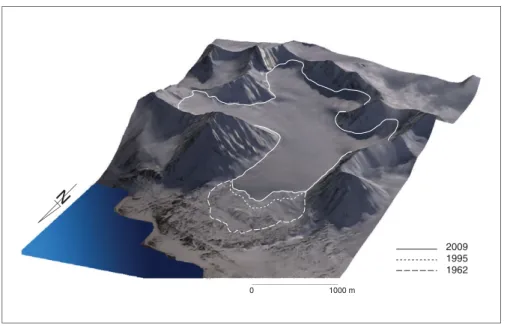
Our study area focuses on the Austre Lovénbreen in the Brøgger peninsula, Spitsbergen, Norway (79◦N). The glacier itself extends from an altitude of 100 m to 550 m above sea level (Fig. 1). This site was selected, amongst the various surrounding glaciers already under investigation, for its specific hydrological configuration in which all runoff water is concentrated in two channels thanks to the geological configuration of the basin. Being
near to the former mining town of Ny-Ålesund, this site has been the focus of intense scrutiny since the 1960s. Amongst the historical dataset collected, the following elevation models are considered:
1. 1/25000 map traced by German scientists between 1962 and 1965 in the framework of the ‘Deutschen Spitzbergen-Expeditionen 1962–1965 des Nationalkomitees für Geodäsie und Geophysik der DDR’ (Pillewizer 1962). Contour lines were digitized and a DEM was generated using non-linear TIN interpolation method. This dataset will be referred to as the ‘1962 map’ since the Austre Lovénbreen snout was mapped at this date,
2. A 1995 DEM from the Norsk Polarinstitutt was derived from six stereo-overlapping aerial photographs taken in August 1995 (Rippin and others 2003; Kohler and others 2007),
3. Airborne LiDAR data collected in 2005 by a team of the Scott Polar Research Institute, Cambridge (Arnold and others 2006; Rees and others 2007) working on the Midtre Lovénbreen and partly covering Austre Lovénbreen. The resulting DEM will be used as reference in assessing the DEM data quality (0.15m vertical accuracy).
4. 2007 SPIRIT (CNES) dataset (Korona and oth-ers 2009) was obtained from stereography of couples of September 2007 SPOT satellite HRS images (high stereoscopic resolution), including the cross-correlation magnitude maps as assess-ment of the quality of the processing for each pixel,
5. Skidoo tracked dual-frequency GPS in 2007 and 2010 over the glacier surface only, with RINEX post-processing and snow thickness removal in the latter case. Removing the snow thickness from a DEM acquired a given spring yields DEM for the end of the summer of the previous year. In this specific case, the processed April 2010 GPS dataset will be considered as the 2009 reference for the computation of ablation rates and mass balances.
All datasets were re-sampled to a 5mx5m pixel size using a nearest neighbour method in order to obtain DEMs at a common spatial resolution.
Altitude resolution estimate
Although our interest is towards the estimate of the glacier mass balance, all the discussion will be about altitude and altitude variations. A conversion to mass balance requires additional in situ measurement of the snow and ice density which will not be discussed in this paper.
A few manually selected points over areas the elev-ations of which are known to have been hardly affected over time are used as reference in a preliminary dataset
N
0 1000 m
2009 1995 1962
Fig. 1. 3D view of the Austre Lovénbreen DEM mapped with a satellite image. The dashed line is the 1962 glacier front limit, the dotted line is the 1995 glacier front limit, and the solid line is the current (2009) glacier front limit, at an altitude 100 m above sea level.
quality assessment of the historical datasets, as shown in Table 1. This processing uses 100 points regularly distributed on a 90 m× 90 m grid located in a rocky re-gion assumed not to evolve over the timescale of this analysis. The typical standard deviation between multiple datasets is in the 1 m to 4 m range, depending on the region under consideration. Such results are consistent with similar analysis performed on the rocky slopes and passes surrounding the glacier basin, even though slopes exhibit the worst results. On the other hand, assessment of the 2010 GPS dataset in the moraine is performed by analysing the tracks followed when driving to the glacier:
40 points along the track, where little snow accumulates, exhibit a standard deviation of 0.6 m when subtracted with all other DEMs, and an average bias of−3.3 m with respect to the 1995 NPI DEM,−1.2 m with respect to the 2005 LiDAR and 0.8 m with respect to the 2007 SPIRIT DEM.
This preliminary dataset, based on a map and DEMs extracted from photogrammetric methods, indeed seems to confirm that small ablation rate will only be detect-able after long time intervals, typically 10 to 12 years (Haakensen 1986). Furthermore, removing a constant off-set is inefficient in solving the issue, since the discrepancy Table 1. Elevation of a few selected points in historical DEMs known not to evolve over time: the observed discrepancies are attributed either to DEM interpolation artifacts or measurement uncertainty. Each analysis is performed on a 90mx90m grid, using points 10m apart (total of 100points), centred on the coordinates provided in the second line, in the Little Ice Age moraine and in a sandur area assumed not to move over time. For each area under consideration, the mean elevation difference (m, in m) and standard deviation (s, in m) is computed. The Fig. illustrates the location of the selected reference areas.
DEMs location 1 location 2 location 3
UTM coordinates 437829, 8759323 438115, 8760266 439424, 8759973 map 1962-NPI1995 m= 4.1, s = 1.0 m = 1.9, s = 4.6 m = 2.3, s = 3.4 map 1962-LiDAR 2005 m= 3.6, s = 4.5 m = 0.6, s = 1.0 m = 2.7, s = 3.6 map 1962-SPIRIT 2007 m= 0.6, s = 5.7 m = 7.4, s = 1.1 m = 4.7, s = 2.5 NPI 1995-LiDAR 2005 m= 0.7, s = 0.3 m = 1.7, s = 1.0 m = 0.4, s = 1.0 NPI 1995-SPIRIT 2007 m= 3.3, s = 1.2 m = −1.3, s = 6.7 m = 2.4, s = 4.7 LiDAR 2005-SPIRIT 2007 m= −3.0, s = 6.5 m = 2.6, s = 1.2 m = 2.0, s = 4.7
THE RELEVANCE OF DIGITAL ELEVATION MODELS TO EVALUATE GLACIER MASS BALANCE 5 elevation (m) elevation (m) elevation diff. (m) elevation diff. (m) pixel position (5 m/pixel)
pixel position (5 m/pixel)
GPS2007 200 400 600 800 200 400 600 800 1000 1200 0 200 400 600 800
pixel position (5 m/pixel)
pixel position (5 m/pixel)
SPIRIT2007 200 400 600 800 200 400 600 800 1000 1200 100 200 300 400 500 600 700
pixel position (5 m/pixel)
pixel position (5 m/pixel)
zoom SPIRIT−GPS 50 100 150 50 100 150 200 SPIRIT−GPS
pixel position (5 m/pixel)
pixel position (5 m/pixel)
200 400 600 800 200 400 600 800 1000 1200 −200 −100 0 100 200 300 −15 −10 −5 0 5
Fig. 2. Two datasets – SPIRIT DEM obtained from stereographic satellite images, and a skidoo-tracked dual-frequency GPS receiver – are acquired during the same year, and are compared to estimate the error (bias and standard deviation) due to DEM processing. The obvious dis-crepancies visible on the southern and western parts of the glacier, yielding elevation errors up to 300m and −200m, are indicated as unreliable pixels by the mask file provided in ad-dition to the SPIRIT dataset and should not be considered, as shown in the bottom right zoom.
from one dataset to another is distributed both in the positive and negative error sides.
The remaining issue concerns the use of newer tech-nologies for establishing DEMs. While a 10 to 20 year in-terval is sufficient for analysing historical datasets separ-ated by such durations, the 4 year continuing programme requires better time resolution while still requiring the spatial resolution provided by DEM analysis. Amongst the latest technologies available, in complement to satel-lite and aerial imagery are airborne LiDAR and dual frequency GPS receivers. Both latter strategies claim sub-decimetre altitude resolution, and are thus appropriate for establishing mass balances between time intervals measured in years rather than decades.
Two datasets acquired under similar conditions in 2007 are obtained by processing skidoo-tracked GPS receiver altitude measurements on the one hand, and the SPIRIT DEM obtained by photogrammetric processing of stereoscopic SPOT satellite images on the other. Sub-tracting these two datasets allows for an assessment of the error observed on each DEM, without being able to attribute all discrepancies to a single method.
Pho-togrammetric processing on feature less arctic areas is prone to cross-correlation attribution error when pro-cessing the stereographic dataset, while GPS is known to exhibit up to several metre uncertainty in altitude measurement, especially in high latitude regions where GPS coverage is poorer due to the GPS satellite con-stellation orbiting at 55◦ inclination (Fig. 2). Subtract-ing the two datasets interpolated on a 5mx5m pixel grid, the altitude difference standard deviation on the flattest region of the glacier (close to its thickest ice position) is 3.0 m, but most worrying is the average difference value of −5.8m. This trend is consistent with the results observed for historical DEMs obtained from maps and processing of aerial stereographic images (Table 1).
Two datasets allow for the assessment of such ideas: a DEM generated from airborne LiDAR measurement was provided by Rees and others (Arnold and others 2006) with a partial coverage of the glacier in which we are interested, and a DEM of the glacier elevation was mapped using a Trimble Geo-XH dual-frequency receiver, followed by an electromagnetic delay correction
elevation (m) elevation (m) elevation diff. (m) elevation diff. (m) LiDAR 05 100 200 300 100 200 300 400 500 0 100 200 300 400 500 600 700 GPS 10 100 200 300 100 200 300 400 500 0 100 200 300 400 500 600 700 300:350,123:170 10 20 30 40 10 20 30 40 50 −5 −4.5 −4 −3.5 −3 −2.5 LiDAR−GPS 100 200 300 100 200 300 400 500 −20 0 20 40
Fig. 3. Comparison of the 2010 GPS field measurements and 2005-LiDAR data provided by Rees (Arnold and others 2006), partially covering the glacier in which we are interested. The selected region, known to be flat and subject to little ablation thanks to its distance to the glacier snout, exhibits a standard deviation in the sub-m range salt= 0.60m, the general trend observed between the two datasets (mean
value of the altitude difference:−4m) being attributed to the ice thickness evolution between the 5 years time lapse. Although the skidoo tracks are still visible on the bottom right figure with the selected interpolation, the resulting error bar is not affected by the various interpolation schemes.
during post-processing of the acquired data using the reference RINEX correction files provided by the local (<10 km away) Ny-Ålesund geodetic station (Fig. 3).
An analysis of the RINEX-corrected dual-frequency GPS data gathered during April 2010 is provided in Fig. 4. For each intersection of the tracks gathered during a 2 week duration, two points at most 5 m apart are located. The histogram of the altitude difference between these points is plotted in Fig. 4 (right). 68% of all altitude differences lie within the± 0.5 m range, with an average value of 0. Such a result is consistent with the classically accepted standard deviation value on the altitude of kinetic tracks post-processed using RINEX data on a km long baseline (Xu 2007; GAMIT 2000). Assuming the most precise data being provided by LiDAR, the difference between the 2005 LiDAR altitude map and 2010 skidoo-tracked dual-frequency GPS altitude map exhibits a standard deviation of 0.60 m and an average value of −4 m in the flattest (and thickest) part of the glacier (Fig. 3), without snow thickness subtraction since
this calculation is performed on the raw data. Although the average value difference is significant, the data quality improvement is clearly stated by the reduction in the altitude scale from 25 m at full scale (Fig. 2 bottom right) to 3 m (Fig. 3 bottom right).
Hence, the GPS dataset altitude uncertainty is of the same order of magnitude than the standard deviation ob-served for airborne LiDAR measurements, and displays the limit below which experimental errors of surface elevation measurements become significant over ranging errors.
Results and discussion
Having assessed the altitude resolution of each data-set, we now focus on the estimate of the mass-balance calculation by subtracting DEMs and estimat-ing the shortest time interval for which mass balance evolution is reliably computed above the altitude-uncertainty.
THE RELEVANCE OF DIGITAL ELEVATION MODELS TO EVALUATE GLACIER MASS BALANCE 7 12.08 12.1 12.12 12.14 12.16 12.18 12.2 12.22 12.24 12.26 78.85 78.86 78.87 78.88 78.89 78.9 78.91 78.92 longitude WGS84 (deg) latit u de WGS 8 4 (deg) 0 2 4 6 8 10 12 14 -2 -1.5 -1 -0.5 0 0.5 1 1.5 2 pro b a b ility (\%) altitude difference (m) (1:2000) ; (6500:10000) ; (15000:end)
Fig. 4. Map of the skidoo tracks (lines) followed while mapping the glacier elevation, while sampling the GPS position at 1Hz rate: each dark circle indicates the intersection of two tracks with measurement points separated by a distance of less than 5 m in the latitude/longitude plane. The histogram (right) summarises the altitude difference between each one of these point pairs.
In situ annual ablation stake measurements will be used to assess the time interval beyond which the alti-tude standard deviation becomes larger than the yearly accumulation or ablation level (Fig. 5). Assuming that the average value of the altitude difference between the SPIRIT DEM and 2007 GPS measurements is due to an offset attributed to the stereographic image processing, subtracting the two GPS datasets acquired in 2007
frequency, including snow cover) and 2010 (dual-frequency and RINEX post-processing, including snow cover) yields a total volume loss between 8.0 and 6.7 M m3depending on how the measurements over the gla-cier area are stitched to the surrounding mountain eleva-tion model (the lower bound resulting from the removal of obvious interpolation errors close to the steepest slopes around the glacier basin, Fig. 6). Since the glacier area is
Accumulation / ablation (in cm) + 343 - 596 0 - 300 - 100 + 30 + 90 + 189 - 218 0 Accumulation / ablation (in cm) - 28 cm - 37 cm - 37 cm - 102 cm 2007 - 2008 2008 - 2009 2009 - 2010 2007 - 2010 4.590 km2 glacier surface 2.382 km2 accumulation 2.208 km2 ablation a b ELA
ELA ELA ELA
Fig. 5. Glacier mass balance measured for the years 2007–2008, 2008–2009, and 2009–2010, using ablation stakes, and interpolated over the glacier basin area. The 2007–2010 mass balance calculation from the interpolated ablation stake measurements is computed for comparison with the GPS dataset subtraction (Fig. 6).
Fig. 6. Volume loss of the glacier between 2007 and 2010 based on the subtraction of DEMs acquired using skidoo-tracked GPS receivers. Some of the most obvious errors, associated with the difficulty of connecting the GPS-based DEM with the surrounding mountain DEM (extracted from aerial photography cross-correlation), yield a significant un-certainty (15%) as illustrated by the comparison between the raw subtracted data (volume difference of 8.0 M m3),
and after removal of the most obvious discrepancies close to the steepest slopes (volume difference of 6.7 M m3): all
subtracted values below –10 m were set to 0, as shown in the white areas. 1962–1995 1995–2009 1962–2009
measured to be 4.8km2, the average ablation is in the 1.7
to 1.4m range on average, with the most visible altitude losses in the glacier snout at a rate of−5 to −7m over the 3 year period (consistent with the above mentioned aver-age ablation rate).
When subtracting the 1962 map based DEM and the 2010 GPS based DEM, the glacier snout ablation rate is 70m over the 47year duration (the processed 2010 GPS dataset is representative of the 2009 summer glacier state), or an average 1.5m/year, consistent with the latest stake measurements (Fig. 5). This ablation rate at the glacier snout is in accordance with results provided in the literature for other glacier basins in the same area (Barrand and others 2010). A quantitative comparison of the estimated mass balance from ablation stakes and DEM is performed by comparing the interpolated field stake measurements provided in Fig. 5 and the DEM difference exhibited in Fig. 6.
Mapping the ablation and accumulation spatial dis-tribution extends the concept of equilibrium line altitude (ELA) to a spatially resolved concept for a polar gla-cier with little altitude variation, where an equilibrium line is mostly defined by local climate conditions (wind orientation, slope orientation with respect to the sun position) rather than by altitude as is familiar for valley glaciers. Fig. 7 exhibits the spatial distribution of accu-mulation areas as a function of space and time interval, clearly located in the cirques at highest altitudes. No area of accumulation is observed during the 1995–2009 period.
The result of this analysis is consistent with the trend reported for most glaciers in the Brøgger penin-sula: strong ablation on most of the glacier, increased in the last years with which this study is most con-cerned. The observed ablation rate is averaged over the whole glacier area to reach 0.43m/a during the 1962– 1995 period, increasing to 0.70m/a for the 1995–2009 period. These results, obtained from DEM subtraction, are significantly larger than those obtained from in situ ablation stake measurements, with average ablation rates of 0.28, 0.37 and 0.37m/a for the 2007–2008, 2008–2009 and 2009–2010 periods respectively. Both the yearly ablation rate and overestimate of the DEM calculation with respect to ablation stakes are consistent with previ-ous analysis of measurements performed on the nearby Midtre Lovénbreen (Rees and others 2007) – 0.70m/a (DEM difference) for the 2003–2005 period and 0.4m/a (ablation stake) for the 1977–1995 period respectively. Indeed, DEM subtraction appears to overestimate the ablation rate with respect to in situ stake measurements (Francou and others 2007; Pope and others 2007).
Considering the elevation accuracy needed to assess the ablation rate on time scales of only a few years, snow cover might be significant, yielding a bias on the height measurements: 0.3 to 3.0 m snow thicknesses have been observed from the snout to the cirques respectively, with average thicknesses ranging in the 1.5 to 2.0 m range between 2008 and 2010, as observed by snow drills (interpolated data, data not shown). While snow cover might be negligible at the time when airborne LiDAR
THE RELEVANCE OF DIGITAL ELEVATION MODELS TO EVALUATE GLACIER MASS BALANCE 9
Fig. 7. Map of the pixels exhibiting accumulation (light colour areas) and ablation (dark colour areas): the DEM method provides a high resolution spatial information, exhibiting strong ablation at the glacier snout mostly visible on the field as a glacier snout retreat.
measurements are performed (end of the summer, in the July-August), it induces a significant bias on skidoo-tracked GPS measurements which can only be performed when the snow thickness is highest, in April-May. Re-moving the interpolated snow thickness measured by in situ snow drills, in our case 47 measurement points over the glacier, yields an ice elevation from the previous year. This time difference becomes significant when calculat-ing the time interval between two DEM subtractions: DEMs recorded during summer (most remote sensing methods) yield elevation models for the given summer, while in situ recording using GPS (done in April as required by snow cover to drive the snowmobiles) cor-rected for snow thickness provide an elevation model for the summer of the previous year. Such a statement is acknowledged more roughly by Kohler and others when subtracting a constant snow thickness from elevation models due to the lack of detailed in situ measurements (Kohler and others 2007). DEM derived ablation rates and the fact that ablation is apparently occurring all over the glacier are unexpected results. Although these results are consistent with the literature (Kohler and others 2007; Pope and others 2007; Rippin and others 2003), some aspects require a cautious assessment. Indeed, all refer-ences observe no significant area of accumulation in the latest years. A general overestimate of the ablation rate with respect to the ablation stake measurement results from DEM subtraction, as stated by Pope and others (2007). Such a statement is to be compared with continu-ous digital picture acquisition (Laffly and others 2011) and in situ ablation stake measurements. Images exhibit continuous snow cover in the cirques, even during the whole summer season, in disagreement with the albedo change hypothesis stating that during the snow melt,
bare ice is exposed yielding albedo decrease (Kohler and others 2007). During the last 3 years, ablation stake length had to be increased every year in the upper part of the glacier, which confirms accumulation. On the other hand, DEM subtraction ablation rate is above the error bar and hence significant. This is especially true for the latest period under consideration (1995–2009), during which the standard deviation over elevation measurements is below 1.2 m. These opposite conclusions are striking and deserve further analysis to be fully understood, each method measuring different properties. This variability in observed changes should lead to a careful use of DEM difference in mass balance computation. While ablation stakes account for relative surface accumulation, a DEM records absolute ice surface altitudes. These measure-ments, different in nature, might reveal phenomena oc-curring at different depths and scale. Further monitoring including ground penetrating radar map time series and ablation stake tip monitoring, for example using a ground based LiDAR, from fixed points over rocky areas might reveal such different processes.
Conclusion
Having reminded the reader of some of the drawbacks of historical DEM generation methods from remote sensing sources (aerial and satellite images) in polar regions due to the lack of reference point to map the cross-correlation distance, we demonstrate the use of more recent tech-nology, namely RINEX-corrected dual-frequency GPS receiver and a comparison with airborne LiDAR datasets acquired by other authors, as means to improve by at least one order of magnitude the altitude resolution of DEMs. With such precise datasets, glacier mass balances
within time intervals of a few years can significantly be estimated by subtracting successive DEMs.
Technology providing the means to measure an alti-tude with sub-m resolution, the remaining sources of errors are associated with the experimental protocol (time of the year when the measurements are performed, remaining snow thickness and quality when perform-ing skidoo-tracked GPS elevation mappperform-ing) and data processing (subtracting the snow thickness in order to compute mass balance based on the altitude of firn). The time interval beyond which DEM difference provides a significant estimate of the mass balance of a polar glacier is estimated to be 3 years, as defined by an ablation at the glacier snout larger than three DEM altitude standard deviations: at an average ablation rate of 0.63m/a, the 0.50m standard deviation is reached every year.
This study has focused on DEMs specifically gen-erated from various sources (maps, aerial stereographic photography, skidoo-tracked GPS). However, beyond the acquisition of research programme related datasets, sev-eral global DEM mapping projects are under investig-ation, which might provide additional information with improved time resolution. Since most automated signal processing procedures on image datasets are inefficient in the low contrast polar regions, dedicated processing of existing datasets, including the ASTER satellite dataset automatically processed to generate the GDEM, might provide some missing data in time intervals that were not otherwise covered. Furthermore, multiple high resolution space-borne RADAR mapping programmes, insensitive to cloud cover and providing surface property inform-ation complementary to surface elevinform-ation (snow or ice coverage), will provide the necessary data to improve the use of DEM in estimating glacier mass balance evolution in the coming years. The issue of how DEM measurements relate to ablation stake in situ measure-ment should however be answered if such tools are to be used as glacier evolution indicators: a comparison of ground based ablation stake tip altitude monitoring from a fixed reference point and simultaneous classical stake characterisation might provide invaluable insight into such topics.
Acknowledgements
Funding for this research programme was provided by the French National Research Agency (ANR) Hydro-Sensors-FlOWS program, IPY #16 programme, and IPEV. W.G. Rees (Scott Polar Research Institute) provided the LiDAR dataset acquired during a Midtre Lovénbreen mapping campaign. J. Kohler and H.F. Aas (Norsk Polarinstitutt) provided the part of a 1995 DEM over the Austre Lovénbreen. CNES (Centre National d’Étude Spatial) funded the SPIRIT dataset (in the frame of the IPY), resulting from the processing by IGN (Institut Géographique National) of SPOT (Satellite Pour l’Observation de la Terre) stereoscopic images. É.
Berthier is acknowledged for providing support during the analysis of this dataset.
References
Arnold, N.S., W.G. Rees, B.J. Devereaux, and G. Amable. 2006. Evaluating the potential of high-resolution airborne LiDAR in glaciology.International Journal of Remote Sensing27 (5– 6): 1233–1251.
Barrand, N.E., T.D. James and T. Murray. 2010. Spatio-temporal variability in elevation changes of two high-Arctic valley glaciers.Journal of Glaciology56(199): 771–780.
Escher-Vetter, H. 2000. Modelling meltwater production with a distributed energy balance method and runoff using a linear reservoir approach – results from Vernagtferner, Oetzal alps, for the ablation seasons 1992 to 1995. Zeithschift für Gletscherkunde und Glazialgeologie 36: S119– 150.
Francou, B., and C. Vincent. 2007.Les glaciers à l’épreuve du climat. Paris : IRD Edition.
GAMIT. 2000. Documentation of the GAMIT GPS Ana-lysis Software 2. URL: http://chandler.mit.edu/∼simon/gtgk/ GAMIT.pdf.
Haakensen, N. 1986. Glacier mapping to confirm results from mass-balance measurements.Annals of Glaciology8: 73– 75.
Hansen, S. 1999. A photogrammetrical, climate-statistical and geomorphological approach to the post Little Ice Age changes of the midre Lovén-breen glacier, Svalbard. Unpublished M.Sc. dissertation. Copenhagen: University of Copenhagen.
Kohler, J., T.D. James, T. Murray, C. Nuth, O. Brandt, N.E. Barrand, H.F. Aas, and A. Luckman. 2007. Acceleration in thinning rate on western Svalbard glaciers.Geophysical Research Letters34: L18502.
Korona, J., É. Berthier, M. Bernard, F. Rémy, and É. Thouvenot. 2009. SPIRIT. SPOT 5 stereoscopic survey of polar Ice: refer-ence images and topographies during the fourth International Polar Year (2007–2009).ISPRS Journal of Photogrammetry and Remote Sensing64: 204–212.
Laffly, D., É. Bernard, J.-M Friedt, G. Martin, F. Tolle, C. Marlin, and M. Griselin. 2012. High temporal resolution monitoring of snow cover using oblique view ground-based pictures.Polar Recordin press.
Østrem, G., and M. Brugman. 1991. Glacier mass balance measurement–a manual for field and office work. Oslo: The Norwegian water resources and energy administration. Paterson, W.S.B. 2000.Physics of glaciers3rd edition, Oxford:
Butterworth-Heinemann.
Pillewizer, W. 1962. Deutsche Spitzbergenexpedition 1962. Petermanns Geographische. Mitteilungen 106(4): 286. (Translation in English available at URL: http://handle. dtic.mil/100.2/AD406986).
Pope, A., T. Murray, and A. Luckman. 2007. DEM quality assess-ment for quantification of glacier surface change.Annals of Glaciology46: 189–194.
Rees, W.G., and N.S. Arnold. 2007. Mass balance and dynamics of a valley glacier measured by high-resolution LiDAR.Polar Record43: 311–319.
Rippin, D., I. Willis, N. Arnold, A. Hodson, J. Moore, J. Kohler, and H. Björnsson. 2003. Changes in geometry and subgla-cial drainage of Midre Lovénbreen, Svalbard, determined from digital elevation models.Earth Surface. Processes and. Landforms28: 273–298.
Xu, G. 2007. GPS – theory, algorithms and applications 2nd edition. Berlin/Heidelberg: Springer-Verlag.