The Effect of Forecasting Accuracy
on the Sizing of Energy Storage
The MIT Faculty has made this article openly available.
Please share
how this access benefits you. Your story matters.
Citation
Jaworsky, Christina, Konstantin Turitsyn, and Scott Backhaus. “The
Effect of Forecasting Accuracy on the Sizing of Energy Storage.”
ASME 2014 Dynamic Systems and Control Conference DSCC2014,
22-24 October, 2014, San Antonio, Texas, USA, ASME, 2014. © 2014
by ASME
As Published
http://dx.doi.org/10.1115/DSCC2014-6113
Publisher
American Society of Mechanical Engineers (ASME)
Version
Final published version
Citable link
http://hdl.handle.net/1721.1/109305
Terms of Use
Article is made available in accordance with the publisher's
policy and may be subject to US copyright law. Please refer to the
publisher's site for terms of use.
THE EFFECT OF FORECASTING ACCURACY ON THE SIZING OF ENERGY
STORAGE
Christina Jaworsky⇤
Department of Mechanical Engineering Massachusetts Institute of Technology
Cambridge, Massachusetts 02139 Email: jaworsky@mit.edu
Konstantin Turitsyn
Department of Mechanical Engineering Massachusetts Institute of Technology
Cambridge, Massachusetts 02139 Email: turitsyn@mit.edu
Scott Backhaus Center for Nonlinear Studies Los Alamos National Laboratory Los Alamos, New Mexico 87545
ABSTRACT
The purpose of this research is to the problem of optimal sizing of energy storage required for compensation of wind farm generation variability. Using wind farm production data from the BPA, we assess the effect of forecast quality and economic dispatch timing on the size of storage and critical power rat-ing required to nearly perfectly match the committed energy. We develop a Model-Predictive-Control (MPC) based operational model following NERC standard recommendations. Different forecasts are considered and compared from the storage sizing perspective. The results of our simulations can be fit by two sim-ple relations, connecting the storage sizing with forecast error, wind variability, and the timescales of scheduling. A more ac-curate forecast reduces the storage sizing. However, diminishing returns are observed when the forecast error becomes compara-ble to natural wind variability within the commitment time inter-val. The proposed methodology can be extended to other systems with intermittent generation and controllable real or virtual stor-age.
NOMENCLATURE
tC Length of commitment interval
tLA Look ahead time for advance scheduling tD Delivery time interval
Th Forecast horizon Pset Scheduled power
Pdel Delivered power Pl Lost/curtailed power
Pc Power used to charge storage Pd Power discharged from storage Pw Power available from wind h Single trip efficiency of storage Pcap Power capacity of storage Ecap Energy capacity of storage serr Average forecast error
swind Wind power standard deviation during commitment in-tervals
stot Total error
PRMS RMS of the mismatch between delivered and scheduled power
The spacing between abstract and the text heading is two line spaces. The primary text heading is boldface in all capitals, flushed left with the left margin. The spacing between the text and the heading is also two line spaces.
INTRODUCTION
Renewable generation offers a clean and sustainable alter-native to fossil fuel generation. The level of penetration of re-newable resources, especially wind, is expected to reach the fig-ure of 20% in the coming two decades [1, 2]. This transition poses a tremendous challenge to modern power systems that rely on fully dispatchable generation resources. Future power sys-Proceedings of the ASME 2014 Dynamic Systems and Control Conference
DSCC2014 October 22-24, 2014, San Antonio, TX, USA
tems will have to operate in the presence of forecast uncertainty and therefore significant amounts of backup generation or large amounts of electric storage would be required for short term and midterm balancing needs. Rapid advancements in electric-ity storage technologies make them especially attractive for wind integration [3–5]. One particular question that must be answered in any feasibility assessment is the optimal sizing of storage nec-essary to alleviate the intermittency problems of utilizing renew-able resources. This is an unexpectedly difficult question as the answer depends on many parameters. These include, but are not limited to, the technological properties of storage equipment, the statistical characteristics of a renewable generator’s production, and the quality of the forecast available to system operators. In this paper we attempt to address some of these questions, fo-cusing mostly on the least understood question of the value of forecast quality.
Analysis and synthesis of optimal operation schemes is not possible without inputs from atmospheric sciences, statistical forecasting, power systems operation and regulation, and elec-tric storage engineering. One of the first optimal energy stor-age dispatch algorithms for short term markets with heavy wind generation penetration was introduced in [6]. Stochastic secu-rity framework for operational planning was proposed in [7], al-lowing for better efficiency in comparison to more conservative, worst-case scenario approaches. A more sophisticated method of energy storage, where the probability distribution of storage re-quirements was found for a set of scenario forecasts, accounts for the uncertainty of the wind was presented in [8]. It was shown that storage can effectively operate as a separate market entity by hedging against wind power forecast errors and by dynamically sizing storage to increase the efficiency of the system without af-fecting the producer’s profit. Another study, looking at the time to saturation of a storage device’s state of charge given different forecasts, [9] has shown that although large amounts of storage are required to completely compensate for the wind forecast er-rors, an allowance for small amounts of unserved energy dramat-ically reduces the storage size requirements.
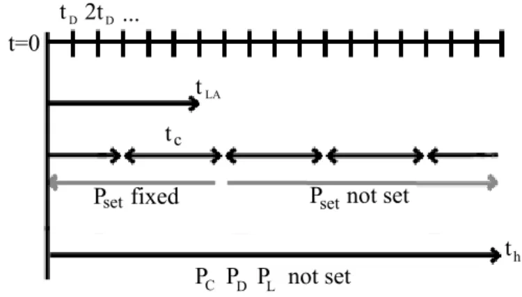
In this paper, analyze the effect of forecast quality on the storage capacity necessary to suppress the variability of inter-mittent wind generation. We consider a mid-timescale service where the energy storage is used to enable a wind farm or an aggregation of farms to maintain a scheduled hourly output af-ter economic dispatch. We use a model that mimics the INT-006-3 request for interchange standard proposed by NERC [10]. Within these guidelines, energy from large generators is typi-cally scheduled in hourly blocks where generators are expected to maintain a relatively uniform power output. To allow time for data collection, optimal scheduling, and generator ramping from one hourly setpoint to the next, generator output for an hour is typically scheduled 90 minutes before its start. The timeline for this process is shown in Fig. 1 and explained in detail in section . This timeline dictates that for energy storage operation
coor-FIGURE 1. TIMELINE OF THE SEQUENCE AND TIME LAGS
BETWEEN THE SCHEDULING THE INTERCHANGE USED IN OUR MODEL OF A GENERATOR CONNECTED TO THE BULK POWER SYSTEM.
dinated with wind generation, the crucial period for forecasting is 90-150 minutes into the future. However, the time-integral constraint imposed by the finite energy storage capacity, Ecap, implies that forecasting is also important at shorter and longer timescales, i.e. it may be beneficial to save capacity for variabil-ity forecasted in the more distant future.
The time-integral constraint and the incorporation of fore-casting are addressed by model predictive control (MPC) of en-ergy storage. Using a convex optimization package, we control the storage device in a way that minimizes the deviation of set power from delivered power over the forecast horizon at each time step. This means an optimization is performed at each time step, however the control method finds the best possible set of actions given the forecast. We incorporate large historical wind generation datasets [11] into extensive simulations of the MPC of energy storage, finding how the residual deviations from the scheduled interchange scale with the storage capacity Ecap, the maximum charge/discharge rates Pcap, and the standard deviation of the forecast errorsserr. The results can be interpreted as rules for using the statistics of historical wind generation and errors in forecasting to appropriately size Ecapand Pcapof a jointly oper-ated energy storage and generation system. By using the hybrid data-driven Monte-Carlo based simulations as an experimental tool, we assess the dependence of the necessary storage capacity and power rating on other system parameters like forecast error and commitment/look-ahead time.
The structure of this paper is as follows: In Model, we de-scribe the market, storage, and MPC control and forecast models used in our study. The results of our simulations and their in-terpretation are presented in Simulation. Analysis and our final predictions are described in Analysis, and our conclusions and future plans are included in the last section, Conclusion.
Model
Market Structure
Wind generators will have to participate in the electricity market to be economically viable. This means that wind gen-eration must be scheduled ahead of time, and a constant power output must be maintained over a production interval. Although wind is intermittent and uncontrollable, with some amount of storage, it is possible to compensate for errors between the ac-tual wind generation and committed power output.
Economic dispatch of electricity generation requires plan-ning traditional fossil fuel and nuclear generators to start up, shutdown, and ramp between set points. Generators must make bids to be scheduled ahead of when they are committed to oper-ate. In our model, we account for scheduling of future generation by introducing a look ahead time, tLA. At all times up to tLA, the generator’s power output has already been scheduled in previous economic dispatch. The generator is scheduled to have constant output, Pset, on commitment intervals of length tC. The produc-tion during these intervals is scheduled when the start of the in-terval is tLAahead of the current time. The set power of future tC intervals can always be changed until their start time reaches tLA, at which point it is scheduled. Power is delivered within each commitment interval on a shorter time scale , called the deliv-ery time, tD. A generator is penalized on each delivery interval for the deviation from the actual delivered power, Pdel, from the scheduled power, Pset. This means that for an intermittent re-source like wind to be a competitor in the electricity market, it must either not use all available generation and curtail wind or incorporate some kind of storage or fast ramping gas generator to correct for imperfect scheduling and wind variability during delivery intervals.
In our simulations, we tested look ahead times of tLA= 30,60 and 90 minutes. Commitment times were set to tC = 15,30,45 and 60 minutes. Deliveries were always made on 15 minute intervals of tD=15 minutes . The time horizon, Th, on which a forecast of future generation was available, was set to 270 minutes from the current time. Other time horizons were considered but did not affect the results.
Wind Generation and Storage
We consider a simple model of a wind farm and ESS. Our model captures the main statistical characteristics of the wind and technological constraints associated with the storage. We aggregate all wind generation into a single source, and we ag-gregate all ESS as a single storage device connected to the grid. ESS can either be located on the site of the wind generation or connected elsewhere. However, because we do not model trans-mission losses or congestion, our model only applies to cases where transmission to the storage devices is not constrained by the grid. We allow exchange of power between the renewable generator, storage device, and external grid. The details of the
interconnections are not modeled. We assume that the energy captured from the wind can be transferred either directly to the external grid or routed to the storage system and transferred to the grid at later times. To describe power flow and energy state in the storage device, we use the following set of equations with discrete time steps of tD:
Pdel(t) = Pw(t) +hPd(t) Pc(t) Pl(t) (1)
E(t +DT) = E(t) + hPc(t)DT Pd(t)DT (2) where, Pdel(t) represents the average power delivered to the grid during the time intervalDT, and Pw(t) is the power delivered from the wind farm. The process of storage charging is repre-sented by the average charging and discharging rates, Pc(t) and Pd(t). The single trip efficiency is represented by coefficienth, set to .8 for this study. We ignore the self-discharge rate, assum-ing that the energy lost to self-discharge is small relative to the total amount of energy flowing through our system. Finally, we account for the effect of wind curtailment in the system with the variable Pl(t). Curtailment can happen either at the wind turbine control level or at the point of interconnection of our aggregate system with the external grid.
We used the BPA wind generation time series [11] to sim-ulate one week of wind generation. The capacity of the wind generation in the BPA system increased over time, so separate simulations were performed for the years 2007-2011. Within this timeframe, the total installed wind capacity increased from 700 to 3500 MW. The weeks used in the simulations were chosen from different months to prevent any kind of seasonal bias. Optimization and MPC of storage
Our model uses MPC to optimize the storage control, wind curtailment, and generation scheduling. The MPC is run on every time step and looks ahead over Th. On the interval t02 [t,t + Th], all the values Pd(t0),Pc(t0)and Pl(t0)are available for optimiza-tion. However, only Pset(t0)for commitment intervals that start after the look-ahead time, t0>t + tLA can be controlled. This means the MPC uses storage and curtailment to adhere to the pre-viously set schedule to the best of its ability and chooses a future Psetschedule based on the forecast. Typically, the MPC chooses future Pset to be close to the mean of predicted wind generation during the corresponding commitment time interval. For each time step, the MPC attempts to minimize the squared deviation of the mismatch between the committed and actually delivered power, (Pdel Pset)2, for each delivery time interval seen in the control horizon.
In our model, storage technology and the interconnection properties are incorporated via constraints. The constraint Ecap restricts the total amount of energy that can be stored in the stor-age system at any moment of time: 0 E(t) Ecap, given by Eqn.(6) . Next, we limit the charge and discharge rate of stor-age. In real systems, this constraint can either represent the power rating of the storage system or the transmission limits of the interconnection system: 0 Pc(t),Pd(t) Pcap, Eqn. (7). We assume that no power can be drawn from the grid, which is accounted for with the inequalities Pdel(t),Pl(t) 0, Eqn. (8). We have also constrained the overall levels of system ef-ficiency,ÂT
t=1(Pl(t) +hPc(t) +hPd(t)) 0.01ÂTt=1Pw(t), Eqn. (9), meaning 99% of the energy available from the wind must eventually be delivered to the grid. The overall system efficiency ensures that the wind turbine system produces power, preventing trivial solutions where huge amounts of power are curtailed.
The above discussion can be summarized in the following optimization problem: min Pc,Pd,Pl,Pset,Pdel Th
Â
t=1 (Pdel(t) Pset(t))2 (3) subjectto : Pdel(t) = Pw(t) +hPd(t) Pc(t) Pl(t), (4) E(t +DT) = E(t) + hPc(t)DT Pd(t)DT, (5) 0 E(t) Ecap, (6) 0 Pc(t),Pd(t) Pcap, (7) Pg(t),Pl(t) 0 (8) TÂ
t=1 (Pl(t) +hPc(t) +hPd(t)) 0.01 TÂ
t=1 Pw(t) (9) The optimization is performed with respect to the values Pc(t0),Pd(t0),Pl(t0)on the interval t02 [t,t + Th]and with respect to the values of Pset(t0)on the interval t02 [t +tLA,t + Th].Forecast Models
In the absence of real forecast data, we use two artificial forecast models in our studies. The forecast of the wind is up-dated at each time step according to one of the following proce-dures:
Forecast A: Gaussian. In the first model of forecast, we add Gaussian noisex(t0)to the wind time series to forecast of future generation, ˜Pw(t0) =Pw(t0) +x(t0), where t02 [t,t +Th]. The values of the noise are statistically independent at every mo-ment of time and their mean value is zero, hx(t0)i = 0. The vari-ance of the noise scales over the forecast horizon to represent more uncertainty in future events. To compare forecasts of dif-ferent qualities, we introduce the standard deviation of the
fore-cast error,serr. We calculateserrby averaging the error over the interval [t +tLA,t +tLA+tC], the time interval where Psetwas cho-sen. The Gaussian forecast models the persistence and changes in wind generation and mimics the high-quality forecasts avail-able from meteorological measurements.
Forecast B: Persistence. The second forecast model simulated is a persistence model. Two variations are considered: one where the wind maintains the same average output as the previous hour and one where it follows a linear fit of the pre-vious hour’s generation. The persistence model is not as real-istic as the Gaussian model because it does not take into con-sideration the availability of meteorological measurements and weather models that forecast wind power production. The persis-tence model causes gross over and underestimation of the avail-able wind power over the forecast horizon. Storage requirements for persistence forecasting are more than an order of magnitude greater than for the Gaussian forecasting. Therefore, a forecast that has information about future wind events permits a smaller and less expensive storage device.
Simulation Results
The performance of our generation and storage model was measured by considering the RMS error of the scheduled and delivered power mismatch:
PRMS= s 1 T T
Â
t=1 [Pdel(t) Pset(t)]2 (10) where, T is one week for each data set. We have primarily fo-cused on assessing how the RMS error depends on the quality of a forecast and the capacity and charging rate of a storage system. Forecast TechniquesPersistence forecasts underperformed. Unless we consid-ered unrealistically large storage capacities, the RMS error was substantial. Simulations showed that the Psetscheduled were dif-ferent from the actual behavior of the wind, and the ESS was unable to compensate for the errors in prediction. The persis-tence forecasts did not use any information about the future wind behavior, and, as a result, the forecast made at tLAminutes in the forecast horizon inaccurately represented the actual wind.
Forecasts with a Gaussian error yielded better results, and all further analysis is derived from this forecast model. Energy capacities equivalent to storing a few minutes of maximum wind farm generation were shown to reduce the RMS error substan-tially, seen in Fig. 2. Forecast A was able to forecast the shape of the future wind profile, correctly predicting the important events and changes in wind generation over the forecast horizon. The
Gaussian forecast was not misrepresenting the behavior of the wind at the moment critical for scheduling, t +tLA. Because there was a accurate representation of the wind behavior, the optimal Pset found was close to what the actual realization of the wind was.
Identifying Critical Values of Parameters
To size storage, we plot the storage property against its RMS performance. We observed a trend of a steep decrease of error followed by constant error, shown in Fig. 2 for storage capacity and Fig. 3 for power rating. This indicated that there was a crit-ical value of storage capacity, Ecap⇤ , and power rating, Pcap⇤ , be-yond which there was no performance increase with larger stor-age properties. At this critical point, the storstor-age system had the minimal values of its properties, where the error is nearly re-moved, therefore Ecap⇤ and Pcap⇤ were the cheapest storage option. While there is no harm in oversizing storage, it adds to the ex-pense of using renewable generation.
Wind Variability versus Energy Capacity
In the first series of experiments, we simulate the operation of storage without any constraints on the power rating, Pcap! •. We set tC=1 hour and tLA= 90 minutes. For each dataset, we find the E⇤
cap(s) required to drive PRMSto its asymptotic value. The value of E⇤
capdepends on the deviations of the wind from the scheduled power, Pset. The deviations occur both from the natural variability of the wind within the commitment interval, swind, and the error in the forecast,serr.
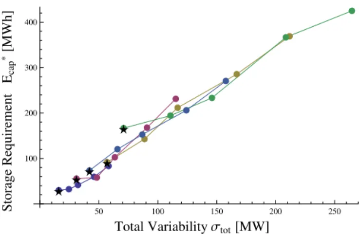
In our simulations of datasets from different years, we ob-serve a wide range of natural wind variability. We scale the fore-cast error with the total capacity of the wind generation. Fig. 4 shows the correlation between the required storage capacity and the total variability in the wind. Ecap⇤ can be approximated by the following expression: E⇤ cap=twind q s2 wind+serr2 , (11)
where,twindwas found to betwind⇡ 1.6 hours for the one hour commitment time interval. With no forecast error, Pset(t) is per-fectly scheduled, and the storage only mitigates the natural vari-ability of the wind generation with commitment intervals, char-acterized by the standard deviation, swind. When forecast er-ror is introduced to the model, storage must also compensate for incorrect predictions of the scheduled power. The inclusion of forecasting error changes the total deviation of the wind to stot= q s2 wind+serr2 . RM S Er ror @MW D 100 200 300 400 10 20 30 40 50 152 MWh 117 MWh 76 MWh 51 MWh Prediction Error Storage Capacity@MWhD
FIGURE 2. POWER FLUCTUATIONS, AS MEASURED BY PRMS,
VERSUS THE ECAP FOR AN UNCONSTRAINED PCAP FOR A
RANGE OF FORECAST ERRORSsERR. CRITICAL STORAGE
CA-PACITY E⇤
CAP IS THE VALUE OF ENERGY CAPACITY WHERE
PRMSREACHES ITS ASYMPTOTIC VALUE.
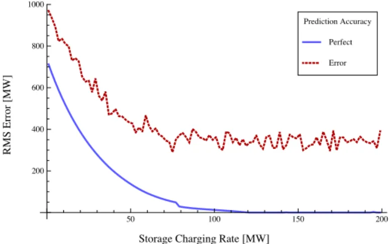
RM S Er ror @MW D 50 100 150 200 200 400 600 800 1000 Error Perfect Prediction Accuracy
Storage Charging Rate@MWD
FIGURE 3. PRMSVERSUS PCAPFOR PERFECT (DASHED) AND
IMPERFECT (SOLID) FORECASTING. EACH PLATEAUS TO A CONSTANT VALUE AT THE SAME POWER RATING. IN THESE SIMULATIONS, THE STORAGE ENERGY CAPACITY WAS SET
AT E⇤
CAP(sERR). NOTE THAT THE SATURATION OF THE
PER-FECT FORECAST PLOT HAPPENS AT EXTREMELY LOW PRMS
VALUES.
Commitment Time versus Energy Capacity
To understand how the storage requirements were affected by the scheduling timescales, we ran simulations with different commitment intervals tCfrom 15 to 60 minutes. For consistency, we kept tLAat 90 minutes and tDat 15 minutes. Longer time com-mitment intervals required more storage for the same amount of
Storage Requirement Ecap ! !MWh "
!
!
!
!
!
50 100 150 200 250 100 200 300 400Total Variability Σtot!MW"
FIGURE 4. THE REQUIRED STORAGE CAPACITY IS
DI-RECTLY PROPORTIONAL TO THE TOTAL AMOUNT DEVIA-TION OF THE WIND. EACH COLOR REPRESENTS A DIFFER-ENT YEAR OF DATA. THE STARRED DATA POINTS SHOW THE CASES WHERE THERE IS A PERFECT FORECAST AND
ONLY NATURAL WIND VARIABILITYsW INDAFFECTS THE
RE-QUIRED STORAGE CAPACITY.
total variability because the scheduled power had to be main-tained at a constant value for a longer time period. We found that the value oftwind, the slope in Eqn. (11), scales linearly with tC. In Fig. 5 we show the dependence of Ecap⇤ onstot and tC. For each tC, a different slope relating how critical storage capacity Ecap⇤ scaled with total errorstot was found. The required stor-age capacity scales linearly with the length of tC. Based on these observations, the following formula is proposed relating the ca-pacity, variability and commitment time:
E⇤
cap=1.6tC q
s2
wind+serr2 , (12) The coefficient 1.6 might be related to the properties of Gaus-sian noise because it is proportional to exactly twice the average expected absolute deviation from the mean for Gaussian noise. Although we don’t have a model supporting this conjecture, it might be worthwhile to check if this observation holds for other statistical forecast error models.
Storage Capacity versus Look Ahead Time
Next, we tested how the look ahead time tLAaffects the criti-cal amount of storage Ecap⇤ required to suppress the power output fluctuations. We tested tLAin the range of 30 to 90 minutes and found that the value of Ecap⇤ did not experience any significant changes. The results of the corresponding simulations are shown on the Fig. 5. The amount of time ahead a schedule is set does
Storage Requirement per Unit Error Ecap ! ! Σtot "h # 0.0 0.2 0.4 0.6 0.8 1.0 0.5 1.0 1.5 2.0 Commitment Length tc"h#
FIGURE 5. THE STORAGE COMMITMENT PER UNIT ERROR
(SLOPE OF FIG. 4 FOR 1 HOUR) SCALED LINEARLY WITH TC.
THE DIFFERENT COLORS SHOW TLA=30,60,90 MIN.
not change storage requirements per unit of error when that fore-cast is made. As long as the forefore-cast of the generation at tLAis a good representation of the wind, generation can be scheduled far in advance. The effect of tLAis indirect: simulations with larger tLAhave largerserrand thus require higher Ecap⇤ . However,serr, not tLAis the value required to size storage in Eqn. (12).
Charging Rate
The power rating of a storage device, represented by the pa-rameter Pcap, determines the maximum charging and discharging powers, Pc(t) and Pd(t), of a storage system. This value can rep-resent either the actual technological limits associated with the storage system or the transmission capacity of the power grid in-terconnection of the wind farm and storage device.
To size power rating independently of the storage capacity, we set Ecap=Ecap⇤ and impose Pcapconstraints to find the effect of the power capacity on the the RMS mismatch between the power schedule and delivery. In Fig. 3, which plots the storage power rating vs. RMS error, we see the same fast decay followed by constant performance as observed for the capacity vs RMS plots in the previous section. The RMS value decays nearly to zero at Pcap=Pcap⇤ . By simulating datasets from different years and generating a family of results similar to those in Fig. 3, we find that P⇤
capscales as:
P⇤ cap= Ecap⇤ (swind) tD = 1.6tCswind tD , (13)
where, tDis the delivery time, set to 15 minutes for all the simu-lations. The value of Pcap⇤ does not depend on the forecast error serr. In order to completely remove the mismatch between the
committed and delivered power, the ESS is only mitigating the natural variability of the wind during a delivery interval. There-fore, the quality of the forecast does not affect the sizing of stor-age charging rate.
Analysis
For all simulations, the storage capacity vs RMS had the same shape, a sharp decrease followed by a steady asymptote. This shape means there are no benefits for oversizing storage for a wind generator. Oversizing storage will increase the cost of the storage system. Therefore, the value of a wind generation forecast is the cost savings for correctly sizing the minimum re-quirements for the storage system.
Value of forecast
A good forecast of available wind power will necessitate a smaller amount of storage to compensate for prediction errors. However, because of the natural variability of wind, storage is required even if the forecast is perfect if a constant power output is desired.
Nature of forecast Forecasts must be unbiased so they do not over or under predict wind. All of the forecast models considered were unbiased when all time intervals were consid-ered. However, the persistence forecasts created biased predic-tions of the wind on individual intervals. The persistence model only considered what had previously happened, so on some inter-vals, the future generation was sometimes entirely over or under predicted. Since this forecast consistently produced wind pre-dictions that were very different from the actual behavior of the wind, generation was poorly scheduled and storage was often completely drained or filled.
The Gaussian model of forecast error produced forecasts that well represented the future wind, however, the Gaussian noise did increase the variability of the wind time series. This model was unbiased at each interval, and the wind delivery was scheduled with some knowledge of future wind production. Wind forecasts must be able to estimate how long constant wind conditions might last or when changes in speed may occur. Fore-casts cannot simply use persistence models to predict future gen-eration, instead, they will have to use meteorological data to form forecasts that are meaningful. Relying only on the statistical properties of the wind or its history to form persistence forecasts is not sufficient to form a forecast to schedule a sequence of en-ergy deliveries.
Forecast Error Considering only the Gaussian model of wind error, we measure the value of a forecast in terms of the amount of storage required to compensate for the RMS mismatch
between scheduled and delivered power. Storage capacity re-quirements were shown to scale linearly with the amount of total wind error, seen in Fig. 4. The dependence of the storage capac-ity on the statistical properties of the wind and forecast errors and scheduling timescales is given by Eqn. (12). The total storage requirement depends on the two components of wind deviations from a constant output, the natural variability of the wind and the prediction error at tLAminutes in the future. The relationship betweenstot,serr, andswind means that there are diminishing returns of having a forecast with an error less than the variabil-ity of the wind within the commitment interval. With forecast errors much larger than the natural variability of the wind, the required storage resource scales linearly with the forecast error. Forecast error does not affect the storage ramping rate, so the cost of power capacity of storage is independent forecasting quality. Conclusion
Using historical wind data and extensive simulation of MPC control of energy storage, we have demonstrated that intermit-tency of wind generation can be effectively mitigated by reason-ably small amounts of storage. Our main finding can be summa-rized as follows:
The mismatch between the committed and delivered energy can be reduced to nearly zero provided the energy capacity exceeds critical value E⇤
capand the power rating of the stor-age system is larger than the critical value Pcap⇤ .
Critical values of energy capacity Ecap⇤ and power rating Pcap⇤ and can be accurately approximated by simple expressions Eqn. (12) and Eqn. (13), relating them to the natural vari-ability of the wind,swind, forecast error,serr, the commit-ment time period duration, tC, and the delivery time, tD. The critical amount of storage Ecap⇤ required to make the wind power nearly dispatchable is relatively small and cor-responds to roughly storing 10 minutes of average power generation.
The accuracy of the forecast affects the critical storage siz-ing, E⇤
cap, however, the benefit of reducing forecasting error becomes small when the error approaches the natural wind variability.
We believe that the expressions Eqns. (12) and (13) are nearly universal and should be applicable to a wide range of systems. These expressions, if confirmed by other numerical studies, can be used for fast high level assessments of possible wind stor-age integration schemes. These expressions provide guidance on how the sizing of storage, the forecast accuracy, and market and operation timing affects the requirements for ESS.
We have found that the forecast error significantly affects the required storage capacity in the situations where the forecast error is comparable or larger than the natural wind variability. Surprisingly we have also found that the necessary power rating
does not depend on the forecast accuracy and is fully determined by the commitment and dispatch period durations and natural variability of the wind.
Large investments in storage can be avoided if the commit-ment time is reduced. The downside of this change in the mar-ket structure would be higher ramping rates and more complex scheduling for other generators in the electric grid. The look-ahead time for scheduling did not affect our results directly, how-ever, forecasts made further in advance do have larger errors. In real life situations, the look-ahead time will enter the expressions Eqns. (12) and (13) through the value of forecast errorserr.
We have found that the most important characteristic of the forecast is correctly predicting the mean of the wind speed dur-ing wind power scheduldur-ing. The systems with forecast models that failed to predict the right average wind speed showed very poor performance in our experiments even if the forecasted wind variance was more consistent with historical values.
REFERENCES
[1] Lu, X., McElroy, M. B., and Kiviluoma, J., 2009. “Global potential for wind-generated electricity”. Proceedings of the National Academy of Sciences, 106(27), July, pp. 10933–10938.
[2] Lindenberg, S., Smith, B., and ODell, K., 2008. “20% wind energy by 2030”. National Renewable Energy Laboratory (NREL), US Department of Energy, Renewable Energy con-sulting Services, Energetics Incorporated.
[3] Divya, K., and stergaard, J., 2009. “Battery energy stor-age technology for power systemsAn overview”. Electric Power Systems Research, 79(4), Apr., pp. 511–520. [4] Hadjipaschalis, I., Poullikkas, A., and Efthimiou, V., 2009.
“Overview of current and future energy storage technolo-gies for electric power applications”. Renewable and Sus-tainable Energy Reviews, 13(67), Aug., pp. 1513–1522. [5] Denholm, P., Ela, E., Kirby, B., and Milligan, M., 2010.
The role of energy storage with renewable electricity gen-eration. Tech. Rep. TP-6A2-47187, National Renewable Energy Laboratory.
[6] Bathurst, G., and Strbac, G., 2003. “Value of combining energy storage and wind in short-term energy and balancing markets”. Electric Power Systems Research, 67(1), Oct., pp. 1–8.
[7] Bouffard, F., and Galiana, F., 2008. “Stochastic security for operations planning with significant wind power gener-ation”. In 2008 IEEE Power and Energy Society General Meeting - Conversion and Delivery of Electrical Energy in the 21st Century, pp. 1 –11.
[8] Pinson, P., Papaefthymiou, G., Klockl, B., and Verboomen, J., 2009. “Dynamic sizing of energy storage for hedging wind power forecast uncertainty”. In IEEE Power Energy Society General Meeting, 2009. PES ’09, pp. 1 –8.
[9] Bludszuweit, H., and Dominguez-Navarro, J., 2011. “A probabilistic method for energy storage sizing based on wind power forecast uncertainty”. IEEE Transactions on Power Systems, 26(3), Aug., pp. 1651 –1658.
[10] NERC, 2010. Response to interchange authority, standard INT-006-3.
[11] BPA data. http://transmission.bpa.gov/business/operations/wind/. ACKNOWLEDGMENT
We thank Misha Chertkov and other participants of Los Alamos National Laboratory smart grid seminar series for feed-back on the preliminary results of our studies. Our work has been partially supported by NSF award ECCS - 1128437, MIT/SkTech and MISTI seed grants and LANL subcontract (KT and CJ).