ECONOMIC INSTABILITY AND AGGREGATE INVESTMENT
Robert S. Pindyck
Massachusetts Institute of Technology Andres Solimano
The World Bank
ECONOMIC INSTABILITY AND AGGREGATE
INVESTMENT*
Robert S. Pindyck
Massachusetts Institute of Technology
and
Andres Solimano
The World Bank
This draft: April 10, 1993
Abstract: A recent literature suggests that because investment expenditures are irreversible and can be delayed, they may be highly sensitive to uncertainty. We briefly summarize the theory, stressing its empirical implications. We then use cross-section and time-series data for a set of developing and industrialized countries to explore the relevance of the theory for aggregate investment. We find that the volatility of the marginal profitability of capital - a summary measure of uncertainty - affects investment as the theory suggests, but the size of the effect is moderate, and is greatest for developing countries. We also find that this volatility has little correlation with indicia of political instability used in recent studies of growth, as well as several indicia of economic instability. Only inflation is highly correlated with this volatility, and is also a robust explanator of investment.
JEL Classification Numbers: E22; D92, E61.
Keywords: Investment, uncertainty, irreversibility, economic instability, inflation.
*Prepared for the NBER Macroeconomics Conference, March 12, 1993. The research leading to this paper was supported by M.I.T.'s Center for Energy and Environmental Policy Research, by the National Science Foundation through Grant No. SES90-22823 to R. Pindyck, and by the World Bank. Our thanks to Raimundo Soto and Yunyong Thaicharoen for their outstanding research assistance, to Sebastian Edwards for providing his data on political risk variables, and to Fischer Black, Olivier Blanchard, Michael Bruno, Ricardo Caballero, Jose de Gregorio, Janice Eberly, Stanley Fischer, Robert Hall, and Alwyn Young for helpful comments and suggestions.
1.
Introduction.
A growing theoretical literature has focused attention on the impact of risk on invest-ment, and has suggested that the impact may be large. The reason is that most investment expenditures are at least in part irreversible - sunk costs that cannot be recovered if market conditions turn out to be worse than expected. In addition, firms usually have some lee-way over the timing of their investments - they can delay committing resources until new information arrives. When investments are irreversible and can be delayed, they become very sensitive to uncertainty over future payoffs. For example, in a simple and fundamental model of irreversible investment, McDonald and Siegel (1986) demonstrated that moderate amounts of uncertainty consistent with many large industrial projects could more than dou-ble the required rate of return for investments.' Hence there is reason to expect changing economic conditions that affect the perceived riskiness of future cash flows to have a large impact on investment decisions - larger, perhaps, than a change in interest rates.
This theoretical literature and the insight it provides may help to explain why neoclassical investment theory has so far failed to provide good empirical models of investment behavior, and has led to overly optimistic forecasts of effectiveness of interest rate and tax policies in stimulating investment.2 It may also help to explain why the actual investment behavior of firms differs from the received wisdom taught in business schools. Observers of business practice find that the "hurdle rates" that firms require for expected returns on projects are typically three or four times the cost of capital.3 In other words, firms do not invest until 1McDonald and Siegel assumed that the investment can be made instantaneously. The multiple grows even larger when the project takes several years to complete; see Majd and Pindyck (1987). In these models there is always uncertainty over future payoffs. In earlier models by Bernanke (1983) and Cukierman (1980) the uncertainty is reduced over time, but there is again a value to waiting. Sunk costs affect exit decisions in a similar way; see, e.g., Dixit (1989).
2As an example of the difficulty that traditional theory has had in explaining the data, consider the model of Abel and Blanchard (1986). Their model is one of the most sophisticated attempts to explain investment in a q theory framework; it uses a carefully constructed measure for marginal rather than average q, incorporates delivery lags and costs of adjustment, and explicitly models expectations of future values of explanatory variables. But they conclude that "our data are not sympathetic to the basic restrictions imposed by the q theory, even extended to allow for simple delivery lags."
3The hurdle rate appropriate for investments with systematic risk will exceed the riskless rate, but not by enough to justify the numbers used by many companies.
price rises substantially above long-run average cost.
But most important for this paper, the irreversible investment literature suggests that if a goal of macroeconomic policy is to stimulate investment over the short- to intermediate-term, stability and credibility may be much more important than particular levels of tax rates or interest rates.4 Put another way, this literature suggests that if uncertainty over the evolution of the economic environment is high, tax and related incentives may have to be very large to have any significant impact on investment spending.
If this view is correct, it implies that a major cost of political and economic instability may be its depressing effect on investment. This is likely to be particularly important for developing economies. For many LDC's, investment as a fraction of GDP has fallen during the 1980's, despite moderate growth. Yet the success of macroeconomic policy in these countries requires increases in private investment. This has created a sort of Catch-22 that makes the social value of investment higher than its private value. The reason is that if firms do not have confidence that macro policies will succeed and growth trajectories will be maintained, they are afraid to invest, but if they do not invest, macro policies are indeed doomed to fail. This would make it important to understand how investment depends on risk factors at least partly under government control, e.g., price, wage, and exchange rate stability, the threat of price controls or expropriation, and changes in trade regimes.
Our aim in this paper is to explore the empirical relevance of irreversibility and un-certainty for aggregate investment behavior. We will be particularly concerned with the relative experience of developing versus industrialized countries. Although there is consid-erable anecdotal evidence that firms make investment decisions in a way that is at least roughly consistent with the theory (e.g., the use of hurdle rates that are much larger than the opportunity cost of capital as predicted by the CAPM), there has been little in the way of tests of the theory. In addition, there have been few attempts to determine whether irreversibility and uncertainty matter for investment at the aggregate level.
4We take it as a given that an important goal of macroeconomic policy is to encourage investment, largely
because of the importance of investment for economic growth. We will not attempt to survey the literature relating investment to growth, and instead only point to the recent study by Levine and Renelt (1992), who show that the share of investment in GDP seems to be the only "robust" correlate with growth rates.
There are two reasons for the paucity of empirical work on irreversible investment. First, although we know that irreversibility and uncertainty should raise the threshold (e.g., the expected rate of return on a project) required for a firm to invest, we can say very little about the effects of uncertainty on the firm's long-run average rate of investment or average capital stock without making restrictive functional or parametric assumptions.5 The reasons
for this will be discussed shortly, but it means that tests cannot be based on simple equi-librium relationships between rates of investment and measures of risk, whether for firms, industries, or countries. Second, although shocks to demand or cost, as well as changes in risk measures, do have implications for the dynamics of investment, there are serious prob-lems of aggregation that make it difficult to construct and test models at the industry or country level. Some of these problems have been spelled out by Caballero (1991, 1992), and Bertola and Caballero (1990) show how one can derive a cross-sectional distribution for the gap between the actual and desired investment of individual firms, and use it to construct a model for the aggregate dynamics of investment.
An alternative approach is to focus on the threshold that triggers investment, and see whether it depends on measures of risk in ways that the theory predicts. This has the advantage that the relationship between the threshold and risk is much easier to pin down than the relationship between investment and risk. The disadvantage is that the threshold cannot be observed directly. This approach was used in a recent study by Caballero and Pindyck (1992) of U.S. manufacturing industries, and it will provide one of the means by which we gauge the impact of uncertainty in this paper.
In the next section, we briefly review the basic theory of irreversible investment, stressing the value of waiting and its determinants. In Section 3 we extend this discussion by summa-rizing a slightly modified version of the model developed in Caballero and Pindyck (1992), and clarifying its empirical implications. Section 4 lays out our a framework for assessing the effects of uncertainty - as measured by the volatility of the marginal profitability of capital 5Bertola (1989) and Bertola and Caballero obtain results for the firm's average capital stock by making such assumptions. Bertola, for example, shows that irreversibility and uncertainty can lead to capital deepening in long-run equilibrium, even though the firm has a higher hurdle rate and initially invests less.
- on investment at the aggregate level, and describes our data set. Section 5 presents a set of regressions that help us gauge the importance of volatility for investment. It shows that decade-to-decade changes in volatility have a moderate effect on investment, and that the effect is greater for developing than for industrialized countries. In Section 6 we ask whether traditional measures of economic and political instability can explain the volatility of the marginal profitability of capital. We find that only inflation seems to be clearly correlated with this volatility. Finally, Section 7 studies the relationship between inflation and invest-ment in more detail through semi-reduced form investinvest-ment equations estimated with annual data for 1960-1990 for six "high-inflation" developing countries, as well as for six OECD countries.
2.
Review of the Theory and Its Implications.
It is useful to begin by summarizing the basic intuition underlying the theory of irre-versible investment under uncertainty, and some of the more important results from the literature. For a more detailed introduction to the theory, see Dixit (1992), Pindyck (1991), and Dixit and Pindyck (1993).
It is helpful to think of an irreversible investment opportunity as analogous to a financial call option. A call option gives the holder the right, for some specified amount of time, to pay an exercise price and in return receive an asset (e.g., a share of stock) that has some value. Exercising the option is irreversible; although the asset can be sold to another investor, one cannot retrieve the option or the money that was paid to exercise it. A firm with an investment opportunity can likewise spend money (the "exercise price") now or in the future, in return for an asset (e.g., a project) of some value. Again, the asset can be sold to another firm, but the investment is irreversible. As with the financial call option, this option to invest is valuable in part because its net payoff is a convex function of the future value of the asset obtained by investing, which is uncertain. And like the financial option, one must determine the optimal "exercise" rule.
This analogy raises another issue - how do firms obtain their investment opportunities in the first place? The short answer is through R&D and the development of technological
know-how, ownership of land or other resources, or the development of reputation, market position, or scale. But this suggests that understanding investment behavior requires that we understand not just how firms exercise their investment opportunities, but also how they obtain those opportunities (in part by investing, e.g., in R&D). This second issue is complicated by the fact that it is dependent on market structure. In this paper we will largely circumvent this issue by assuming competitive markets with free entry, and we will focus instead on how investment options are exercised. However, the reader should keep in mind that in so doing, we are ignoring what may be an important part of the story.6
Once we view investment as the exercising of an option, it is easy to see how uncertainty affects timing. Once a firm irreversibly invests, it exercises, or "kills," its option to invest. It gives up the possibility of waiting for new information to arrive that might affect the desirability or timing of the expenditure; it cannot disinvest should market conditions change adversely. This lost option value is an opportunity cost that must be included as part of the cost of the investment. As a result, the simple NPV rule that forms the basis of neoclassical models, "Invest when the value of a unit of capital is at least as large as its purchase and installation cost," must be modified. The value of the unit must exceed the purchase and installation cost, by an amount equal to the value of keeping the investment option alive.
By how much must the simple NPV rule be modified? One way to answer this is by looking at the basic model of McDonald and Siegel (1986). They considered the following problem: At what point is it optimal to pay a sunk cost I in return for a project whose value is V, given that V evolves according to the following geometric Brownian motion:
dV = arVdt + uVdz, (1)
where dz is the increment of a Wiener process. Eqn. (1) implies that the current value of the project is known, but future values are lognormally distributed with a variance that grows linearly with the time horizon. Thus although information arrives over time (the firm observes V changing), the future value of the project is always uncertain.
6For example, Lach and Schankerman (1989) show for firm level data, and Lach and Rob (1992) show
for 2-digit U.S. manufacturing data, that R&D expenditures Granger-cause investment in machinery and equipment, and not the other way around.
We want an investment rule that maximizes the value of investment opportunity, which we denote by F(V). Since the payoff from investing at time t is Vt - I, we want to maximize:
F(V) = max E[(VT - I)e-PT], (2)
where T is the (unknown) future time that the investm: ,s made, p is a discount rate, and the maximization is subject to eqn. (1) for V. For this problem to make sense, we must also assume that a < p; otherwise the firm would never invest, and F(V) would become infinite. We will let 6 denote the difference p - a.
The solution to this problem is straightforward. (See Chapter 5 of Dixit and Pindyck (1993) for a detailed exposition.) The optimal investment rule takes the form of a critical value V* such that it is optimal to invest once V > V*. The value of the investment opportunity (assuming the firm indeed invests only when V reaches V*) is:
F(V) = aVo, (3)
where : is given by:7
=
2-(p-6)/
- + l( -t2-2 >1.
(4)The constant a and the critical value V* are in turn given by:
V* = 1 (5)
and
V* - I
(V*)- /3Ip-1
The important point here is that since / > 1, V* > I. Thus uncertainty and irreversibility drive a wedge between the critical value V* and the cost of the investment .8 Also, since
7The reader can check that > 1, that limoo,, P = 1, and that limnb
7 o f = p/(p-6). (Hence lim_0o 0 P =
oo if 6 = p, i.e., if a = 0.)
sIf a > 0 so that < p, V* > I even if a = 0. The reason is that by delaying the investment, the present value of the cost is reduced at a rate p, whereas the present value of the payoff is reduced at the smaller rate p - a. Hence there is again a value of waiting. See Chapter 5 of Dixit and Pindyck (1993) for a detailed discussion of this point.
14 12 10 > > a 6 4 2 r 0.0 0.1 0.2 0.3 0.4 0.5 0.6 0.7 0.8 0.9 a
Figure 1: Dependence of V*/I on a.
9/oa < 0, this wedge is larger the greater is a, i.e., the greater is the amount of uncertainty over future values of V.
Characteristics of the Investment Decision.
It has been shown in several studies that the wedge between V* and I can be quite large for reasonable parameter values, so that investment rules that ignore the interaction of uncertainty and irreversibility can be grossly in error. For example, if a = 0 and p = 6 = .05, V*/I is 1.86 if a = .2, and is 3.27 if a = .4. These numbers are conservative; in volatile markets, the standard deviation of annual changes in a project's value can easily exceed 20 to 40 percent. Figure 1 shows V*/I as a function of a for p = .04 and 6 = .02, .04, and .08. Note that moderate changes in a (e.g., from 0.3 to 0.4) can lead to large changes in V*/I, particularly if 6 is small. Hence investment decisions can be highly sensitive to the extent of volatility.
To see how the optimal investment rule depends on the other parameters, suppose the firm is risk-neutral and p = r, where r is the risk-free interest rate. Let k = V*/I = /(:- 1)
denote the multiple of I required to invest. Figure 2 shows iso-k lines plotted for different values of 2r/a2 and 26/(a2. We have scaled r and 6 by 2/a2 because k must satisfy:
2r (26 k
a2
a2
k-1
As the figure shows, the multiple k is smaller when is large and larger when r is large. As becomes larger (holding everything else constant except for ca), the expected rate of growth of V falls, and hence the expected appreciation in the value of the option to invest and acquire V falls. In effect, it becomes costlier to wait rather than invest now.
On the other hand, when r is increased, F(V) increases, and so does V*. The reason is that the present value of an investment expenditure I made at a future time T is Ie-rT, but the present value of the project that one receives in return for that expenditure is Ve- 6T. Hence if 6 is fixed, an increase in r reduces the present value of the cost of the investment but does not reduce its payoff. But note that while an increase in r raises the value of a firm's investment options, it also results in fewer of those options being exercised. Thus higher (real) interest rates can reduce investment, but for a different reason than in the standard model. In the standard model, an increase in the interest rate reduces investment by raising the cost of capital; in this model it increases the value of the option to invest and hence increases the opportunity cost of investing now.
In practice, however, an increase in r is likely to be accompanied by an increase in 6, because ca is unlikely to increase commensurately with r. The reason is that the expected rate of capital gain on a project need not move with market interest rates. Hence it may be more reasonable to assume that a remains fixed when interest rates change; then 6 = r - ac will move one-for-one with r. As Figure 2 shows, if r and 6 both increase by the same amount, the multiple k will fall. Thus an increase in interest rates can stimulate investment in the short run by reducing the incentive to wait.
In summary, this simple model shows how uncertainty and irreversibility create an op-portunity cost of investing, which increases the expected return required for an investment. That opportunity cost is an increasing function of the volatility of the project's value, so that an increase in volatility can, in the short run, reduce investment. An increase in the real
0 9 5 S 0 cu 4 3 2 0 o0 2 3 4 5 6 7 8 9
2/Figure 2: Curves of Constant 2 k - 1).
Figure 2: Curves of Constant k = B/(,l- 1).
interest rate has an ambiguous effect, and could conceivably lead to a short-run increase in investment. Note, however, that these results tell us nothing about the long-run equilibrium relationship between uncertainty and investment.
Related Models of Irreversible Investment.
In this basic model, the firm decides whether to invest in a single, discrete project. Much of the economics literature on investment focuses on incremental investment. In the standard theory, firms invest up to the point where the value of a marginal unit of capital just equals its cost (where the latter may include adjustment costs). When demand and/or operating costs evolve stochastically, this calculation is affected in two different ways.
First, uncertainty over future prices or costs can increase the value of the marginal unit of capital, which leads to more investment. This only requires that the stream of future profits generated by the marginal unit be a convex function of the stochastic variable; by Jensen's inequality, the expected present value of that stream is increased. This result was demonstrated by Hartman (1972), and later extended by Abel (1983) and others. In their
III
models, constant returns to scale and the substitutability of capital with other factors ensure that the marginal profitability of capital is convex in output price and input costs. But even with fixed proportions, this convexity can result from the ability of the firm to vary output, so that the marginal unit of capital need not be utilized at times when the output price is low or input costs are high.9
As we have seen, when the investment is irreversible and can be postponed, the second effect of uncertainty is to create an opportunity cost of investing now, rather than waiting for new information. This increases the full cost of investing in a marginal unit of capital, which reduces investment. Hence the net effect of uncertainty on irreversible investment depends on the size of this opportunity cost relative to the increase in the value of the marginal unit of capital. Pindyck (1988) and Bertola (1989) developed models in which a firm faces a downward sloping demand curve, and showed that the net effect is negative -the opportunity cost increases faster than -the value of -the marginal unit of capital.
Hence whether the investment decision is in terms of incremental capital or a discrete project, uncertainty over the future cash flows that the new capital generates creates a wedge between V* and I. But as one would expect, a wedge of this kind can also result from uncertainty over policy or market driven variables such as interest rates or tax rates. This has been illustrated in several recent theoretical studies.
For example, Ingersoll and Ross (1992) examined irreversible investment decisions when the interest rate evolves stochastically, but future cash flows are certain. They showed that as with uncertainty over future cash flows, this creates an opportunity cost of investing, so that the traditional NPV rule will accept too many projects. Instead, an investment should be made only when the interest rate is below a critical rate, r*, which is lower than the internal rate of return, r, which makes the NPV zero. The difference between r* and r grows as the volatility of interest rates grows. Ingersoll and Ross also showed that for long-lived projects, a decrease in expected interest rates for all future periods need not accelerate investment.
9
Then the marginal profitability of capital at a future time t is max[O, (Pt - Ct)], where Ct is variable cost. Thus a unit of capital is like a set of call options on future production, which are worth more the greater the variance of Pt and/or Ct.
The reason is that such a change also lowers the cost of waiting, and thus can have an ambiguous effect on investment. As another example, Rodrik (1989) examined the effects of uncertainty over policy reforms designed to stimulate investment (e.g., a tax incentive). He shows that if each year there is some probability that the policy will be reversed, the resulting uncertainty can eliminate any stimulative effect that the policy would otherwise have on investment.'0
Studies such as these suggest that levels of interest rates and tax rates may be of only secondary importance as determinants of aggregate investment spending in the short run; changes in interest rate volatility and policy instability may be more important. At issue is whether there is empirical support for this view. We will turn to that question after considering the effects of uncertainty in the context of a market equilibrium.
Industry Equilibrium.
So far we have discussed investment decisions by a single firm, taking price (or, for a monopolist, demand) as exogenous. Our concern, however, is with investment at the industry or aggregate level, so that price is endogenous. When studying the effects of uncertainty on investment in the context of an industry equilibrium, two issues arise. First, we must distinguish among the sources of uncertainty - aggregate (i.e., industry-wide) uncertainty and idiosyncratic (i.e., firm-level) uncertainty can have very different effects on investment. Second, the mechanism by which uncertainty affects investment is somewhat different at the industry or aggregate level than it is for an isolated firm.
The fundamental determinants of investment are the distributions of future values of the marginal profitability of capital - if these distributions are symmetric (and the firm is risk-neutral), uncertainty will not affect investment. For a monopolist, irreversibility causes the distributions to be asymmetric because the firm cannot disinvest in the future if negative shocks arrive; hence the firm invests less today to reduce the frequency of bad outcomes in the future (i.e., the frequency of situations in which the firm has more capital than desired).
10Aizenman and Marion (1991) developed a similar model in which the tax rate can rise or fall, and showed that this uncertainty can, in the short run, reduce irreversible investment in physical and human capital, and thereby suppress growth. They also show that various measures of policy uncertainty are in fact negatively correlated with real GDP growth in a cross section of 46 developing countries.
III
In a competitive industry with constant returns to scale, the distribution of the future marginal profitability of capital for any particular firm is independent of that firm's current investment. But this distribution is not independent of industry-wide investment.
This makes it important to distinguish between aggregate and idiosyncratic uncertainty. To see this, consider idiosyncratic and aggregate shocks to productivity that are both sym-metrically distributed. Although either type of shock can affect the expected future market price and hence the expected marginal profitability of capital, the idiosyncratic shocks will lead to a asymmetric probability distribution for the marginal profitability only insofar as the marginal revenue product of capital is convex in the stochastic variable. Aggregate shocks, however, will always lead to an asymmetric distribution. Although negative shocks can reduce the market price, positive shocks will be accompanied by the entry of new firms and/or expansion of existing firms, which will limit any increases in price. As a result, the distribution of outcomes for individual firms is truncated; negative shocks to productivity will reduce profits more than positive shocks will increase them, and irreversible investment will be reduced accordingly.l l
In a recent paper, Caballero and Pindyck (1992) examined the effects of idiosyncratic and aggregate uncertainty using a simple model of a competitive market in which firms have constant returns to scale and there is a sunk cost of entry. In their model the marginal product of capital is linear in the stochastic state variables, thereby eliminating the positive Jensen's inequality effect of uncertainty on the value of a marginal unit of capital that arises from the endogenous response of variable factors to exogenous shocks. This lets them focus on the way in which the effects of uncertainty are mediated through the equilibrium behavior of all firms. They derive the critical rate of return required for investment, and show how it is affected by aggregate (and not idiosyncratic) uncertainty, as well as other parameters. They also show that the basic implications of the model are supported by 2-digit U.S. manufacturing data. In the next section we show how a version of that model can
llSee Pindyck (1993) and Chapters 8 and 9 of Dixit and Pindyck (1993) for more detailed discussions of this point, and Dixit (1991), Leahy (1991), and Lippman and Rumelt (1985) for models of competitive equilibrium with irreversible investment.
be used to study uncertainty and investment across countries.
3.
Volatility, the Required Return, and Investment.
In this section we summarize the model in Caballero and Pindyck (1992), slightly modified to allow for differentiated products. We then review some implications of the model for the behavior of the required rate of return and investment at the industry and aggregate economy-wide levels.
Consider an economy with a large number N(t) of very small firms producing what may be differentiated products, and let Q(t) be an index of aggregate consumption that reflects tastes for diversity. We will represent Q(t) by the CES function:
Q(t) = [JO [Ai(t)]pd i ; < p<l , (7)
where Ai(t) is the output of firm i. Hence the elasticity of substitution between any two goods is 1/(1 - p) > 1.
Caballero and Pindyck decomposed the Ai(t)'s into average (aggregate) and idiosyncratic components, and allowed each component to follow a stochastic process. We also decompose Ai(t), but we assume that the idiosyncratic component is constant:
) N ( t )
Ai(t) = A(t)ai, such that A ai di = N(t).
Thus A(t) is average productivity, so that Q(t) = A(t)N(t), and ai is the productivity of unit i relative to the average. Note that N(t) can fluctuate over time, even though the ai's are constant, as firms enter or exit. We will assume that aggregate productivity, A(t), follows an exogenous stochastic process, and that the ai's are randomly and uniformly distributed across firms. At issue is whether each firm knows its own ai before entering, or only learns it after entering; we address this below.
We take aggregate demand to be isoelastic:
P(t) = M(t)Q(t)- ", (8)
where M(t) also follows an exogenous stochastic process representing aggregate demand shocks. We also assume that there is an exogenous rate of depreciation or firm "failures," , so that in the absence of entry, dN(t)/dt = -N.
Assume for now that firms only learn their relative productivities ai after entry, so there is no selective entry. Hence before entry, every firm expects to face the same price P. (Ex post, some firms will produce more than others, so actual prices will vary.) To introduce irreversibility, we assume that entry requires a sunk cost F. Then, free entry implies that:
F > Eo
[f
P(t)At)e-( (r) t
dt] (9)where r is the discount (interest) rate. The expectation Eo is over the distribution of the future marginal profitability of capital, P(t)Aj(t), and therefore accounts for the possible (irreversible) entry of new firms.
As long as we assume that firms cannot enter selectively, the results in Caballero and Pindyck again apply. In this case, the marginal profitability of capital for a firm considering entry is the average value of output, which we denote by B(t):
B(t) P(t)A(t) = M(t)A(t) N(t)- . (10)
We will assume that A(t) and M(t) follow uncorrelated geometric Brownian motions with drift and volatility parameters a, and a, and a, and am, respectively. Then B(t) will follow
a regulated geometric Brownian motion; entry will keep B(t) at or below a fixed boundary U. When entry is not occurring, B(t) will follow a geometric Brownian motion, with a rate of drift:
ce 57 771 7-1 2 / = am - a,,+ - + a, - -2
2 rl 77 2/ a
and with volatility:
ab = +a + ) 012 e
As shown in Caballero and Pindyck (1992), the boundary U is given by:
U A A (r + 6-p-ab) , (11) F A- 1 where12 , _3 + ~//2 + 2(r + 6)( A 2 (12) ab
12A solution will exist if the discount rate is large enough so that the value of a firm remains bounded
even if future entry is prohibited. This requires that 6 + 7 - 1 - 2a/2 > 0, so that A > 1.
It is easy to show that Eo ffo Ue-(r+6)tdt > F. Because of irreversibility, there is an opportunity cost of investing now rather than waiting; if firms could "uninvest" and recoup the cost F, we would instead have the Marshallian result that Eo fo Ue_(r+6)tdt = F. It can also be shown that (U/F)/aab > 0 and (U/F)/8I3 < 0, i.e., the opportunity cost increases when the volatility of B(t) increases, and decreases when the rate at which B(t) is expected to approach U increases. The reason for this first result should already be clear. As for the second, an increase in implies that B(t) will on average be closer to U, so that there is a reduced risk of "bad" outcomes, and hence a smaller opportunity cost of making a sunk cost investment.
Note that in this model, there is no investment until the expected "return" on a new unit of capital, B(t)/F, reaches the critical level U/F, and then investment occurs so that B(t)/F cannot rise above this level. This is a result of our assumption that there is no selective entry, so that all firms face the same threshold for investment. It would be more reasonable to assume that firms, which are heterogeneous, have at least some knowledge of their relative productivities before they enter, so that they have different thresholds. Then different firms will invest at different times, and for every firm the required threshold will increase if the volatility of aggregate demand or productivity increases.
For example, suppose all potential entrants know their ai's before entry. Then the free entry condition (9) becomes:
F aiEo [/o P(t)A(t)e(r+6)t dt] , (13)
Now the value of output for firm i is Bi(t) = aP(t)A(t) = aB(t), and the firm will invest when Bi reaches a threshold Ui. However, in this case the value of the firm will depend not only on B(t), but also on the number of firms N(t) currently producing. This adds another state variable to the problem, so that (given some distribution for the ai's) finding Ui requires the solution of a partial differential equation for the value function.
Empirical Implications.
It is important to be clear about what this model and others like it do and do not tell us about uncertainty and its effects on investment. First, note that these models do not
describe investment per se, but rather the critical threshold required to trigger investment. In the model of an industry equilibrium discussed above, the threshold is U; in the simple model of investment in a single project reviewed in the preceding section, the threshold was a critical project value, V*. In both cases the predictions of the models were with respect to the dependence of the threshold on volatility and other parameters. The models tell us that if volatility increases, the threshold increases.13 Only to the extent that we can also describe (or make assumptions about) the distribution across firms of the values of potential projects, or of the marginal profitability of capital, can we also derive a structural model that relates volatility to actual investment.
Even without going this far, we can draw inferences from these models with regard to the ways in which investment should respond in the short run to changes in volatility: and other parameters. For example, a one-time increase in volatility should reduce investment at least temporarily, as project values that were above or close to what was a lower critical threshold are now below a higher one. Second, we saw in our equilibrium model above that an increase in the drift, , lowers the critical threshold, and hence should be accompanied by an increase in investment." Hence increases in the volatility of the marginal profitability of capital, or decreases in its average growth rate (when it is below the boundary U), should lead to at least a temporary decrease in investment. In the next section we will discuss this in more detail in the context of our empirical tests.
Unfortunately, there is very little that can be said about the effects of uncertainty on the long-run equilibrium values of investment, the investment-to-output ratio, or the capital-output ratio. To see this, note that although we know that an increase in volatility raises the required return needed to trigger investment, we do not know what it will do the average
13This is not exactly correct, in that we have assumed in these models that volatility is constant. If
volatility can change, predictably or unpredictably, then in principle the process by which it changes should be part of the model. However, models of financial option valuation in which volatility follows a stochastic process suggest that adding this complication would not change our results substantially. For examples of option valuation models with stochastic volatility, see Hull and White (1987), Scott (1987), and Wiggins (1987).
14Remember that B(t), the marginal profitability of capital, follows a regulated and therefore stationary process. The parameter 3 is the drift of B(t) when it is below the threshold (i.e., upper boundary), U.
realized return. The reason is that the firm requires a higher return to invest when volatility is higher, but it does so exactly because it is more likely to encounter periods of very low returns (when it will find itself holding more capital than it needs).
Or, consider the investment-to-output ratio, I/Q. In long-run equilibrium, we have I/Q = KPK/Q(K)P = (PK/P)(6K/Q(K)). If the volatility of the marginal revenue product of capital increases, the required return increases, and investment falls for any given set of prices, so that the price of output P rises and PK/P falls. Suppose the production technology is Cobb-Douglas with constant returns. Then 5K/Q(K) = 6/AL=K -a rises.
These two effects work in the opposite direction, so we are unable to conclude what will happen to I/Q. Another way to see this is to note that, as before, that an increase in volatility results in a higher threshold but also a greater frequency in which the firm holds more capital than it needs, so that the productivity of capital could fall on average, i.e., I/Q could rise. Hence we cannot claim on theoretical grounds, for example, that countries with more volatile or more unstable economies should have, on average, lower ratios of investment to GDP or lower capital-output ratios than countries with more stable economies.
For this reason, Caballero and Pindyck framed their tests in terms of the required return U/F. Although U/F cannot be observed directly, one can obtain a proxy for this variable by using extreme values of the marginal profitability of capital - for example, the maximum over some period of time, or an average of the values in the highest decile or quintile. Caballero and Pindyck showed that for U.S. manufacturing data, such proxies indeed show a positive dependence on the volatility of the marginal profitability of capital. As discussed below, we will perform versions of such tests using aggregate country data. However, we will also examine how period-to-period movements in volatility affect investment.
4.
Methodology and Data.
We have seen that the threshold that triggers investment depends on the characteristics of the marginal profitability of capital - in particular, its volatility and its average rate of growth when it is below the threshold. We therefore begin by positing a simple production structure, and calculating time series for the marginal profitability of capital for a set of
III
countries. We then use these time series to obtain measures of volatility. This section describes these procedures, discusses the data, and explains our statistical methodology.
Framework of Analysis.
We assume that the economy is competitive, and we represent the gross value of output (Gross Domestic Product plus the value of imported material inputs) by a Cobb-Douglas production function with constant returns to scale:
Y = AK KLaLMAM with K + aL + aM = 1, (14)
where Y is the real gross value of output, i.e., real GDP plus the real value of imported materials (Mi), and K and L are inputs of capital and labor. Let PL and PM denote the real (i.e., relative to the price of output) prices of labor and imported materials. Then we can write the marginal profitability of capital as:
HCL/01K MI 0p L/cKp LaMCIK
HK = K 0 tL aM KAla1/-L/P-M/K (15)
Now substitute A = Y/K aKLLMIM into this expression:
cLa y61aKaM/~ IM
"K = aKaL aM PKaKLLMa M L M (16)
Note that HK is the average value of output B(t), as given by eqn. (10). We will work with b(t) = log B(t):
b (t) = caKaL/aKaM/K) + -- PL,t - PM,t, (17)
aM aK aK aK
where at = yt- aKkt - aLt - aMmt is the Solow residual, and where lowercase letters
represent the logs of the corresponding uppercase variables.
We calculate b(t) using eqn. (17) for a set of 30 countries, of which 14 are LDC's, and the remainder are OECD countries. For each country, we use aggregate data on real (in local currency terms) GDP, the quantities of imported materials, labor, and capital, and the corresponding price indices. (We use the real exchange rate as the price index for imported materials.) We discuss the calculation of b(t) in more detail below and in the Appendix.
Given these series for b(t), we gauge the importance of uncertainty for investment in the following ways:
1. We first use extreme values of b(t) as proxies for the threshold u = log U for each country. (We use four proxies - an average of the three largest values of b(t) over the sample period, an average of the six largest values, and an average of those values of b(t) that correspond to the three or six years with the highest rates of investment.) Next, we calculate the sample standard deviation of the annual changes in b(t) over the full sample period, and the average rate of change of b(t) over periods that ex-clude the extreme values. We then run cross-section regressions to determine whether the threshold proxies are indeed positively related to the sample standard deviation and negatively related to the average growth rate. These regressions also let us esti-mate the semi-elasticity that measures the percentage change in the required return corresponding to a change in the standard deviation.
2. We next measure the short- to intermediate-term dependence of investment on volatil-ity by dividing the sample into three subperiods - 196271, 197280, and 198189
-and calculating the sample mean -and sample st-andard deviation of the annual changes in b(t) for each subperiod. We then run panel regressions to determine the dependence of the ratio of private investment to GDP on this standard deviation and mean in each period.
3. An increase in the volatility of the marginal profitability of capital should, at least in the short- to intermediate-term, reduce real interest rates. Recall from our discussion in Section 2 that investment is likely to be highly inelastic with respect to the interest rate (and may even be an increasing function of the interest rate). Hence an increase in the volatility of b(t) (or decrease in its mean growth rate) that shifts the investment schedule to the left and leaves the saving schedule unchanged will result in a lower level of interest rates. To test this, we calculate the mean real interest rate for each of the three subperiods, 1962-71, 1972-80, and 1981-89. We then run panel regressions to determine the dependence of the interest rate on the standard deviation and mean of the annual changes in b(t) for each subperiod.
by a variety of indicia of economic and political instability. Economic indicia that we examine include the mean rate of inflation, the standard deviation of annual changes in the inflation rate, and the standard deviations of annual changes in the real exchange rate and real interest rate. As political indicia, we consider the set of political instability variables used by Barro and Wolf (1991) in their study of growth, as well as the Cukierman-Edwards-Tabellini (1992) estimates of the annual probability of a change in government. As we will see, the mean inflation rate turns out to be the most robust explanator of volatility.
5. Finally, we focus on a group of six "low inflation" OECD countries and a group of six "high inflation" developing countries in more detail, and examine the extent to which annual rates of investment for each group can be explained by annual rates of inflation as well as by other indicia of economic instability. We find that of these variables, inflation is the most significant explanator of investment, particularly during periods of high inflation.
The Data.
To calculate the marginal profitability of capital, we work with the gross value of pro-duction, Y, which is the sum of real GDP plus the real value of imported materials, both measured in domestic currency units. The capital stock, K, is the real local currency value of each years average stock of machinery, equipment, and non-residential structures. Labor, L, is the total number of workers per year. Material inputs, M, is the real local currency value of imports of intermediate goods. The labor and capital shares aL and aK are at factor cost, net of capital consumption and indirect taxes, and the share of material inputs is aM = 1 - aK - aL. The real (product) wage is the average annual nominal wage divided
by the GDP deflator, and the real price of imported inputs is a local currency price index of an import composite divided by the GDP deflator. The Appendix provides a more detailed description of the construction of the variables used in our analysis, and the sources of data. Table 1 shows the standard deviation and mean of the annual log rate of change of B(t), calculated for the three subperiods 1962-1971, 1972-1980, and 1981-1989, for our sample of
30 countries. Also shown is the average value of the ratio of private investment-to-GDP for each interval of time. Our regressions will use these subperiod averages, as well as averages for the entire sample period. Note that the standard deviations and means for the Philippines are about an order of magnitude larger than those for the other countries. This is due to very large annual fluctuations (up to 50 percent) in the data for the real wage in the Philippines. We find the wage data difficult to believe, so we omit the Philippines from our sample in all of the work that follows.
5.
Cross-Section Evidence.
In this section we use our cross-section of countries to examine the dependence of in-vestment and its determinants on the volatility of the marginal profitability of capital. We first work with proxies for the threshold (or required return), and then look directly at the dependence of investment on volatility using averages for our three subperiods. We also ex-amine the dependence of interest rates on volatility, again using averages for the subperiods. In each case we will focus on differences between LDC's and OECD countries.
Volatility and the Required Return.
Changes in the volatility of the marginal profitability of capital affect investment by affecting the threshold at which firms invest. At the aggregate level, firms with different productivities will hit their thresholds at different times, so there will always be some invest-ment taking place. When the marginal profitability of capital is high relative to its average value, more firms will be hitting their thresholds and aggregate investment should be higher. Hence although we cannot observe the threshold directly, we can use extreme values of b(t) as a proxy.
As in Caballero and Pindyck (1992), we examine several different variables. First, we compute the average of the top decile (three observations) of the 28 annual values of b(t) for each country, which we denote by DBDEC, and the average of the top quintile (six observations), which we denote by DBQUINT. In both cases we calculate these values relative to the country mean of b(t). We average over several extreme values rather than using the maximum value because b(t) may rise above the threshold u temporarily if there
are lags in investment or predictable temporary increases in b(t).
An obvious problem with these proxies is that a higher standard deviation of the dis-tribution of b's can imply larger extreme values of b even if the model were not valid. We therefore calculate alternative measures of u based on the behavior of investment itself. For each country, we calculate and order a series for the change in the real capital stock, AK(t), find the times t, t2, and t3 corresponding to its three largest values. and then find and
aver-age the corresponding values of b(t); the resulting variable is denoted DBKDEC. Finally, we likewise calculate a variable DBKQUINT using those b's corresponding to the top six values of the AK's.
Table 2 shows cross-section regressions of each of these proxy variables on SDAB, the sample standard deviation of Ab(t), and AB, the sample mean of Ab(t). (Note that AB is calculated excluding the extreme values of b(t) that are used in DBDEC, etc.) All of these regression results are consistent with the basic theory. In each regression the coefficients on SDAB are positive (although statistically significant only for DBDEC and DBQUINT), and the coefficients on AB are negative.
As in Caballero and Pindyck, we can use these regression results to estimate the semi-elasticity A log(U/F)/Ab, i.e., the percentage change in the required return corresponding to a change in the volatility. Using the DBQUINT and DBKQUINT regressions (which have the highest R2 in each pair) puts this semi-elasticity in the range of 1 to 3. Thus an increase of .05 in the standard deviation of annual percentage changes in the marginal profitability of capital should increase the required return on investment by 5 to 15 percent. To put this in perspective, such an increase in SDAB occurred in Venezuela and Spain between the periods 1972-80 and 1981-89 (see Table 1), so that if the required return in those countries had been 20 percent, it would rise to about 21 to 23 percent. This is a qualitatively important (but not overwhelming) effect, and is similar to the results obtained by Caballero and Pindyck for two-digit U.S. manufacturing industries (they found the semi-elasticity to be in the range of 1.2 to 1.8).
These regression results also give us an estimate of the semi-elasticity A log(U/F)/A/3 in the range of -3 to -5. Thus an increase in the drift of Ab(t) of, say, .02 (which would
not be atypical for the countries in our sample) would reduce the required return by 6 to 10 percent, e.g., from 20 percent to 18 or 19 percent. But note that this does not mean that an increase of productivity growth of 2 percent per year would reduce the required return for investment by 6 or 10 percent. Remember that P is the drift of Ab(t) when b(t) is below its threshold. Hence this result only tells us that an economy in which productivity grew 2 percent faster than otherwise during recoveries would have a lower required return.
Volatility and Investment.
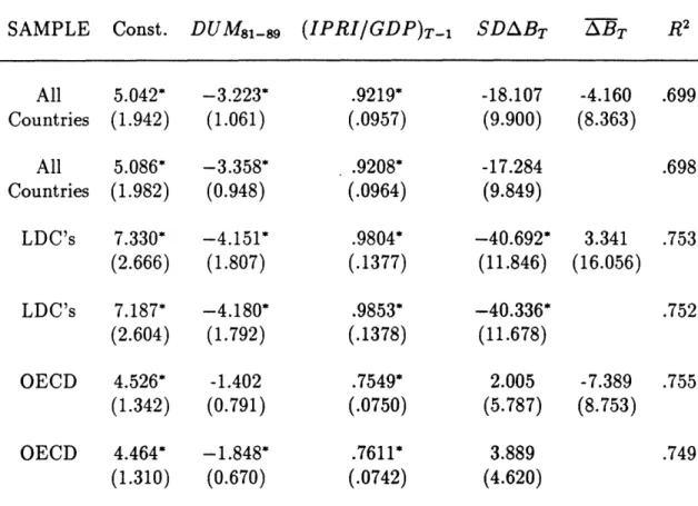
We have estimated the extent to which an increase in volatility can increase the required return for investment, but without a model that describes the distribution of returns across firms and its evolution through time we can say little about the effect of volatility on in-vestment itself. Furthermore, the theory tells us nothing about the relationship between volatility and investment in a steady-state equilibrium; it only tells us that an increase in volatility (or decrease in the drift rate) should be accompanied by an at least temporary de-crease in investment. To explore this, we divide our sample into three subperiods - 1962-71, 1972-80, and 1981-89 - and we calculate the sample mean and sample standard deviation of annual changes in b(t) for each. We then run panel regressions that relate the ratio of private investment to GDP to these measures of the drift and volatility.
The regressions are shown in Table 3. Note that in each case the number of observations is twice, and not three times, the number of countries (because the lagged investment-to-GDP ratio is an explanatory variable). Each equation includes a dummy variable for the 1981-89 subperiod to account for structural change or other variables that might affect investment. Regressions are run for the full sample of 29 countries, and then for the LDC's and OECD countries separately.
These regression results are mixed. They show a negative relationship between volatility and the rate of investment for the full sample, but the coefficients on SDABT are significant at the 5 percent level only for the LDC's, and have the wrong sign for the OECD countries. This is the case whether or not we include the drift variable, AB, on the right-hand side.
For the LDC's, the implied effect of volatility on the rate of investment is moderately important. The estimate of the coefficient on SDABT is about -40, which means that an increase in volatility of .05 corresponds to an 2 percent drop in the investment-to-GDP ratio for a period of several years. This is a significant drop given that for most countries the average ratios are less than 20 percent. The coefficient on SDABT is about half as large, however, for the full sample of 29 countries, and suggests that a .05 increase in the standard deviation of Ab(t) would lead to less than a 1 percent drop in the ratio of investment to GDP.
Volatility and Interest Rates.
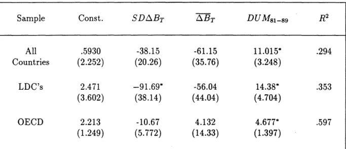
As an additional experiment, we can examine one of the general equilibrium implications of the theory. To the extent that investment is highly inelastic with respect to the interest rate (or even an increasing function of the interest rate), and savings is an increasing function of the interest rate, an increase in the volatility of b(t) should, at least in the short- to intermediate-term, reduce real interest rates. The reason is that an increase in the volatility of b(t) (or decrease in its drift rate) should at least temporarily shift the investment schedule to the left, thereby lowering interest rates. To test this we calculate the mean real interest rate for each of the three subperiods, and then run panel regressions to determine the dependence of the interest rate on SDAB and AB.
The regression results are shown in Table 4, first for the full sample of 29 countries, and then for LDC's and OECD countries separately. In each case the estimated coefficient of SDAB is negative as expected, and while it is statistically significant at the 5 percent level only for the LDC's, it is nearly significant for the full sample and for the OECD countries.
Note that the coefficient estimate of -38 for the full sample implies that a .05 increase in the standard deviation of Ab(t) leads to about a 200 basis point drop in the real interest rate. This is a very large effect, in part explained by the low interest-elalsticity of savings found in cross-country savings regressions for developing countries.1 5 This result must be viewed with caution, however, given the quality of the interest rate data for the LDC's. The estimated
coefficient for SDABT is only about one fourth as large for the OECD countries. Also, note that the coefficient on AB is always insignificant and has the wrong sign in two cases.
6. Sources of Volatility.
We have seen in Section 3 that the volatility of the log of the marginal profitability of capital is a summary statistic that describes all of the uncertainty relevant for investment decisions. A question that then arises is to what extent can this volatility be explained by various indicia of economic and political instability. For example, do the level or volatility of inflation, or the volatility of real exchange rates or interest rates help to explain the volatility of b(t)? And do indicia of political instability, such as the political variables used by Barro and Wolf (1991) in their recent study of determinants of growth, have much to do with the volatility of b(t)? These questions are impdrtant because if increases in the volatility.of b(t) even temporarily depresses investment, we would like to know what economic or political factors can cause such increases.
Table 5 shows simple correlations of SDAB with four economic indicia and seven political indicia of instability. The economic variables are the mean inflation rate (INF), the average annual standard deviation of the change in the inflation rate (SDAINF), the average annual standard deviation of the change in the real exchange rate (SDARER), and the average annual standard deviation of the change in the real interest rate (SDAR), in each case calculated over the full sample period for each country. The first political variable, PROB, is the annual probability of a change in government, as estimated from a probit model by Cukierman, Edwards, and Tabellini (1992), using data for the period 1948-1982. The other
political variables, ASSASS, CRISIS, STRIKE, RIOT, REVOL, and CONCHGE,
are the average number of assassinations, government crises, strikes, riots, revolutions, and constitutional changes per year over the period 1960-85, and are from Barro and Wolf (1991). The table shows correlations for the LDC's and for the OECD countries.
Only INF, SDAINF, and SDAR are significantly correlated with SDAB for both the LDC's and OECD countries. However, these variables are also highly correlated with each other. (For example, the correlation of INF with SDAINF is above .90.) Of the political
variables, only ASSASS, STRIKE, and RIOT are significantly correlated with SDAB, and then only for the LDC's.
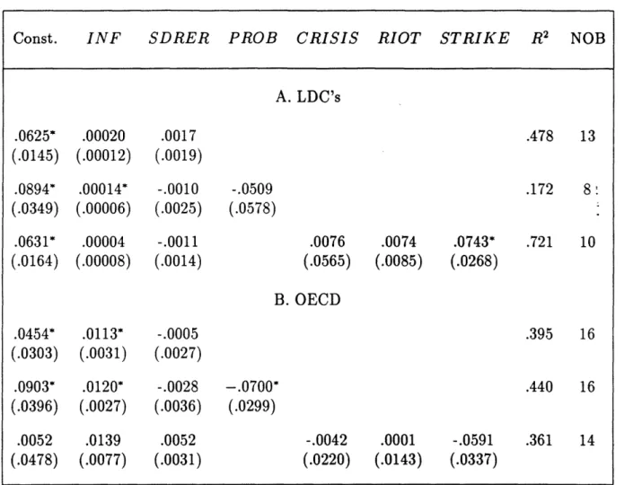
We ran a large set of cross-section regressions in order to explore the ability of these economic and political variables to "explain" the volatility of b(t). Table 6 shows only a small subset of these regressions, but the results are representative of our overall findings. Most important, the mean inflation rate is the only variable that is consistently significant as an explanator of SDAB. Although SDAINF and SDAR are individually correlated with SDAB, they are always insignificant when combined with INF in a regression. STRIKE is also significant in these regressions, but only for the LDC's. As long as INF is also in the regression, all of the other political variables are either insignificant and/or have the wrong sign. This is true for the LDC's, the OECD countries, or when the regressions are run over the full sample.
This suggests that strikes, riots, revolutions, and other forms of political turmoil and uncertainty (as measured by these indicia) may have little to do with uncertainty over the return on capital, and hence with investment. It may mean that as long as a government can control inflation - an indicator of overall economic stability, and from which exchange rate and interest rate stability tend to follow - it can limit the uncertainty that matters for investment. These results also raise doubts regarding recent results in the literature that relate indicia of political instability to growth. On the other hand, regressions of the sort shown in Table 6 have serious limitations. Aside from the very limited sample of countries, the most important limitation is our assumption that the relevant stochastic state variables follow Brownian motions, so that b(t) follows a controlled Brownian motion. This eliminates
"peso problems" as a source of uncertainty.
If we take these results at face value, they suggest that controlling inflation should be one of the most important intermediate objectives of policy. We explore this in more detail in the next section.
7.
Time Series Evidence.
best indicia of economic instability, and is associated with lower rates of capital formation. This seems to be particularly true at very high levels of inflation. In this section we explore the relationship between inflation and investment in more detail by examining a group of six OECD countries that have had relatively low inflation, and a group of high inflation countries, predominantly in Latin America. Our objective is to examine the robustness of the relationship between inflation and investment across countries with very different levels of inflation, and to explore possible nonlinearities in this relationship within each country group.
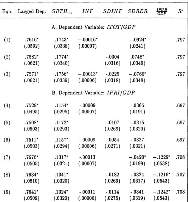
To do this, we study the relationship between year-to-year variation in different indicators of economic instability and the ratio of investment to GDP. This is important, because our use of nine-year averages in Section 5 may have concealed higher-frequency information. In this section we report on panel regressions that utilize annual data relating the ratio of investment to GDP (total and private) directly to three indicia of economic instability - the level and variability of inflation, and the variability of the real exchange rate. (Unfortunately annual data are not available for indicia of social and political instability.) This allows us to capture possible effects of economic instability on investment that may occur though channels other than the volatility of the marginal profitability of capital.'6
Of particular concern to us is inflation, which can affect investment in several ways: (i) High and volatile inflation may indicate an inability of the government to control the economy (see Fischer (1993)). As a consequence, government policies will be perceived by investors as unsustainable and hence risky, leading them to defer investing. (ii) High and volatile inflation is associated with greater volatility in the marginal profitability of capital, and with volatile relative prices (see Fischer and Modigliani (1978) and Fischer (1986)). (iii) Inflation amounts to a tax on real monetary balances. Hence if money and capital are complementary - through the production function or through cash-in-advance constraints - inflation and investment will be negatively correlated.'7
16Fischer (1986, 1991, 1993) discusses several channels through which inflation may affect growth and capital formation.