M
Maassssaacchhuusseettttss IInnssttiittuuttee ooff T
Teecchhnnoollooggyy
E
Ennggiinneeeerriinngg SSyysstteem
mss D
Diivviissiioonn
Working Paper Series
ESD-WP-2007-13
A
N
A
LGORITHM AND
M
ETRIC FOR
N
ETWORK
D
ECOMPOSITION FROM
S
IMILARITY
M
ATRICES
:
A
PPLICATION TO
P
OSITIONAL
A
NALYSES
Mo-Han Hsieh
1and Christopher L. Magee
21Engineering Systems Division Massachusetts Institute of Technology Cambridge, MA 02139, USA [email protected] 2Engineering Systems Division & Department of Mechanical Engineering, Massachusetts Institute of Technology, Cambridge, MA 02139, USA [email protected]
An Algorithm and Metric for Network Decomposition from
Similarity Matrices: Application to Positional Analyses
Mo-Han Hsieh a, *, Christopher L. Magee b
a Engineering Systems Division, Massachusetts Institute of Technology, Cambridge, MA 02139, USA. b Engineering Systems Division & Department of Mechanical Engineering, Massachusetts Institute of
Technology, Cambridge, MA 02139, USA. Abstract
We present an algorithm for decomposing a social network into an optimal number of structurally equivalent classes. The k-means method is used to determine the best decomposition of the social network for various numbers of subgroups. The best number of subgroups into which to decompose a network is determined by minimizing the intra-cluster variance of similarity subject to the constraint that the improvement in going to more subgroups is better than a random network would achieve. We also describe a decomposability metric that assesses how closely the derived decomposition approaches an ideal network having only structurally equivalent classes.
Three well known network data sets were used to demonstrate the algorithm and decomposability metric. These demonstrations indicate the utility of the approach and suggest how it can be used in a complementary way to the Generalized Blockmodeling.
* Corresponding author. Tel.: +1 617 577 5843; fax: +1 617 258 0485.
1. Introduction
In the network analysis literature, two lines of research have been pursued to develop methods of decomposing networks into meaningful subgroups (Wasserman and Faust 1994). These are: (1) research that seeks to identify cohesive subgroups (Frank 1995); and (2) research that seeks equivalent classes in a network (Lorrain and White 1971; Breiger, Boorman et al. 1975). While numerous methods have been proposed to conceptualize the idea of cohesive subgroups (including the algorithm recently proposed by Newman and Girvan (2004)), the recent efforts in social networks research have been on developing methods that identify equivalent classes.
Among the methods that identify equivalent classes, Batagelj et al. (1992) proposed to divide them into direct and indirect methods. An indirect method typically composes two major parts: (1) a definition of dissimilarity that is compatible with the selected type of equivalence (e.g. the corrected Euclidean-like dissimilarity (Burt and Minor 1983)) and (2) an algorithm that produces good clustering solutions (e.g. hierarchical clustering). The method is indirect in the sense that the relational information among vertices is first used to create a partition, and the partition is then evaluated with an explicit criterion function (Batagelj, Ferligoj et al. 1992). While most of these methods generate dissimilarity measures that are compatible with the selected types of equivalence, the clustering solutions based on these dissimilarity measures are generally not satisfying.
The often used method, CONCOR (Breiger, Boorman et al. 1975), is considered as having the aspects of both the indirect and direct method (Batagelj, Ferligoj et al. 1992). However, CONCOR procedure always splits a set of vertices into exactly two subsets. Repeated application of CONCOR would result in a series of subdivided bi-partitions of
the network. In this case, the partition outcome is at least partially determined by the procedure, not by the actual structure of the network (Schwartz 1977).
Indeed, the most recently developed approach in identifying equivalence subgroups is Generalized Blockmodeling (GBM) (Doreian, Batagelj et al. 2005). The method considers ideal blockmodels and uses optimization methods to fit them to empirical data. This direct method allows for use of context information in forming hypotheses and gives a criterion function (i.e. inconsistencies) that measures the fit of a specified blockmodel or decomposition structure to the actual data. GBM has been shown to give “better” decompositions of social network data based upon comparing inconsistencies (Batagelj, Ferligoj et al. 1992; Doreian, Batagelj et al. 2005). However, GBM does not have a clear definition of a “best” decomposition since (as noted in (Doreian, Batagelj et al. 2005)) hypotheses with more subgroups can always be found to lower the number of inconsistencies to zero. In many cases, this involves the decomposition to numerous singletons and of course in the limit one can trivially decompose a network to all singletons with no inconsistencies but also with no meaning. In other words, to become an inductive approach, GBM needs a criterion for stopping decomposition.
In this paper, we propose a new indirect method of partitioning a network into structural equivalence classes. Overall, the method consists of: (1) an unsupervised clustering method, in which vertices are assigned to clusters to minimize the intra-cluster variance of dissimilarity; (2) an approach that takes into consideration not only the dissimilarity between the pair of vertices but also the pair’s dissimilarities with all other vertices; (3) a quantitative stopping criteria for determining the number of subgroups that a network should be divided into to best represent its underlying equivalence structure. The method is seen as a companion to BGM offering additional insight in certain kinds of
studies (where inductive learning is useful) and having a similar limitation. The new method, at this point, is limited to structural equivalence basically because of the lack of valid dissimilarity measures for the potentially more interesting types of equivalence such as “regular” equivalence.
The paper presents the new method for finding structural equivalence classes and its application to ideal structurally equivalent networks in Section 2. In section 3, we develop a normalized decomposability metric for assessing how close non-ideal networks are to the ideal networks found by our (or any) decomposition methodology. Application of our method including the decomposability metric to three known social networks is presented in Section 4. Brief concluding remarks are given in Section 5.
2. A New Method for Finding Structural Equivalence Classes
The method starts with any dissimilarity measure of vertices that is compatible with structural equivalence. For an n-node network, these dissimilarity measures can be arranged in an n by n matrix, whose entries give the dissimilarity between the row vertices i and the column vertices j. Hierarchical clustering generates the hierarchy of vertices by using these measures and different definitions of dissimilarity between the new clusters. Our method treats the n by n dissimilarity matrix as n data points in the
n-dimensional space that we wish to partition. That is, we read row i of the dissimilarity
matrix as the n-dimensional coordinates of the ith data points. Since the dissimilarity matrix is symmetric, the coordinates can also be read as the column elements.
With n data points in the n-dimensional space, we then repeatedly apply the k-means method to partition the n data points into k=2 to k=n clusters. Lloyd’s k-means algorithm (Lloyd 1982) begins with a set of k reference points which are randomly
selected from the data set. All of the data points are partitioned into k clusters by assigning each point to the cluster of its closest reference point. In each iteration, the centroid for each cluster is calculated. A new partition is then made by using those centroids as reference points for all of the data points. It has been proven (Bottou and Bengio 1995) that the iterative process will eventually converge to a configuration where each data point is closer to the reference point of its cluster than to any other reference point and each reference point is the centroid of its cluster. Since different initial reference points can generate different partitions, multiple sets of initial points are used to evaluate whether the obtained partition has approached its minimum sum of intra-cluster distances. Information about the k-means method and its many variations can be found in (Kaufman and Rousseeuw 2005).
For each round of the k-means method that partitions the n data points into k clusters, we have the sum of the within cluster points-to-centroid distances as
2 1
∑ ∑
= ∈ − = k i j S j i k ix
c
D
(1)where Si (i=1,2,…,k) is the cluster and ci is the centroid or mean point of all of the
data points xj in cluster Si.
In the process of decomposing the network into more subgroups (i.e. as k increases),
Dk gradually decreases as more centroids are generated. A smaller Dk is desirable
because we want a partition that has a smaller intra-cluster variance. Dk is zero when
all of the equivalent classes (including singletons) have been identified by at least one centroid. For ideal networks having only structurally equivalent classes, an algorithm could stop further partitioning the network when Dk is zero. However, for most real
individually identified as unique equivalent classes. In the case of k = n, Dk is always
zero because every node is identified as itself an equivalent class. The result of identifying a great number of singletons is relatively meaningless since it does not inform us about the underlying structure of the network. To avoid generating an excessive number of classes for real networks, a quantitative criterion must be designed to appropriately stop further decomposition of the networks.
For any assigned number of subgroups, the k-means method seeks to minimize Dk
with the same number of centroids. Because nodes of the same equivalent class have the same coordinates, a lower Dk can be obtained by first grouping them with centroids.
Therefore, if a network has equivalent classes, Dk decreases significantly with newly
added centroids until every equivalent class has been identified by at least one centroid. The decrease of Dk slows down with larger k when singletons start to appear as classes.
To some extent, these singletons, with their unique linkage patterns, are similar to randomly wired nodes in a network. Therefore, the gradual decrease of Dk during the
generation of singletons is similar to that of a random network. Thus, we stop further dividing a network into additional subgroups by comparing the decrease of Dk with that of
a random network with the same size and density. In other words, we stop further partitioning the network if the decrease of its Dk from k to k + 1 is less than that of a
comparable random network. We thus define a fitness index as simply
D
D
F
real k random k k= − (2) where random kD is the sum of intra-cluster point-to-centroid distances of the random
network and real k
of k, and the corresponding k represents the appropriate subdivision of the network because further subdivision is only reducing Dk at random (or less than random) rates.
The nodes belonging to the k different clusters then form the equivalent classes of the network.
In theory, our method works for all of the ideal networks having only structurally equivalent classes because nodes of the same equivalent class cause a larger decrease of the sum of intra-cluster point-to-centroid distances than nodes that belong to no equivalent class. This also works in practice as we have tried the algorithm for a variety of ideal networks and the algorithm identifies the correct subgroups for all of them. However, there are easy and difficult cases of using the fitness index to identify the right number of classes that the network has. The difficult cases are the networks whose decrease of the sum of intra-cluster point-to-centroid distances is only slightly higher than that of the random network. Figure 1 shows two sets of comparison between these difficult and easy cases. Each fitness value in the figure is normalized between zero and one so that we can compare their resolution. Figure 1(a) shows the fitness index for two ideal networks with the same minimum equivalent class size (i.e. C=5) but different network size (i.e. n=25 and 100). As shown in the figure, it is easier to identify the peak of fitness index for the network with smaller size because the fitness index has better resolution. Figure 1(b) shows the fitness index for two ideal networks with the same network size (i.e. n=50) but different minimum equivalent class size (i.e. C=2 and 10). As shown in the figure, the network with larger minimum equivalent class size has better resolution, thus makes it easier to identify the peak of fitness index. In general, networks having small equivalent classes and larger network sizes are the difficult cases of using the fitness index to identify the right number of classes that the network has.
Nonetheless, the method identifies the correct ideal network in all cases. 0.0 0.1 0.2 0.3 0.4 0.5 0.6 0.7 0.8 0.9 1.0 1 5 9 13 17 21 25 29 33 37 41 45 49 k Fi
tness Index (no
rm a liz e d w it h max. f it n es s) n=25, C=5 n=100, C=5 (a) 0.0 0.1 0.2 0.3 0.4 0.5 0.6 0.7 0.8 0.9 1.0 1 5 9 13 17 21 25 29 33 37 41 45 49 k Fi
tness Index (no
rm a liz e d w it h max. f it n es s) n=50, C=10 n=50, C=2 (b)
Figure 1. (a) Fitness index for ideal networks with the same minimum equivalent class size (i.e. C=5) but different network size (i.e. n=25 and 100). (b) Fitness index for two ideal networks with the same network size (i.e. n=50) but different minimum equivalent class size (i.e. C=2 and 10).
3. Measuring the decomposability of a network
By applying our class finding algorithm, networks are divided into subgroups that correspond to their underlying equivalent structures. However, we want to differentiate among networks whose subgroups are not all ideal equivalent classes. In this case, we define perfect decomposability of a network as that achieved when a network is composed of only equivalent classes.
Having a normalized objective measurement of decomposability is useful. For example, we can compare two networks and determine which network is more similar to an ideal network having only equivalent classes. Lower decomposability can be used to infer that the suggested decomposition is more forced and thus should be cautiously utilized in further analysis. Moreover, if other variables (or time series data) are known, the change of decomposability with the variables (or with time) affecting the network can be found. This can allow one to find how various variables influence the structural roles in a given network or a variety of different networks.
To determine the normalized decomposability of a network, we construct an objective measurement that places networks with only equivalent classes at one end and those without any equivalent class at the other. We use the sum of intra-cluster distance,
Dk, of Eq. (1), to quantify the similarity between a real network and an ideal network.
For an ideal network having only equivalent classes, its sum of intra-cluster distance,
Dideal, equals to zero. This is because every member of the same equivalent class,
when viewed as a node in the multidimensional space, has the same coordinates. Therefore, their intra-cluster distances equals to zero and the sum of these distances,
Dideal, equals to zero.
In addition to the value of Dideal , we want the upper bound of the sum of intra-cluster
distance, Dmax(n,k), for networks having n nodes and k clusters. With the lower bound,
Dideal=0, and the upper bound, Dmax(n,k), we can thus obtain the normalized
decomposability, Q, for the network as
) , max( ) , max( 1 1 k n k ideal k n ideal k D D D D D D Q = − − − − = (3)
which defines Q as 1 for perfect decomposability and 0 for Dk = Dmax(n,k) which is
equivalent to no decomposability. To obtain the upper bound, Dmax(n,k), we are seeking a
network that has the maximum possible value of Dk while having the same size and is
divided into the same number of clusters as that of the ideal network. To obtain the upper bound of Dk, we apply the Monte Carlo method to obtain an approximate solution
for the network with size, n, and number of clusters, k. By using the corrected Euclidean-like dissimilarity (Burt and Minor 1983) as the dissimilarity measure for structure equivalence, Table 1 shows some examples of Dmax(n,k) (with three significant
Size of Network (n) 6 7 8 9 10 11 12 13 14 15 2 21.3 32.2 44.6 60.3 76.7 96.4 120 146 168 196 3 14.3 23.2 33.5 46.8 61.7 77.4 97.2 121 144 168 4 8.39 16.4 26.5 36.8 49.5 65.1 82.8 102 125 146 Number of Clusters (k) 5 4.51 10.5 17.8 27.6 41.4 54.6 68.8 86.9 106 131
Table 1. Dmax for network with different sizes and number of clusters
In the table, the maximum possible Dk for a 9-node network, for example, divided into
three clusters is Dmax(n,k)=Dmax(9,3)=46.8. With this information, we consider three 9-node
networks as shown in Figure 2.
Network 1 and its adjacency matrix 1 2 3 4 5 6 7 8 9 1 0 1 1 0 0 0 0 0 1 2 1 0 1 0 0 0 0 0 0 3 1 1 0 0 0 0 0 0 0 4 0 0 0 0 1 1 0 0 0 5 0 0 0 1 0 1 0 0 0 6 0 0 0 1 1 0 0 0 0 7 0 0 0 0 0 0 0 1 1 8 0 0 0 0 0 0 1 0 1 9 0 0 0 1 0 0 1 1 0 Network 2 and its adjacency matrix
1 2 3 4 5 6 7 8 9 1 0 1 1 0 0 0 0 0 1 2 1 0 1 0 0 0 0 0 0 3 1 1 0 0 0 0 0 0 0 4 0 0 0 0 1 1 0 0 0 5 0 0 0 1 0 1 0 0 0 6 0 0 0 1 1 0 0 0 0 7 1 0 0 0 0 0 0 1 1 8 0 0 0 0 0 0 1 0 1 9 0 0 0 1 0 0 1 1 0 Network 3 and its adjacency matrix
1 2 3 4 5 6 7 8 9 1 0 1 1 0 0 0 0 0 1 2 1 0 1 0 0 0 1 0 0 3 1 1 0 0 0 0 0 0 0 4 0 0 0 0 1 1 0 1 0 5 0 0 0 1 0 1 0 0 0 6 0 0 0 1 1 0 0 0 0 7 1 0 0 0 0 0 0 1 1 8 0 0 0 0 0 0 1 0 1 9 0 0 0 1 0 0 1 1 0
Figure 2. Network 1, 2, and 3 and their adjacency matrixes.
3 2 1 4 5 6 7 9 8 3 2 1 4 5 6 7 9 8 3 2 1 4 5 6 7 9 8
Note that the only difference between Network 1 and Network 2 is the directed link from node 7 to node 1. Network 3 differs from Network 2 by its additional links from node 2 to node 7 and from node 4 to node 8. The result of applying our class finding algorithm to Network 1 and Network 2 shows that the two networks are divided into the same three clusters (i.e. node 1, 2, and 3, node 4, 5, and 6, and node 7, 8, and 9). Moreover, we obtain Dk = D3 = 8.71 for Network 1 and D3 = 11.2 for Network 2. Therefore, the
decomposability for Network 1 is 81 . 0 8 . 46 / 71 . 8 1 1 ) 3 , 9 max( 3 1= − = − = D D Q
and the decomposability for Network 2 is 76 . 0 8 . 46 / 2 . 11 1 1 ) 3 , 9 max( 3 2 = − = − = D D Q .
Similarly, our class finding algorithm tells us that Network 3 should be divided into still the same three clusters. With its sum of intra-cluster distance, D3, equals to 16.2, we obtain
its decomposability as 65 . 0 8 . 46 / 2 . 16 1 1 ) 3 , 9 max( 3 3 = −D = − = D Q .
With Network 1 having the highest decomposability and Network 3 having the lowest, the decomposability metric confirms what visual inspection tells us; Network 2 is closer to the ideal network than is Network 3 but is further from ideal than is Network 1.
Since the decomposability can be viewed as a measure of deviation of real networks from ideal networks that contain only equivalent classes, we explored the relationship between a network’s decomposability and its deviation from an ideal network. To do this, we examine the decomposability of 10,000 pseudo real networks generated from
randomly perturbing1 all possible linkages of ideal networks (i.e. adding or removing links) with six different percentages. Ideal networks with sizes between 30 and 60 were sampled. Furthermore, we sample ideal networks with the assumption that the number of classes for each network is normally distributed and the size of each class within a network is also normally distributed. Since real networks typically have very low density, we only sample ideal networks with density lower than 0.2.
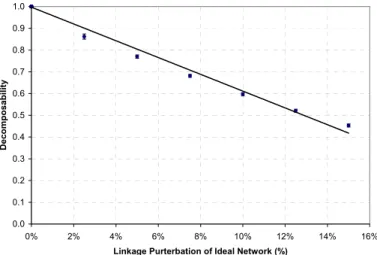
Figure 3 shows the average decomposability of the pseudo real networks (with one standard deviation also plotted) versus their percentage of linkage perturbation from ideal networks. As shown in the figure, the linear relationship between the two has an R-square value of 0.99. In other words, the more a network deviates from any ideal network (i.e. with higher percentage of linkage perturbation), the lower its decomposability is.
With this result, we can calculate the deviation of our previous three networks. Referring to Figure 3, the decomposability of Network 1, 2, and 3 (calculated above) are equivalent to 4.8%, 6.1%, and 8.9% linkage perturbation of their underlying ideal network. It should be noted that real networks are less likely to preserve their underlying structure with increasing percentage of linkage perturbation. Indeed, by extrapolating the linear relationship shown in Figure 3, the upper limit of linkage perturbation for a real network to preserve any vestige of its original structure is about 25%. In this case, the corresponding decomposability is zero. However, even for non-zero decomposability, we should proceed with some extra caution in trusting the decomposition as decomposability falls.
1 The perturbation can be viewed as arising from an error in observation or arising because real social relationships
0.0 0.1 0.2 0.3 0.4 0.5 0.6 0.7 0.8 0.9 1.0 0% 2% 4% 6% 8% 10% 12% 14% 16%
Linkage Purterbation of Ideal Network (%)
D e co mpos ab il it y
Figure 3. Decomposability versus linkage perturbation of ideal network 4. Application of the Method
In the previous sections, we propose a method for clustering nodes of networks into meaningful equivalent classes and a decomposability metric to quantify a network’s level of linkage perturbation from its underlying ideal network. Because our method can identify the number of classes for any ideal network having only structurally equivalent classes, in this section we test our method and the decomposability metric with three examples of real networks.
The multiplex ties among workers in an office reported by Thurman (1979) is used as the first example to evaluate our method. The dataset is comprised of the social relationship and the authoritative relationship among the 15 workers. The social network is shown in Figure 4(a), and the organizational chart is shown in Figure 4(b).
(a)
President
Pete
Minna Katy Bill Ann Andy Emma
Peg Rose Tina Mike Marry
Amy Lisa
(b)
Figure 4. (a) The social network and (b) the organizational chart of Thurman office data.
By applying our method to first partition the authoritative network into k=2 to k=15 subgroups, the sum of intra-cluster point-to-centroid distances as a function of k is obtained and is shown in Figure 5(a) as dark gray bars. To obtain the fitness index, we need the comparable sum of any sampled random network that has the same size and density as the authoritative network. This sum of intra-cluster point-to-centroid distances as a function of k is shown in Figure 5(a) as light gray bars. The fitness index generated by subtracting the one of the authoritative network from that of the random network is shown in Figure 5(b).
0 20 40 60 80 100 120 1 2 3 4 5 6 7 8 9 10 11 12 13 14 15 k S u m of i n tr a-cl uster poi nt-to-centr oi d di st an ces Random Network Authoritative Network (a) 0 20 40 60 80 100 120 1 2 3 4 5 6 7 8 9 10 11 12 13 14 15 k S u m of in tr a-c lus ter poi nt -to-centr oi d di st ance s Fitness Index (b)
Figure 5. (a) The sum of intra-cluster point-to-centroid distances of Thurman’s office authoritative network (dark gray bars) and that of the random network with the same size and density (light gray bars). (b) The
fitness index of Thurman’s office authoritative network.
As shown in Figure 5(b), the fitness index has its maximum at k=5, which by our method indicates that the best decomposition of the network is into five equivalent classes. These equivalent classes are: (1) the President and Pete, (2) Katy, Bill, Ann, and Andy, (3) Minna, Amy, and Lisa, (4) Peg, Rose, Tina, Mike, and Marry, and (5) Emma herself. This partition corresponds well with the organizational chart shown in Figure 4(b). With the same procedure, we partition the social network into k=2 to k=15 subgroups, we first obtain the sum of intra-cluster point-to-centroid distances of the social network and the random network as shown in Figure 6(a). The fitness index thus obtained is shown in Figure 6(b). 0 20 40 60 80 100 120 140 160 180 1 2 3 4 5 6 7 8 9 10 11 12 13 14 15 k Su m o f i n tr a-c lu ster p o in t-t o -cen tr o id d istan ces Random Network Social Network (a) -20 0 20 40 60 80 100 120 1 2 3 4 5 6 7 8 9 10 11 12 13 14 15 k S u m of in tra -cl uste r poi nt-t o-centroi d d istances Fitness Index (b)
Figure 6. (a) The sum of intra-cluster point-to-centroid distances of Thurman’s office social network (dark gray bars) and that of the random network with the same size and density (light gray bars). (b) The fitness index of Thurman’s office social network.
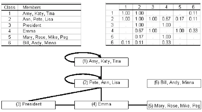
The fitness index shown in Figure 6(b) has the maximum at k=6, indicating that the best decomposition is into six equivalent classes. Figure 7 shows these six classes and the block model as revealed by using our method.
Figure 7. Class members, block density, and image graph of the Thurman social network
As shown in Figure 7, the first class includes Amy, Katy, and Tina, and the second class includes Ann, Pete, and Lisa. There is strong interaction within and between the two classes. What differentiates them is that the second class has strong interaction with the President. According to Thurman (1979), Pete is characterized as the center of a social circle that included Lisa, Katy and Amy. Ann arrived under the sponsorship of Pete, and Lisa has the ear of the President (Thurman 1979). It is worth noticing that the fourth class comprises only Emma, who has strong interaction with the President, the members of the second class, and the members of the fifth class. According to Thurman (1979), she plays a special role in the social network.
With the network size equals to 15 and the number of subgroups equals to five for the authoritative network and six for the social network, we have the upper bound of the sum of intra-cluster distance, Dmax(15,5) =130.71 and Dmax(15,6) =113.07. By using
0.95 and 0.65 respectively. While both of these decomposabilities are reasonably high,
the authoritative network is much more similar to an ideal network in terms of its equivalence structures and thus is more reliably discussed in terms of this structure.
By using the relationship between the decomposability and the linkage perturbation of the ideal network shown in Figure 3, we can infer that the authoritative network is about 1.2% linkage perturbation from the ideal network and the social network is about 8.9% linkage perturbation from the ideal network. This strongly indicates that the authoritative network is more solidly linked to the data but the inferred equivalence structure of the social network might be substituted for easily with more observation or slight changes in interaction patterns.
The inter-organizational Search and Rescue (SAR) network created after a disaster in Kansas (Drabek 1981) is used as the second example to demonstrate the use of the new method. The SAR network has 20 organizations. The dichotomized communication data among these organizations are shown in Table 2.
A B C D E F G H I J K L M N O P Q R S T
Osage County Sheriff's Department A 0 1 1 0 1 1 1 0 1 0 1 0 0 0 1 1 1 0 0 1
Osage County Civil Defense Office B 1 0 1 0 1 1 1 0 1 0 0 0 0 1 0 1 1 0 0 0
Osage County Coroner's Office C 1 0 0 1 1 1 0 0 1 0 1 0 0 0 0 0 1 0 0 0
Osage County Attorney's Office D 1 1 1 0 1 1 1 0 1 0 0 0 0 1 0 0 0 0 0 0
Kansas State Highway Patrol E 1 0 1 1 0 1 1 0 0 0 1 1 1 1 0 1 1 0 0 1
Kansas State Parks and Resources Authority F 1 0 1 1 1 0 1 0 1 0 1 1 0 1 0 0 0 0 0 0
Kansas State Game and Fish Commission G 1 0 1 1 1 1 0 0 1 1 0 0 0 0 0 1 0 0 0 0
Kansas State Department of Transportation H 1 1 0 0 1 0 0 0 0 1 0 0 0 0 0 0 0 0 0 0
U.S. Army Corps of Engineers I 1 0 1 0 1 1 1 0 0 0 1 1 0 0 0 0 1 0 0 0 U.S. Army Reserve J 1 0 0 0 1 0 0 0 0 0 0 0 0 0 0 0 0 0 0 0
Crable Ambulance K 1 0 1 0 1 1 1 0 1 0 0 0 0 0 0 0 0 0 0 0
Franklin County Ambulance L 1 0 0 0 1 0 1 0 0 0 0 0 0 0 0 0 1 0 0 0
Lee's Summit Underwater Rescue Team M 1 0 0 0 1 0 0 0 0 0 0 0 0 0 0 0 0 0 0 0
Shawney County Underwater Rescue Team N 1 0 1 0 1 1 1 0 1 0 0 0 1 0 0 0 1 1 0 1
Burlingame Police Department O 1 0 1 1 1 1 1 0 1 1 1 1 1 1 0 1 1 1 0 1
Lyndon Police Department P 1 1 0 0 1 1 1 0 0 0 1 1 0 0 0 0 0 0 0 0
American Red Cross Q 1 1 1 0 1 1 1 0 1 1 0 0 0 1 0 0 0 0 0 0
Topeka Fire Department Rescue #1 R 1 0 0 0 1 0 0 0 0 0 0 0 1 1 0 0 0 0 0 0
Carbondale Fire Department S 1 1 0 0 1 1 1 0 1 0 0 0 0 0 0 0 1 0 0 0
Topeka Radiator and Body Works T 1 0 0 0 1 0 0 0 0 0 0 0 0 0 1 1 1 0 0 0
Table 2. Kansas SAR Inter-organizational Network
network into five clusters as: 1. Authority position: {A, E}. 2. Primary support: {C, F, G, I, K}. 3. Critical resources: {D, L, N}.
4. Secondary support, 1: {M, O, P, Q, R, T}. 5. Secondary support, 2: {B, H, J, S}.
While these five subgroups are potentially useful in understanding this network, Doreian et al. (2005) showed that this partition has 79 inconsistencies when examined with their GBM criterion function for structural equivalence. They found a five-cluster alternative that has only 57 inconsistencies (indicating the weakness of CONCOR discussed in the Introduction to this paper):
1. Authority: {A, E}.
2. Bodies and Survivors: {C, F, G, I}. 3. Infrastructure: {B, D, K, N, P, Q}.
4. Primary Rescue Operators: {H, J, L, M, R, S, T}. 5. Secondary Rescue Operators: {O}.
Applying the method presented in this paper to find the structural equivalence classes of the SAR network, we again partition the network into k=2 to k=20 subgroups. The sum of intra-cluster point-to-centroid distances of the SAR network and that of the random network with the same size and density is shown in Figure 8(a). The fitness index is shown in Figure 8(b).
0 50 100 150 200 250 300 350 1 2 3 4 5 6 7 8 9 10 11 12 13 14 15 16 17 18 19 20 k S u m of int ra -c lus te r point-to-c e n tr o id dis ta n ce s Random Network SAR Network (a) 0 20 40 60 80 100 120 1 2 3 4 5 6 7 8 9 10 11 12 13 14 15 16 17 18 19 20 k S u m o f in tra -c lu ste r p o in t-to -c en tro id d ista n ce s Fitness Index (b)
Figure 8. (a) The sum of intra-cluster point-to-centroid distances of the SAR network and random network with the same size and density. (b) The fitness index of the SAR network.
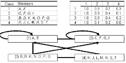
The fitness index shown in Figure 8(b) has its maximum at k=4, indicating that the best decomposition is into four equivalent classes. Figure 9 shows these four classes and the block model as revealed by using our method.
Figure 9. Class members, block density, and image graph of the SAR network
As shown in figure 9, our partition differs from that of Doreian et al. (2005) only in that ours combines their two classes, {B, D, K, N, P, Q} and {O}, into one class. By using the criterion function for structural equivalence proposed by Doreian et al., our partition has 64 inconsistencies, which is considerably better than the 79 for the five
subgroups suggested by CONCOR but seven more than the five subgroup partition proposed by Doreian et al using their direct method. Since more subgroups will decrease the inconsistencies, we examine the five-class decomposition of our method: 1. {A, E},
2. {C, F, G, I}, 3. {B, N, O}, 4. {D, K, P, Q},
5. {H, J, L, M, R, S, T}.
This partition breaks the third class of our four-class partition into two classes as {B,
N, O} and {D, K, P, Q}. This decomposition has the same 57 inconsistencies as that of
the different partition of Doreian et al. when examined with their criterion function. Thus, our method appears more effective than CONCOR and relative to GBM is capable of finding interesting decompositions that are worthy of consideration along with various hypotheses arrived at by other information.
With the network size equal to 20 and the number of subgroups equals to four for our first partition and five for the other partitions., we have the upper bound of the sum of intra-cluster distance, Dmax(20,4) =298.51 and Dmax(20,5) =271.56. With these upper
bounds, our first partition has decomposability of 0.42, which is greater than the five subgroup partition of Drabek et al (i.e. 0.41) and slightly lower than that of the partition of Doreian et al (i.e. 0.44) and that of our five subgroup partition (i.e. 0.45). We feel it is more important to notice that the decomposability of 0.42 is about 15% perturbation from the ideal network. With this high percentage of linkage perturbation, we should be cautious when using any of the inferred equivalence structures of the SAR network. Conversely, we can use the low decomposability of the SAR network data and the lack of clarity about structure derived from that data to support the contention that
communication structures were weak in this instance (Drabek 1981).
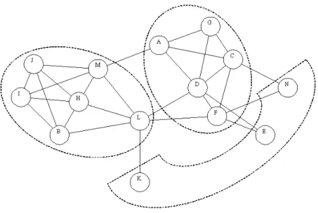
Our third example is the political actor network reported by Doreian and Albert (1989). In this network, the nodes are the prominent political actors in a local community and the links represent “strong political ally” among the actors. Figure 10 shows the three-class partition obtained by using CONCOR in the original analysis.
Figure 10. Political actor network with 32 inconsistencies and the decomposability of 0.42.
According to Doreian et al. (2005), this partition has 32 inconsistencies when examined with the GBM criterion function for structural equivalence. They proposed a three-cluster alternative shown in Figure 11 that has only 26 inconsistencies.
Figure 11. Political actor network with 26 inconsistencies and the decomposability of 0.37.
By applying our method to find the structural equivalence classes of the network, maximization of the fitness index indicates that the network is best decomposed into four equivalent classes. The four-class partition is shown in Figure 12. When examined with the criterion function proposed by Doreian et al. (2005), it has 25 inconsistencies, which is one less than that of the partition shown in Figure 11.
Since reduced inconsistency is expected with more subgroups, we also explore the 3 subgroup solution from the inductive method. In this case, our method suggests the
same partition as that shown in Figure 10. Though it has more inconsistencies than
that of the partition shown in Figure 11, the former has decomposability of 0.42 that is higher than 0.37 of the latter. This result clearly shows that our four-class partition, with 25 inconsistencies and decomposability of 0.49, has the best quality in terms of both the criterion function and the decomposability. However, the relatively low decomposability of this network indicates that any of these interpretations is open to change if more or slightly modified data was obtained about these networks. Alternatively, the relatively low decomposability indicates that the structure is significantly deviated from any ideal model and thus the political actor network is relatively weakly structured.
5. Conclusion and Discussion
The algorithm described in this paper appears to bring additional theoretical utility to existing methodology for decomposing networks into structurally equivalent subgroups. The theoretical advantage is its ability to find all ideal structurally equivalent subgroups but yet has an objective stopping criterion for continuing decomposition of non-ideal networks. The algorithm also appears to bring additional practical utility to existing tools such as the Generalized Blockmodeling by suggesting different decompositions of clear comparative merit to even well-studied examples as shown in Section 4.
When the algorithm is used in combination with Generalized Blockmodeling, one might obtain the advantages of combining inductive and deductive approaches. For example, with new data sets, one could start with finding the decompositions inductively (best and near best) and by in-context study of these possibly arrive at a new hypothesis
to test by various criteria. In general, applying both methods seems to be appropriate in all cases because the results in Section 4 indicate they can deliver slightly different and yet interesting decompositions. In addition, the examples show the potential merit of using our metric for decomposability. The metric provides an objective assessment of the normalized decomposability of various networks (and for various decompositions).
The algorithm can be used in combination with the widely applied hierarchical clustering. For structural equivalence or for any other similarity measures, the method described here can quickly suggest a best decomposition into a specific set of block models and roles. This can be compared with the suggested hierarchy and provide additional structural information of interest. Interesting future research could include: (1) application of the algorithm in biological, economic and engineering system classification problems and (2) comparison of the results of this algorithm with the one developed by Newman and Girvan based upon cohesive subgroups in a wide variety of network types.
References
Batagelj, V., A. Ferligoj, et al. (1992). "Direct and Indirect Methods for Structural Equivalence." Social Networks 14(1-2): 63-90.
Bottou, L. and Y. Bengio (1995). Convergence properties of the k-means algorithm. Adv. in Neural Info. Proc. Systems. G. Tesauro and D. Touretzky. Cambridge MA, MIT Press. 7: 585–592.
Breiger, R. L., S. A. Boorman, et al. (1975). "Algorithm for Clustering Relational Data with Applications to Social Network Analysis and Comparison with
Multidimensional-Scaling." Journal of Mathematical Psychology 12(3): 328-383. Burt, R. S. and M. J. Minor (1983). Applied network analysis: a methodological
introduction. Beverly Hills, Sage Publications.
Doreian, P. and L. H. Albert (1989). "Partitioning Political Actor Networks: Some Quantitative Tools for Analyzing Qualitative Networks." Journal of Quantitative
Anthropology(1): 279-291.
Doreian, P., V. Batagelj, et al. (2005). Generalized blockmodeling. Cambridge, U.K.; New York, Cambridge University Press.
Drabek, T. E. (1981). Managing multiorganizational emergency responses: emergent search and rescue networks in natural disaster and remote area settings. [Boulder, Colo.], Institute of Behavioral Science, University of Colorado.
Frank, K. A. (1995). "Identifying Cohesive Subgroups." Social Networks 17(1): 27-56. Kaufman, L. and P. J. Rousseeuw (2005). Finding groups in data: an introduction to
cluster analysis. Hoboken, N.J., Wiley.
Lloyd, S. P. (1982). "Least-Squares Quantization in Pcm." Ieee Transactions on Information Theory 28(2): 129-137.
Lorrain, F. and H. C. White (1971). "Structural equivalence of individuals in social networks." Journal of Mathematical Sociology(1): 49-80.
Newman, M. E. J. and M. Girvan (2004). "Finding and evaluating community structure in networks." Physical Review E 69(2): -.
Schwartz, J. E. (1977). An examination of CONCOR and related methods for blocking sociometric data. Sociological Methodology. D. R. Heise. San Francisco, Jossey-Bass: 255-282.
Thurman, B. (1979). "In the Office - Networks and Coalitions." Social Networks 2(1): 47-63.
Wasserman, S. and K. Faust (1994). Social network analysis: methods and applications. Cambridge; New York, Cambridge University Press.