Temporal disaggregation of satellite-derived monthly precipitation estimates and the resulting propagation of error in partitioning of water at the land surface

HAL Id: hal-00304569

https://hal.archives-ouvertes.fr/hal-00304569

Submitted on 1 Jan 2001

HAL is a multi-disciplinary open access archive for the deposit and dissemination of sci-entific research documents, whether they are pub-lished or not. The documents may come from teaching and research institutions in France or abroad, or from public or private research centers.

L’archive ouverte pluridisciplinaire HAL, est destinée au dépôt et à la diffusion de documents scientifiques de niveau recherche, publiés ou non, émanant des établissements d’enseignement et de recherche français ou étrangers, des laboratoires publics ou privés.

precipitation estimates and the resulting propagation of

error in partitioning of water at the land surface

S.A. Margulis, D. Entekhabi

To cite this version:

S.A. Margulis, D. Entekhabi. Temporal disaggregation of satellite-derived monthly precipitation esti-mates and the resulting propagation of error in partitioning of water at the land surface. Hydrology and Earth System Sciences Discussions, European Geosciences Union, 2001, 5 (1), pp.27-38. �hal-00304569�

Temporal disaggregation of satellite-derived monthly precipitation

estimates and the resulting propagation of error in partitioning of

water at the land surface

Steven A. Margulis and Dara Entekhabi

Ralph M. Parsons Laboratory, Department of Civil and Environmental Engineering, Massachusetts Institute of Technology, Cambridg e, MA 02139, USA email for corresponding author: margulis@MIT.edu

Abstract

Global estimates of precipitation can now be made using data from a combination of geosynchronous and low earth-orbit satellites. However, revisit patterns of polar-orbiting satellites and the need to sample mixed-clouds scenes from geosynchronous satellites leads to the coarsening of the temporal resolution to the monthly scale. There are prohibitive limitations to the applicability of monthly-scale aggregated precipitation estimates in many hydrological applications. The nonlinear and threshold dependencies of surface hydrological processes on precipitation may cause the hydrological response of the surface to vary considerably based on the intermittent temporal structure of the forcing. Therefore, to make the monthly satellite data useful for hydrological applications (i.e. water balance studies, rainfall-runoff modelling, etc.), it is necessary to disaggregate the monthly precipitation estimates into shorter time intervals so that they may be used in surface hydrology models. In this study, two simple statistical disaggregation schemes are developed for use with monthly precipitation estimates provided by satellites. The two techniques are shown to perform relatively well in introducing a reasonable temporal structure into the disaggregated time series. An ensemble of disaggregated realisations was routed through two land surface models of varying complexity so that the error propagation that takes place over the course of the month could be characterised. Results suggest that one of the proposed disaggregation schemes can be used in hydrological applications without introducing significant error.

Keywords: precipitation, temporal disaggregation, hydrological modelling, error propagation

Introduction

A major focus of large scale hydrological studies is the determination of the coupled water and energy balances at the land surface where atmospheric forcing is partitioned based on the surface characteristics. Precipitation is the key input quantity due to its role as a forcing field. In terms of the water balance, precipitation is partitioned at the surface into infiltration and surface runoff based on the soil moisture state. The infiltrated water is then redistributed throughout the unsaturated zone where it may later be returned to the atmosphere through evapotranspiration or lost to the groundwater system. While much of the focus of surface hydrological modelling is directed at the partitioning of water and energy at the surface, the accurate specification of the forcing, especially at large scales, is by no means a trivial matter.

Historically, estimates of precipitation have been obtained largely by using a network of ground-based rain gauges. While rain gauges remain the standard source of precipitation estimates, there are several problems and limitations

associated with them. One of the primary problems is that they provide point measurements of a quantity that varies significantly in both space and time. Spatial averaging techniques are often used to provide large scale estimates; however, significant biases are possible due to the undersampling of precipitation spatial fields. These errors can be especially large in areas where the gauge network is sparse. There are also inherent problems associated with under-capture at individual rain gauges due to local wind effects around the gauges that can cause monthly biases of up to 40 per cent (Groisman and Legates, 1994). However, for many large scale studies the most severe limitation is that surface rain gauges do not provide adequate spatial coverage.

Another source of large scale precipitation estimates is based on measurements using ground-based radar. As with rain gauges however, precipitation estimates based on radar measurements include several inherent limitations. Aside from the lack of global distribution of radar stations, problems that are specific to radar include ground clutter, anomalous propagation, bright band, and range limitations (Collins,

1989). Therefore, as in the case of rain gauges, significant sampling errors exist within radar estimates of precipitation. An important new data resource for hydrologists has appeared with the emergence of satellite remote sensing technologies. Satellites now provide valuable data related to many of the atmospheric and land surface processes that are most relevant to hydrologists, including precipitation, net radiation and vegetation characteristics. The estimation of precipitation using remote sensing techniques solves some of the problems discussed above by augmenting current measurement capabilities. Using sensors located on satellites avoids the siting issues, essentially by providing global coverage. Additionally, the large scale footprints of satellites provide built-in spatial averaging of the precipitation field. However, the current estimates provided by satellites are not without limitations as well.

There are currently two primary techniques for estimating precipitation from satellites. Both are indirect in that they do not measure the amount of water which reaches the surface. One method uses infrared (IR) data of cloud-top temperatures and visible (VIS) data on reflection that can be correlated to precipitation events. The VIS and IR data come primarily from geostationary satellites and thus have a relatively high sampling frequency (3 hour). This method, however, is best suited for precipitation events in the tropics (associated with deep convection) as the relationship between cloud-top temperatures, high reflective clouds and precipitation is otherwise rather weak. The other method uses measurements of microwave radiation that is emitted by the earth and is subsequently absorbed and scattered by hydrometeors distributed throughout the atmosphere. The measured microwave radiances have a strong physical connection to surface rainfall but, since the data come from low-earth orbiting satellites, there is poor temporal sampling, with one or two passes over a given region per day. Adler et al. (1992) describe a method for combining the microwave and VIS/ IR data to estimate monthly precipitation. Using similar techniques, Huffman et al. (1997) are able to provide a time series of mean monthly precipitation on a 2.5° by 2.5° latitude-longitude grid across the globe for July 1987 through September 1998 in the Global Precipitation Climatology Project (GPCP) Dataset.

While monthly precipitation is valuable for climatological studies, it is often necessary to have storm rainfall (as opposed to mean rainfall) on shorter time scales for hydrological studies. Many hydrological processes such as infiltration and evaporation are affected not only by the quantity of surface incident precipitation but also by the intermittent temporal structure (storm duration, inter-storm periods, rainfall intensity, etc.) involved in a storm sequence. Marani et al. (1997) describe the important effects of the intermittent

temporal structure of precipitation forcing on hydrological partitioning at the land surface. Their results show that due to the threshold and nonlinear dependencies of surface hydrological processes on precipitation, the hydrological response of the surface can vary considerably based on the intermittent temporal structure of the forcing. Therefore, to make the satellite data useful for hydrological water balance studies, it is necessary to disaggregate the monthly precipitation estimates to shorter time scales so that they may be used in surface hydrology models. This would allow the satellite-derived precipitation to be used in conjunction with, or as an alternative to, more traditionally derived forcing fields (from rain gauges and radar).

As the temporal and spatial scales of measured rainfall are often different from those required for hydrological models, there have been many studies involving the aggregation-disaggregation of rainfall (e.g. Hershenhorn and Woolhiser, 1987; Wilks, 1989; Bo et al., 1994; Salvucci and Song, 2000). For example, Hershenhorn and Woolhiser (1987) disaggregate daily rainfall amounts into storm events using the knowledge of total rainfall for that day and on the preceding and following days. Bo et al. (1994) also dis-aggregate daily rainfall by estimating six model parameters (from 24- and 48-hour accumulated rainfall data) and then using them in the modified Bartlett-Lewis rectangular pulses model. Wilks (1989) used a conditional chain dependent process model to disaggregate monthly data to the daily time scale, while Salvucci and Song (2000) use a Poisson storm arrival, gamma distributed depth model (PG model) to disaggregate monthly rainfall into daily precipitation events by conditioning the PG model parameters on the total monthly precipitation.

The studies cited above use a variety of models to investigate the disaggregation properties of rainfall, but they require the estimation of numerous parameters and are not designed to disaggregate satellite-derived (monthly) precipitation to the time scales required for forcing many hydrological models (less than daily). In this study, two simple statistical disaggregation schemes are developed specifically for use with the monthly precipitation estimates provided by satellites. These schemes are based on a simple statistical model of storm arrival rates and storm structure characteristics. The model is used to generate multiple monthly precipitation time series whose statistical mean is consistent with the aggregated estimate provided by satellites. The ensemble of precipitation realisations can then be used to force hydrological models to yield statistics of other relevant hydrological variables (e.g. soil moisture). The goal is to investigate whether the temporal structure introduced into the disaggregated rainfall time series allows for accurate modelling of the water balance at the land surface.

In disaggregating the measured monthly precipitation total into a time series of storm rainfall, errors in the specification of the rainfall forcing are unavoidable. Of equal, if not more importance, is how this error is propagated in hydrological applications, and whether a reasonably accurate characterisation of the surface water balance can be obtained from the disaggregated forcing. To address the error propagation, the disaggregated precipitation realisations are routed through two land surface models, the VIC-2L land surface parameterisation (Liang et al., 1994), and a detailed high-resolution soil water transport model (Vogel et al., 1996). The VIC-2L model is used as a representative model of the current land surface parameterisations used in large scale water balance studies, while the high-resolution model is used because it resolves the entire soil moisture profile and takes into account the additional nonlinearity associated with the switching boundary conditions that may occur during a given storm or interstorm period. By routing the precipitation realisations through both models, the error propagation due to the nonlinearities in the model can be characterized, giving a clear indication as to how useful the disaggregation techniques are for hydrological applications.

Disaggregation of precipitation

TEMPORAL RAINFALL MODEL: POISSON RECTANGULAR PULSES MODEL

To disaggregate measured monthly precipitation data, the storm processes that take place within a month must be described using a simple intermittent rainfall model. Many temporal models which represent the rainfall process exist, such as the Poisson White Noise Model, Poisson Rectangular Pulses Model, Neyman-Scott Clustering model, etc. and are described in the relevant literature (see e.g. Rodriguez-Iturbe

et al., 1984; Valdes and Rodriguez-Iturbe, 1985; Entekhabi

and Eagleson, 1989). While the more complicated of these models can represent clustering and other fine scale temporal structure, the Poisson Rectangular Pulses Model (RPM -Rodriguez-Iturbe et al., 1984) was chosen for this study because of its relative simplicity which allows for efficient disaggregation techniques. The RPM is an idealization of the rainfall process that represents rainfall events as independent rectangular pulses of duration t_r, with constant intensity i_r, and storm arrivals described by a Poisson process. The Poisson process which describes the occurrence of rainfall events can be characterized by the independent arrival rate 1/E[t_b], where E[t_b] is the mean inter-arrival time between storms. For the RPM it is assumed that t_r and i_r follow independent exponential distributions with mean values of

E[t_r] and E[i_r].

Using the probability distributions of the RPM parameters, it is possible to develop theoretical equations for the moments of the integrated rainfall process over disjoint aggregated intervals of length T (Rodriguez-Iturbe et al., 1984). The theoretical equations for the mean, variance, and lag-1 autocorrelation of the integrated precipitation (Y_t) in terms of the RPM parameters are:

(1)

(2)

and

(3)

There is also an approximation for the probability of no rain which holds at T=1 hour:

(4)

These statistics, which give a measure of the temporal structure of a given precipitation realisation, are functions solely of the storm structure parameters E[t_b], E[t_r], E[i_r], and the level of aggregation, T. Hawk and Eagleson (1992) determined these RPM parameters at many stations across the United States based on historical data. The estimated parameters cover the twelve months of the year and exhibit clear seasonal and regional climate signatures. Note that use of the disaggregation schemes discussed below in regions not covered by Hawk and Eagleson (1992) would require either use of the known parameters from similar climatic regimes or estimation of the storm structure parameters (from some historical rain gauge data).

DISAGGREGATION TECHNIQUES

Two techniques are introduced for the disaggregation of monthly precipitation over a given region using the known storm structure characteristics provided by Hawk and Eagleson (1992). The methods proposed in this study to disaggregate the measured monthly rainfall assume only knowledge of the climatological RPM parameters for the given region and the measured monthly rainfall for a

[ ]

[ ] [ ]

_{[ ]}

b r r t t E t E i E T Y E =

[ ]

[ ] [ ]

_{[ ]}

_{[ ]}

_{[ ]}

         ₋ + − = r r b r r t t E T t E T t E i E t E Y Var 4 1 exp 2 3

( )

[ ]

[ ]

[ ]

_          − + −           − − = r r r Y t E T t E T t E T t exp 1 2 exp 1 1 2 ρ

[

] [ ] [ ]

_{[ ]}

b r b t t E t E t E Y P =0 ≈ −

particular month. Based on the known storm structure parameters, the expected monthly rainfall is given by Eqn. (1). However, in any particular month, the actual rainfall will, in general, be higher or lower than the expected amount. In practice this can be caused by any combination of the following factors: more/less frequent storms, higher/lower intensity storms or longer/shorter storms. Here the simplifying assumption is made that below or above average monthly rainfall is due solely to the number of storms that occur during that month and that the expected intensity and duration of each storm remains the same as that given by the

E[i_r] and E[t_r] storm structure parameters. A more rigorous,

but more complicated approach, is given by Salvucci and Song (2000), whereby conditional storm statistics are obtained using a derived distribution approach. While much more simplistic, the approach used here is geared toward large scale problems in which using a derived distribution approach in generating forcing over many pixels and over many months may be too cumbersome. Results shown below will illustrate that, even with this simplification, a reasonable temporal structure can be introduced into the disaggregated rainfall time series and, more importantly, a reasonably accurate reproduction of the surface water balance can be obtained.

Method 1

The expected number of storms, N, in a given month can be expressed as:

(5) so that the expected total monthly rainfall, is given by:

(6) Therefore, under the assumption stated above, varying the expected number of storms is equivalent to revising E[t_b]

based on the measured rainfall for that month. By substituting the measured monthly rainfall (

m

ˆ

) into Eqn. (6), the revised value of E[t_b] (expressed as E[t_b]’ ) can be solved for:

(7) The revised parameter E[t_b]’, along with E[t_r], and E[i_r] can then be used in the RPM to produce an ensemble of precipitation time series which on average preserves the measured monthly rainfall. The ability of this method to preserve the statistics shown above (i.e. the mean rainfall, variance, lag-1 autocorrelation, and probability of no rain) will be discussed below.

Method 2

The Monte Carlo method described above does not preserve the monthly total rainfall on every realization (only on average). For large scale water balance studies, this issue could be of significant importance as differences in the integrated forcing will affect the surface water balance directly . Further, the one piece of information available is the measured monthly rainfall, so this information should be used to constrain the problem if possible. Method 2 uses the same revised parameter E[t_b]’ along with E[t_r] and E[i_r]

in the RPM but samples only those realisations produced by the model whose total monthly accumulation is within a specified tolerance of the total monthly rainfall. In practical applications this tolerance could be the measurement error of the satellites for a given month. For example, to test error propagation, a hydrological model can be forced with 100 different precipitation realisations. In method 1 the RPM (with the revised parameter) was used to generate 100 realisations. Due to the randomness of the model some realisations would be close to the integrated monthly value, while others would not. In method 2, realisations are generated until 100 are produced that are within the accepted measurement error in monthly rainfall. By filtering the time series through this additional step, the variability in water input from realisation to realisation is limited to just the temporal structure within the month. In contrast, method 1 not only has variability in the temporal structure, but also in the total water mass input to the system over a given month as well.

TESTING PROCEDURE

To test the two disaggregation techniques, the RPM was first used to generate a synthetic precipitation time series for a particular location and month using the appropriate RPM parameters taken from Hawk and Eagleson (1992). Synthetically generated precipitation time series were chosen over satellite data as they facilitate comparing the finer resolution temporal structure of the “actual” time series to realisations that are generated by the disaggregation techniques. To test the disaggregation techniques over a wide variation in region and climate, four locations across the U.S. for the months March, July, and October were selected for use in the study. The stations include: Meridian, MS; Oklahoma City, OK; Raleigh, NC; and Tucson, AZ, which represent tropical, continental, mid-latitude and semi-arid precipitation regimes respectively. For brevity, only a representative sample of the results (from Meridian, MS in March) is presented here. For the complete set of results the reader is referred to Margulis and Entekhabi (1998). In general, results for the other cases were similar to those

[ ] [ ]

Etb T N E =

[ ] [ ] [ ] [ ]

m

E

N

E

t

r

E

i

r

E

=

[ ]

[ ] [ ]

m i E t E T t E _b r r ˆ = ′

presented here. For each case, the synthetic time series was treated as the actual precipitation, which was aggregated over the month to be used as the input (

m

ˆ

) to each disaggregation scheme to produce 100 realisations.

The simple disaggregation techniques discussed above take the measured monthly rainfall value and use it along with the storm parameters as input to the RPM model to produce precipitation realisations which can then be used in a statistical fashion to force hydrological models. The primary goal of these techniques is to introduce a meaningful temporal structure into the precipitation realisations while preserving the mean monthly rainfall. To measure how well the temporal structure of the realisations matches the actual time series, the mean, variance, lag-1 autocorrelation, and probability of no rain at levels of aggregation (T) that are required for hydrological applications (e.g. 1, 3, 6, 12, and 24 hours) were compared. The comparison was made between the statistics of the actual time series, those predicted by the theoretical equations (Eqns. (1)–(4)) using the revised storm parameters, and those averaged over the 100 realisations produced using methods 1 and 2. The results are given in Table 1. Before proceeding to the results from methods 1 and 2, the comparison between the actual statistics and those computed

from the theoretical equations (using E[t_b]’) are discussed briefly. Note from Table 1 that the theoretical results for the mean rainfall are preserved exactly at all levels of aggregation, which is a direct result of the way in which

E[t_b] is revised, based on the actual integrated monthly rainfall (

m

ˆ

). However, the other statistics are not preserved at all levels of aggregation. This is a well known problem with the temporal modelling of rainfall due to the dependence of model parameters on the time scale of measurement (e.g. Rodriguez-Iturbe et al., 1984). Thus, it is expected a priori that except for the mean rainfall, the other statistics will not be preserved exactly at all levels of aggregation. Despite this fact, it will be shown that a meaningful temporal structure can be introduced into the disaggregated realisations, such that, when used as forcing, the disaggregated realisations will yield reasonable estimates of other hydrological variables (namely the surface water balance components).

METHOD 1

The method 1 results shown in Table 1 are the average of each statistic over the 100 realisations generated. The values in parentheses are the standard deviations of the statistic over the realisations and indicate how closely the statistic from a

Table 1. Comparison of temporal structure statistics at different levels of aggregation for Meridian, MS storm

structure parameters. For the method 1 and 2 disaggregation results, the ensemble mean values are given with the standard deviation in parenthesis.

T (hours) Actual Theoretical Method 1 Method 2

1 0.14 0.14 0.14 (0.10) 0.14 (0.00) 3 0.41 0.41 0.41 (0.30) 0.41 (0.00) E[Y_t] (mm) 6 0.83 0.83 0.82 (0.60) 0.83 (0.01) 12 1.65 1.65 1.64 (1.20) 1.65 (0.01) 24 3.30 3.30 3.29 (2.41) 3.30 (0.02) 1 0.62 0.75 0.74 (1.01) 0.59 (0.25) 3 3.93 5.95 5.80 (8.38) 4.43 (1.63) Var[Y_t] (mm2_{) 6 13.11 20.03 19.31 (28.97) 13.92 (5.18)} 12 26.73 59.59 56.27 (96.17) 38.24 (17.86) 24 61.76 152.22 141.60 (246.22) 90.06 (41.39) 1 0.71 0.88 0.81 (0.12) 0.84 (0.07) 3 0.40 0.68 0.55 (0.22) 0.57 (0.17) r_Yt (1) 6 0.04 0.49 0.34 (0.22) 0.35 (0.18) 12 0.08 0.28 0.18 (0.19) 0.18 (0.16) 24 –0.01 0.13 0.07 (0.18) 0.05 (0.18) 1 0.93 0.95 0.94 (0.03) 0.94 (0.02) 3 0.90 — 0.93 (0.03) 0.92 (0.02) P[Y_t=0] 6 0.85 — 0.90 (0.04) 0.89 (0.03) 12 0.78 — 0.85 (0.06) 0.83 (0.05) 24 0.63 — 0.75 (0.09) 0.73 (0.07)

given realisation is to the average. By design, the mean rainfall is preserved on average for all levels of aggregation. As mentioned earlier however, in method 1 any particular realisation does not necessarily preserve the mean. For example, at T = 1 hour the mean rainfall is 0.14 mm, but there is a standard error over the 100 realisations of 0.10 mm about this mean. While the variance at T = 1 hour is only slightly overestimated by method 1, the difference in variance between the actual and disaggregated realisations becomes larger as T increases. This overestimation indicates that among the 100 realisations, there are many that have the integrated rainfall spread out over only a few very large storms, which leads to a larger variance. Also, the standard deviation in the variance is actually larger than the mean variance at all levels of aggregation. This large variability is a consequence of realisations having more total rainfall and/ or more intense storms. The lag-1 correlation and probability of no rain (P[Y_t = 0]) from method 1 also overestimate the

actual statistics at all levels of aggregation. While the effects of errors in correlation are hard to predict, the overestimation of P[Y_t = 0] will have a direct impact on the water balance

at the surface as it represents the proportion of “dry” windows in which evaporation occurs. This will be illustrated below.

METHOD 2

The results from method 2 show significant improvement over method 1. Due to the nature of the sampling of outcomes, the mean rainfall is preserved exactly (within the specified sampling tolerance) for all realisations. By virtue of the selective sampling, the prediction of variance also improved. This can be seen in Table 1 by comparing the average variance produced by method 2 to that of method 1. The variance based on method 2 is significantly closer to the actual variance than the method 1 results. Thus, by constraining outcomes to those within a tolerance of the actual monthly precipitation, not only is the mean preserved at all levels of aggregation, the predicted variance is also improved. Thus, the difference in variance is now due solely to the temporal structure within the month and not due to more or less integrated rainfall over the entire month. For the lag-1 autocorrelation, the results are similar to those from method 1, because the correlation structure (Eqn. (3)) is solely a function of E[t_r] which was not revised in either method.

While the probability of no rain is again overestimated, it is slightly better reproduced than results from method 1.

Propagation of error in land surface

models

The goal of the disaggregation techniques described above

is to generate precipitation realisations with a meaningful temporal structure from only the known total monthly precipitation and climatological storm structure parameters. However, as shown above, due to the randomness in the RPM model, each realisation will have a unique sequence of storms that will cause differences between the actual rainfall sequence and the disaggregated realisations. The importance of the intermittent temporal structure of precipitation forcing on hydrological partitioning at the land surface has been shown in Marani et al. (1997). Thus, if the techniques discussed above are to be used to produce forcing time series for hydrological applications, it is important to investigate the effect of differing intermittent temporal structure in the precipitation forcing at the land surface. By routing an ensemble of realisations through a land surface model, the errors in other hydrological variables caused by the disaggregated time series can be characterized.

To assess the error introduced by the disaggregation schemes, the VIC-2L land surface model developed by Liang

et al. (1994) was used. The VIC-2L model was chosen as a

representative example of the type of land surface parameterisations often used for large scale water balance studies. The VIC-2L model consists of a two layer soil column, with the upper layer (0.5 m in thickness) designed to represent the soil moisture dynamics associated with rainfall events and subsequent infiltration, and the lower soil layer (2.5 m in thickness) designed to represent the slower soil moisture response during inter-storm periods. The forcing of the model comes from precipitation and potential evaporation. For this study, the focus was on the effect of the precipitation forcing on the hydrological partitioning at the surface, so only the water balance component of the model was used. For simplification purposes, the diurnal cycle of potential evaporation was specified based on climatology. The model parameters used correspond to those given in Liang et al. (1994) for a grassland site in Kansas. An ensemble of disaggregated precipitation realisations (from both methods 1 and 2), using the RPM parameters for Oklahoma City, OK, were used since they are climatol-ogically appropriate for this region.

To characterize the error involved in using the disaggregated time series from each method, the model was forced with 100 month-long precipitation realisations. For each unique precipitation time series, there is a corresponding unique response of the model to the forcing. The primary model state that carries errors in precipitation forcing over time is the soil moisture. Each simulation is started with the same initial condition in soil moisture so that the error at the beginning of the month is zero. The mean soil moisture (as a function of time) is obtained by averaging over the 100 outcomes of soil moisture at each time step. The standard

deviation as a function of time is obtained in the same way. The error propagation throughout the month is illustrated by computing the coefficient of variation across the output ensemble as a function of time, which gives a measure of the deviation in the soil moisture variable as a percent of the mean.

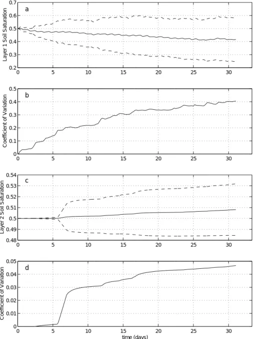
Figure 1 shows the results from the forcing realisations using method 1. In Fig. 1a and 1c, the mean soil moisture evolution in layers 1 and 2 is plotted over the month while the corresponding error propagation for each layer is shown in Fig. 1b and 1d. The variability in output caused by the

unique temporal structure of each precipitation time series can be seen clearly. For the error, the coefficient of variation is zero at the beginning of the month where the initial condition is specified. As different precipitation time series are routed through the model, the differences in temporal structure show up in the soil moisture response, causing the error to increase with time. For layer 1, which responds relatively quickly to the precipitation forcing, the error grows most quickly during the first five days and then begins to level off slowly, reaching a standard error of ~ 40% of the mean by the end of the month. For layer 2 which responds

0 5 10 15 20 25 30 0.2 0.3 0.4 0.5 0.6 0.7

Layer 1 Soil Saturation

a 0 5 10 15 20 25 30 0 0.1 0.2 0.3 0.4 0.5 Coefficient of Variation b 0 5 10 15 20 25 30 0.48 0.49 0.5 0.51 0.52 0.53 0.54

Layer 2 Soil Saturation

c 0 5 10 15 20 25 30 0 0.01 0.02 0.03 0.04 0.05 Coefficient of Variation d time (days)

Fig. 1. Results using method 1 disaggregation scheme in the VIC-2L model. a) Mean soil

saturation for layer 1 (dashed lines represent ± one standard deviation); b) Coefficient of variation in layer 1 soil moisture; c) Mean soil saturation for layer 2 (dashed lines represent

only indirectly, and thus more slowly, to precipitation events (through drainage from layer 1) the error is relatively small over the first few days, with a relatively large increase by day 6 before levelling off to a value of ~5% of the mean. This error is much smaller due to the fact that layer 2 does not respond directly to precipitation events.

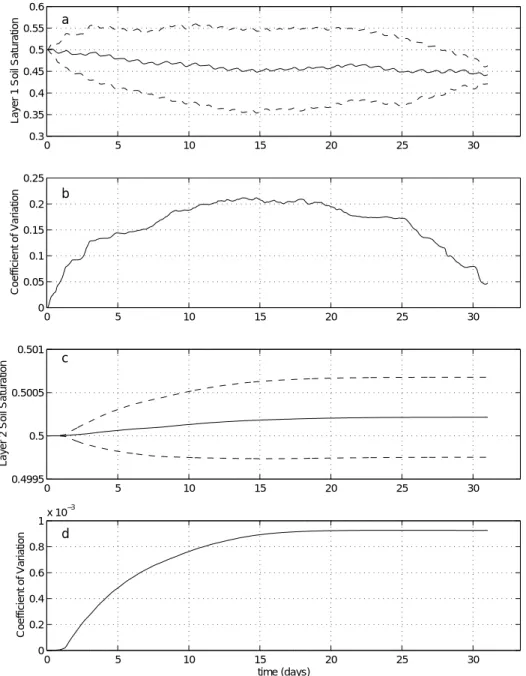
Figure 2 shows the same results as in Fig. 1, but for precipitation forcing disaggregated using method 2. The primary difference in model forcing lies in the added constraint imposed in method 2, where precipitation realisations are sampled only when they are within a

prescribed tolerance of the known monthly total rainfall. For method 2, 100 precipitation realisations were again routed through the model; however, for each realisation the monthly accumulation of precipitation is within 5 mm of the known monthly total used in the disaggregation technique. The effect of this closure leaves a clear imprint on the model output. For layer 1, the error is again zero at the beginning of the month. It increases to a maximum value (20% of the mean) during the month but, instead of remaining relatively constant at this value, it decreases to a terminal value of less than 5% of the mean at the end of the month. The reason for this

Fig. 2. Results using method 2 disaggregation scheme in the VIC-2L model. a) Mean soil saturation for

layer 1 (dashed lines represent ± one standard deviation); b) Coefficient of variation in layer 1 soil moisture; c) Mean soil saturation for layer 2 (dashed lines represent ± one standard deviation);

d) Coefficient of variation in layer 2 soil moisture

0 5 10 15 20 25 30 0.3 0.35 0.4 0.45 0.5 0.55 0.6

Layer 1 Soil Saturation

a 0 5 10 15 20 25 30 0 0.05 0.1 0.15 0.2 0.25 Coefficient of Variation b 0 5 10 15 20 25 30 0.4995 0.5 0.5005 0.501

Layer 2 Soil Saturation

c 0 5 10 15 20 25 30 0 0.2 0.4 0.6 0.8 1x 10 −3 Coefficient of Variation d time (days)

markedly different behaviour is that each realisation conserves the total amount of precipitation over the month, which serves as a weak constraint that bounds the error in the partitioning of the precipitation input over the month. Based on method 2, the maximum error within the month for layer 1 is reduced by a factor of 2 and the error at the end of the month is reduced by a factor of 5. These errors are important for hydrological studies over several months where it would be desirable to account for the month-to-month errors. For layer 2, the error does not reach a maximum and then decrease as for layer 1 due to the slower response time. However, the error is reduced by a factor of 50 when compared to results from method 1. The results shown here are representative of results obtained for several other cases covering different seasons and levels of precipitation forcing in Margulis and Entekhabi (1998). Overall, the results show that method 2 reduces significantly the amount of error propagated through the land surface model.

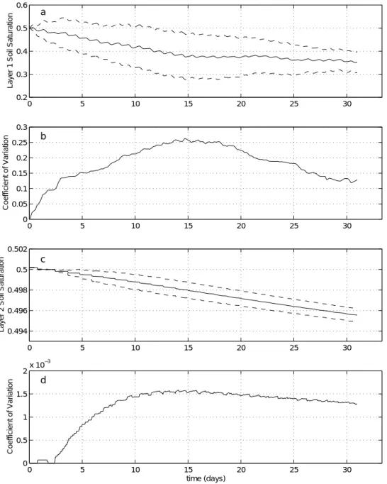
To make sure these results were not model dependent, method 2 realisations were also routed through a more detailed high-resolution soil water transport model (Vogel

et al., 1996). The model is sensitive to rainfall rate and

includes ponding, an additional nonlinear process that should introduce additional errors. For the high-resolution model, the same forcing, soil parameters and lower boundary condition were used and the soil moisture was averaged over the nodes corresponding to layers 1 and 2 in the VIC-2L model (the high-resolution model has 150 layers ranging from 1 cm to 10 cm in thickness). The results in Figs. 1 and 2 are shown in Fig. 3 for the high-resolution model. The maximum error and end-of-month errors for both layers 1 and 2 are slightly larger than those shown in Fig. 2, which is most likely due to the additional non-linearities discussed above. However, qualitatively the results are similar and show that the realisations generated using method 2 are superior to those from method 1 regardless of the model used.

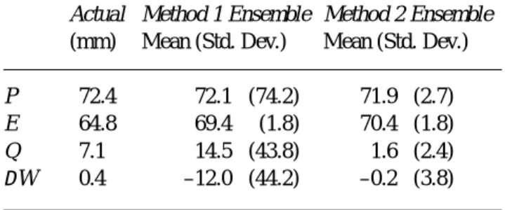
Finally, it is of interest to see how well the integrated water balance components are reproduced over the month by the disaggregation schemes. Table 2 shows the integrated precipitation (P), evapotranspiration (E), runoff (Q) and change in storage (DW) for the VIC-2L simulations using

the actual precipitation time series (which was aggregated and used as input to the disaggregation schemes), and the realisations from methods 1 and 2. Table 2 again shows that the total monthly precipitation is preserved on average in the realisations generated using both methods. The primary benefit of method 2, however, is that the standard deviation about this mean is very small compared to method 1. Therefore, the differences in the water balance components derived from the actual precipitation time series and method 2 realisations are due solely to the temporal structure of the

Table 2. Comparison of integrated monthly water balance

components resulting from actual precipitation forcing and from realisations generated using methods 1 and 2

Actual Method 1 Ensemble Method 2 Ensemble

(mm) Mean (Std. Dev.) Mean (Std. Dev.)

P 72.4 72.1 (74.2) 71.9 (2.7)

E 64.8 69.4 (1.8) 70.4 (1.8)

Q 7.1 14.5 (43.8) 1.6 (2.4)

DW 0.4 –12.0 (44.2) –0.2 (3.8)

precipitation forcing, whereas for method 1, differences exist due to a combination of differing total precipitation as well as temporal structure. For both methods 1 and 2, the average evapotranspiration is slightly overestimated. This is due primarily to the fact that for both methods the average dry time (as represented by the probability of no rain), in which evapotranspiration is high, is overestimated compared to the actual time series (see Table 1). For method 2, where P is conserved for every realisation, the overestimation in E leads to an underestimation of the other water balance components (Q and DW). For method 1, the high variability in P actually

causes an overestimation of runoff and a larger change in storage. These results show the superiority of method 2 over method 1 in that it reproduces the surface water balance more accurately.

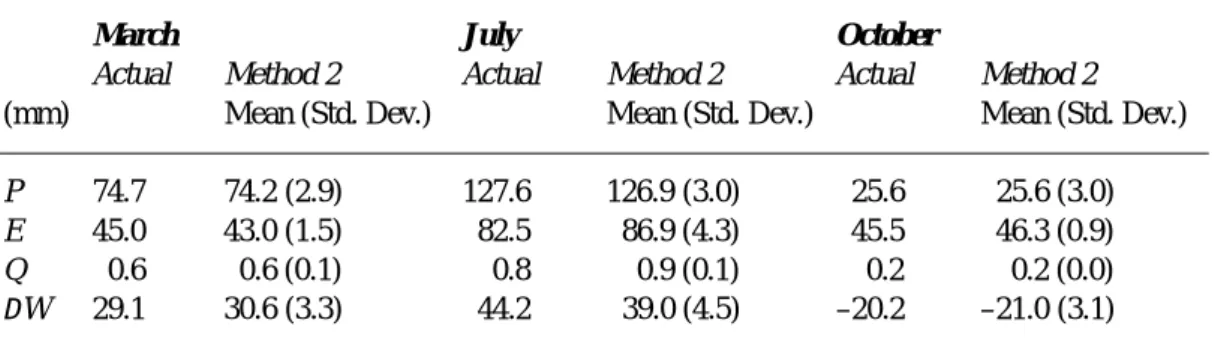
To test the robustness of method 2, other runs, for different seasons and different soil moisture conditions were performed. Tables 3 and 4 show results for a “moderate” March (75 mm of rainfall), “high” July (128 mm), and “low” October (26 mm) precipitation case (each case had a medium soil moisture initial condition). The actual partitioning of the precipitation between evapotranspiration, runoff and change in soil moisture is compared to that predicted by method 2. Overall, method 2 reproduces the surface water balance quite well. There appears to be no systematic bias in any of the water balance components. For the high precipitation case (July), evapotranspiration and runoff are slightly overestimated, which is balanced by a slight underestimation in the change in soil moisture. For the low precipitation case (October), runoff is reproduced exactly, so that the slight overestimation in evapotranspiration is balanced by an underestimation in change in soil moisture. Note however that some of these differences are due to the fact that total precipitation forcing is not reproduced exactly, but instead within a tolerance which leads to slight differences in the total amount of water forcing the land surface.

Another set of tests forced the land surface with the same precipitation amount, but with a “wet” (95% saturation),

Fig. 3. Results using method 2 disaggregation scheme in the high-resolution model. a) Mean soil

saturation for layer 1 (dashed lines represent ± one standard deviation); b) Coefficient of variation in layer 1 soil moisture; c) Mean soil saturation for layer 2 (dashed lines represent ± one standard

deviation); d) Coefficient of variation in layer 2 soil moisture

0 5 10 15 20 25 30 0.2 0.3 0.4 0.5 0.6

Layer 1 Soil Saturation

a 0 5 10 15 20 25 30 0 0.05 0.1 0.15 0.2 0.25 0.3 Coefficient of Variation b 0 5 10 15 20 25 30 0.494 0.496 0.498 0.5 0.502

Layer 2 Soil Saturation

c 0 5 10 15 20 25 30 0 0.5 1 1.5 2x 10 −3 Coefficient of Variation d time (days)

“moderate” (50% saturation), and “dry” (10% saturation) soil moisture initial condition. Method 2 for the moderate and dry cases again reproduces the water balance quite well. The largest errors occur in runoff for the wet case. This is a result of a runoff threshold processes in VIC-2L, for which there is a large change in runoff at a specified high soil moisture threshold. This strong non-linearity causes a significant difference between the actual runoff and that predicted on average by method 2. However, the error occurs only at the very high (95%) saturation levels used in this

case. Over most of the range of soil moisture conditions, the error is much less severe and method 2 is able to reproduce the surface water balance accurately.

Conclusions

In this study, two techniques were proposed for the temporal disaggregation of monthly precipitation estimates that are obtained from satellites. Due to the non-linearities involved in the partitioning of precipitation at the land surface, these

techniques are needed to make the coarse temporal estimates useful for large scale hydrological studies. Both techniques have the desirable property that the known total monthly precipitation is preserved on average at all levels of aggregation. Method 2 improves greatly on method 1 by conserving the total monthly precipitation in every realisation (within a prescribed tolerance). This has a direct impact on the error propagation in the partitioning of precipitation at the land surface. By routing an ensemble of precipitation realisations through a land surface model, the error introduced by using the disaggregated precipitation time series was characterized. For the VIC-2L land surface model, the error introduced by method 1 reaches a level of approximately 40% of the mean soil moisture during the course of a month in the layer that responds directly to precipitation forcing. For method 2, the added constraint that each realisation conserves the accumulated precipitation over the month acts as a weak constraint on the water balance over the course of the month, which significantly reduces the error in the partitioning of the precipitation input to less than 5% of the mean. When compared to a detailed high-resolution model of the unsaturated zone (which was sensitive

to rain rate and ponding) the results using method 2 are very similar, indicating that the error propagation is similar across models. In examining the integrated monthly water balance components, similar gains in reducing the error were shown for method 2, which was relatively robust in its ability to reproduce the surface water balance for different seasons (with differing precipitation inputs) and for different soil moisture initial conditions. Overall, these results show that disaggregated precipitation forcing obtained from method 2 can be used in large scale water balance studies without introducing significant error.

Acknowledgments

This work was supported by the National Aeronautics and Space Administration Grants NAGW-4164 and NAGW 4766.

References

Adler, R., Negri, A., Keehn, P. and Hakkarinen, I. M., 1992. Estimation of monthly rainfall over Japan and surrounding waters from a combination of low-orbit microwave and geosynchronous

Table 3. Comparison of integrated monthly water balance components resulting from actual precipitation

forcing and from realisations generated using method 2 for: March (moderate rainfall), July (high rainfall), and October (low rainfall) simulations

March July October

Actual Method 2 Actual Method 2 Actual Method 2

(mm) Mean (Std. Dev.) Mean (Std. Dev.) Mean (Std. Dev.)

P 74.7 74.2 (2.9) 127.6 126.9 (3.0) 25.6 25.6 (3.0)

E 45.0 43.0 (1.5) 82.5 86.9 (4.3) 45.5 46.3 (0.9)

Q 0.6 0.6 (0.1) 0.8 0.9 (0.1) 0.2 0.2 (0.0)

DW 29.1 30.6 (3.3) 44.2 39.0 (4.5) –20.2 –21.0 (3.1)

Table 4. Comparison of integrated monthly water balance components resulting from actual precipitation

forcing and from realisations generated using method 2 with: wet, moderate, and dry soil moisture initial conditions

Wet Moderate Dry

Actual Method 2 Actual Method 2 Actual Method 2

(mm) Mean (Std. Dev.) Mean (Std. Dev.) Mean (Std. Dev.)

P 74.7 74.2 (2.9) 74.7 74.2 (2.9) 74.7 74.2 (2.9)

E 45.0 43.0 (1.5) 45.0 43.0 (1.5) 19.5 21.0 (6.1)

Q 9.4 17.6 (11.0) 0.6 0.9 (0.1) 0.2 0.2 (0.0)

IR data. J. Appl. Meteorol., 18, 335–356.

Bo, Z., Islam, S. and Eltahir, E.A.B., 1994. Aggregation-disaggregation properties of a stochastic rainfall model. Water

Resour. Res., 30, 3423–3435.

Collins, C., 1989. Application of weather radar systems: A guide

to uses of radar data in meteorology and hydrology. Halsted Press,

New York.

Entekhabi, D., Rodriguez-Iturbe, I. and Eagleson, P., 1989. Probabilistic representation of the temporal rainfall process by a modified Neyman-Scott rectangular pulses model: Parameter estimation and validation. Water Resour. Res., 25, 295–302. Groisman, P.Y. and Legates, D., 1994. The accuracy of United States

precipitation data. Bull. Amer. Meteorol. Soc., 75, 215–227. Hawk, K.L. and Eagleson, P., 1992. Climatology of station storm

rainfall in the continental U.S.: Parameters of the Bartlett-Lewis and Poisson Rectangular Pulses models. Technical Report 336, Massachusetts Institute of Technology, Department of Civil Engineering.

Hershenhorn, J. and Woolhiser, D.A., 1987. Disaggregation of daily rainfall. J. Hydrol., 95, 299–322.

Huffman, G.J., Adler, R.F., Arkin, P., Chang, A., Ferraro, R., Gruber, A., Janowiak, J., McNab, A., Rudolf, B. and Schneider U., 1997. The global precipitation climatology project (GPCP) combined precipitation dataset. Bull. Amer. Meteorol. Soc., 78, 5–20. Liang, X., Lettenmaier, D., Wood, E. and Burges, S., 1994. A simple

hydrologically based model of land surface water and energy fluxes for general circulation models. J. Geophys. Res., 99, 14,415–14,428.

Marani, M., Grossi, G., Wallace, M., Napolitano, F. and Entekhabi, D., 1997. Forcing, intermittency, and land surface hydrological partitioning. Water Resour. Res., 33, 167–175.

Margulis, S.A. and Entekhabi, D., 1998. Temporal disaggregation of satellite derived monthly precipitation estimates for use in hydrological applications. Technical Report 344, Massachusetts Institute of Technology, Department of Civil Engineering. Rodriguez-Iturbe, I., Gupta, V.K. and Waymire, E., 1984. Scale

considerations in the modelling of temporal rainfall. Water Resour.

Res., 20, 1611–1619.

Salvucci, G. and Song, C., 2000. Derived distributions of storm depth and frequency conditioned on monthly total precipitation: Adding value to historical and satellite-derived estimates of monthly precipitation. J. Hydrometeorol., 1, 113–120. Valdes, J. B. and Rodriguez-Iturbe, I., 1985. Approximations of

temporal rainfall from a multidimensional model. Water Resour.

Res., 21, 1259–1270.

Vogel, T., Huang, K., Zhang, R. and van Genuchten, M.T., 1996. The HYDRUS code for simulating one-dimensional water flow, solute transport, and heat movement in a variably-saturated media (Version 5.0). Technical Report 140, U.S.D.A., Salinity Laboratory, Agricultural Research Service.

Wilks, D. S., 1989. Conditioning Stochastic Daily Precipitation Models on Total Monthly Precipitation. Water Resour. Res., 25, 1429–1439.