Dynamic inventory management with expediting

Dynamic Inventory Management with Expediting

by

Chiwon Kim

B.S., Mechanical and Aerospace Engineering,

Seoul National University (2002)

M.S., Mechanical Engineering,

Massachusetts Institute of Technology (2004)

Submitted to the Department of Mechanical Engineering

in partial fulfillment of the requirements for the degree of

Doctor of Philosophy in Mechanical Engineering

at the

MASSACHUSETTS INSTITUTE OF TECHNOLOGY

June 2008

@

Massachusetts Institute of Technology 2008. All rights reserved.

A u th o r ...

...

...

Department of Mechanical Engineering

March 31, 2008

Certified by...

Professor, Department of

Certified by...

David Simchi-Levi

Civil and Environmental Engineering and the Engineering

Q 4- Di I II

Thpsis Supervisor

---S

ay Sarma

Professor, Department of Mechanical Engineering

Thesis Supervisor

Accepted by...- ... : ....

Lallit

irman, Department Committee on Graduate Students

MASSACH.SETS INS E Cha

OF TECHNOLOGY

JUL

2

9 2008

LIBRARIES

MCH

Dynamic Inventory Management with Expediting

Chiwon Kim

Submitted to the Department of Mechanical Engineering on March 31, 2008, in partial fulfillment of the

requirements for the degree of

Doctor of Philosophy in Mechanical Engineering

Abstract

In modern global supply chains, goods travel stochastically from suppliers to their final des-tinations through several intermediate installations such as ports and distribution facilities. In such an environment, the supply chain must be agile to respond quickly to demand spikes. One way to achieve this objective is by expediting outstanding orders from the intermediate installations through premium delivery. In this research, we study the optimal expediting and regular ordering policies of a serial supply chain with a radio frequency identification deployment at each installation. Radio frequency identification technology allows capturing the state of the system, i.e., the time and location of goods, at any point in time, and thus enables to expedite outstanding orders directly to the destination, which faces stochastic demand.

We identify systems, called sequential, that yield simple and tractable optimal policies. For sequential systems, outstanding orders including expediting do not cross in time. For such systems, we find that the optimal policies of expediting and regular ordering are the base stock type policies. The directional sensitivity of the base stock levels with respect to expediting costs is also obtained. We provide an important managerial insight on the radio frequency identification technology: we need to actively use the additional information from the radio frequency identification technology through new business processes such as expediting to unveil more benefits from the supply chain. On the other hand, orders may cross in time for systems that are not sequential, thus in such a case optimal policies are hard to obtain. We propose a heuristic for such systems and discuss its performance and limitation. Lastly, as an extension to the model, we study the optimal policies of expediting and regular ordering when there is an expiry date on outstanding orders. The optimal expediting policy identifies a number of base stock levels depending on the age of the orders, but the structure of the optimal policy remains simple for sequential systems.

Thesis Supervisor: David Simchi-Levi

Title: Professor, Department of Civil and Environmental Engineering and the Engineering Systems Division

Thesis Supervisor: Sanjay Sarma

Acknowledgments

First and foremost, I would like to thank my advisor Professor David Simchi-Levi for his valuable guidance throughout my PhD years. He is not only an excellent scholar with deep insights, but also a great advisor on both research and life. I indeed appreciate his wisdom at every key point of my research. I was very fortunate to become his student even though he is famous for being very selective in choosing his students and my home department is rather far from the field of supply chain management. It has truly been an honor and a pleasure to work with him.

Next, I would like to thank my co-advisor Professor Diego Klabjan at Northwestern University. It is difficult to fully acknowledge here the extent of his support and express my gratitude. He is simply an amazing researcher, teacher, and mentor in every aspect of life. I can discuss anything with him, and he has been always there to help me and to encourage me. He was at MIT during 2005-2006 for his sabbatical year, and that is how I started working with him. Even after he left for Northwestern University, he remained as my co-advisor and guided me through every step of my research. Without him, I could not have completed my research.

I would like to thank my thesis committee members, Professors Sanjay Sarma and Jeremie Gallien. Professor Sarma has been a good supporter of my research and always encourages me to keep going forward. Professor Gallien provided insightful comments and suggestions on this research. I appreciate all of their input and time. Also, I am very grateful to my Master's thesis advisor, Dr. Stanley Gershwin. He has always been a great advisor and mentor. I am greatly indebted to him for his help during my early days at MIT.

I would like to thank all of my friends at MIT for making my life really enjoyable: Sunghwan Jung, Youngjae Jang, Hyuksang Kwon, Jaemyung Ahn, Sangwon Byun, and Sang-Il Lee, among others. I cannot name them all here since they are so many. I am equally grateful to every one of them, and my life would never have been the same without them. Finally, I am indebted to my family for their support. My parents and my sister are always supportive for my studies far away from home. My wife, Dooran Kim, gives me endless support, encouragement and love during ups and downs. This thesis could not have been finished without her support.

Contents

1 Introduction 8

1.1 Motivation ... ... . 8

1.2 Stochastic Inventory Theory: Review ... . . . . . . . . ... . 11

1.3 Road Map ... ... . ... 15

2 Deterministic Lead Time Model 17 2.1 Introduction ... ... ... 17

2.2 Model Statement .. ... .. 20

2.3 Sequential Systems .. ... . 22

2.4 Optimal Policies for Sequential Systems ... . . . . . . . . . ... . 25

2.5 Additional Results .. ... . 34

3 Stochastic Lead Time Model 36 3.1 Introduction ... ... . ... 36

3.2 Model Statement .. ... 40

3.3 Sequential Systems .. ... . 44

3.4 Optimal Policies for Sequential Systems ... . . . . . . . . ..... 49

3.4.1 Preliminaries .. ... . 49

3.4.2 Optimal Policies . ... . 51

3.5 Results on the Expediting Base Stock Levels of Sequential Systems . . . . . 57

4 Non-Sequential Systems 60 4.1 Introduction ... ... . 60

4.2 The Extended Heuristic for Nonsequential Systems . . . ... .. 61

5 Raw Materials with an Expiry Date

5.1 Introduction ... ... 5.2 Model Statement ...

5.3 Sequential Systems . . . . 5.4 Optimal Policies for Sequential Systems .

5.4.1 Preliminaries ...

5.4.2 Optimal Policies . . . . 5.4.3 Illustration of the Optimal Policy.

6 Conclusion

A Proofs and Additional Lemmas

71 . . . . . 71 . . . . . 73 . . . . . 74 . . . . . 76 . . . . . 76 . . . . . 80 . . . . . 87

List of Figures

1-1 Possible scenarios of uncertainties . ... . 9

1-2 An illustration with a two-installation supplier and manufacturing facilities 10 2-1 The underlying inventory system . ... . 20

2-2 Expediting a partial order from installation i ... . . . . . . . . .... .. . 22

2-3 An illustration of the optimal policies ... . . . . . . . . ... . 32

2-4 The Base Stock Levels with Nonstationary Demand . . . . 33

3-1 A regular movement driven by a realized w of W . . . .... .. 42

3-2 The next state transition . ... . 43

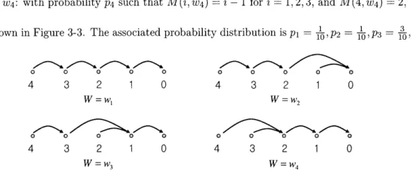
3-3 The movement patterns . ... . 49

3-4 The movement patterns . ... . 51

3-5 Directional sensitivity of base stock levels .... . . . . . . . . ..... 58

4-1 Improvements in cost-to-go of the derivative method with respect to the extended heuristic .. ... . 64

4-2 Local optimality and limitation of the extended heuristic . . . . 64

4-3 Simulation results .. ... . 69

4-4 The base stock levels .. ... . 70

5-1 Sequence of events .. ... . 73

5-2 Physical installations with age bins . ... . 74

5-3 Stage inventory level and location representation .. . . . . . . . . ..... . 74

5-4 Monotonicity across installations of the same age . . . . . . . . . ..... . 87

5-5 Monotonicity within an installation . ... . 88

5-7 Monotonicity of nonempty age bins in all installations . . . . 89 5-8 The simple structure of the optimal expediting policy . . . . 89

Chapter 1

Introduction

1.1

Motivation

Recent globalization has brought increased complexity in supply chains. With facilities in supply chains spread throughout the globe, lead times are growing and becoming more volatile. Fierce competition among global supply chains is observed. According to Lee (2004), an important challenge for competitive advantage is to build agile, adaptable, and

aligned supply chains. Agility, adaptability, and alignment of supply chains mean the

fol-lowing:

* Agility: ability to respond quickly to short-term changes in demand or supply

* Adaptability: ability to adjust supply chain design to accommodate medium or long-term market changes

* Alignment: ability to establish incentives for supply chain partners to improve per-formance of the entire chain

Among these, our focus is mainly on the issue of improving the agility of today's supply chains. Agility can be improved by promoting the flow of information between suppliers and customers and developing collaborative relationships with suppliers. For instance, if suppliers provide more information on shipments along with more delivery options for different rates, then the agility of supply chains can be improved. In this research, we try to improve the agility of a supply chain through expediting outstanding orders based on extra information about goods in transit from the supplier. Rather than just waiting for regular

orders to be delivered, a firm may expedite partial or complete orders in transit through premium delivery, such as by air, with extra cost, to improve agility.

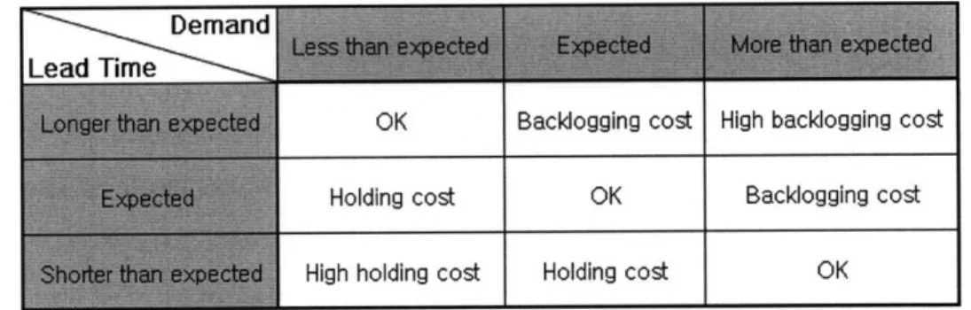
To see potential benefits, let us consider an inventory system that faces stochastic lead time and demand. Usually, the optimal operation of an inventory system can be achieved through balancing holding and backlogging costs under certain expectations on lead time and demand. If the realized demand is higher than expected, a backlogging cost is incurred. On the other hand, if the demand is lower than expected, a holding cost occurs. The same case happens with stochastic lead time: if the lead time is shorter than expected, a backlogging cost is incurred, and otherwise, a holding cost occurs. Figure 1-1 summarizes 9 possible scenarios due to these uncertainties. Improved agility through expediting can

Backlogging cost High backlogging cost Holding cost OK Backlogging cost High holding cost Holding cost OK

Figure 1-1: Possible scenarios of uncertainties

directly reduce the backlogging cost due either to high demand, short lead time, or both. If demand spikes, we may expedite outstanding orders to meet the excessive demand to reduce the undesirable backlogging cost. Also, we may shorten the undesirably prolonged lead time of certain orders through expediting. Not only the backlogging cost, but also the holding cost, can be reduced by improved agility through expediting, since the supply chain with expediting does not require as much safety stock as the one without expediting options. Reduced safety stock generally lowers the holding cost. Therefore, the improved agility through expediting certainly reduces unexpected costs, both holding and backlogging costs of the supply chain.

However, the practice of expediting incurs expediting costs. Therefore, in order to minimize the total supply chain costs, which include the expediting costs, one has to know how to use the expediting options wisely. In this research, we study how to optimally exploit expediting to increase agility, which is our central focus. More specifically, we address the

questions of what the optimal expediting policy is, whether the policy is practical, and what the corresponding optimal regular ordering policy is. Additionally, we discuss the questions of what the effects of expediting costs on the optimal policy are, what information systems we need to support expediting, and how we can extend the model to accommodate more real-world situations. We answer all these questions in the following chapters.

Simple but Nontrivial Illustration1

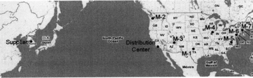
Suppose that a company in South Korea makes a high-value product such as LCD panels. As the leading supplier, it supplies its panels to multiple TV and computer monitor man-ufacturers spread throughout the US. It operates a distribution center in Long Beach, CA, for operational efficiency. Because of the weight and volume of LCD panels, it usually uses ocean shipping rather than air to transport LCD panels to the distribution center, and then it uses ground transportation to each of the manufacturers. The lead time is stochastic, between 2 and 6 weeks. While there are several manufacturers, our focus is on the manu-facturer labeled M-1. To increase agility, M-1 utilizes expediting. M-1 may expedite LCD panels from the supplier in South Korea by air to M-1, or from the distribution center in Long Beach by air to M-1. See Figure 1-2.

Figure 1-2: An illustration with a two-installation supplier and manufacturing facilities

In this thesis, we discuss more general models than the one just illustrated. However, it is important to remark that, even though it looks simple, this illustration contains all the complex features of much more general models, which may have multiple installations spread all over the world.

1.2

Stochastic Inventory Theory: Review

In this section, we give a brief review of stochastic inventory theory. For a broader review, we refer to Simchi-Levi et al. (2004) and Porteus (2002).

Basic inventory model

As the simplest multi-period case, consider a periodic-review, single-item inventory problem. The planning horizon is T time periods. This inventory faces stochastic demand, and the demand distribution is known and independent for each time period. There is a single supplier of the inventory with the procurement cost of c per unit, and the order lead time is instantaneous compared with the time period. Excessive demand is backlogged at cost

b per unit per time period and fulfilled in the following time periods. On the other hand,

excessive inventory incurs the holding cost of h per unit per time period.

Let us denote the demand by D and the inventory on hand by v. The inventory manager places an order of amount u at the beginning of a time period, which is the decision variable for that time period. At time period T + 1, the inventory on hand can be returned to the supplier at the per unit cost of c. For simplicity, we do not discount future costs, and do not consider any fixed ordering costs. For convenience, let us define L(x) = E[b. (x- D)- + h -(x - D)+], where (x)+ = max{x, 0} and (x)- = min{x, 0}.

Let us denote by Jt(v) the cost-to-go at time period t with on-hand inventory v. The dynamic programming optimality equation reads

Jt(v) = min{cu + L(u + v) + E[Jt+i (u + v - D)]}, u>0

where JT+l (v) = -cv. It is common to introduce y = u + v. Then we have

Jt(v) = min{cy + L(y) + E[Jt+l (y y>v - D)]} - cv,

where JT+I (v) = -cv. Let us first examine JT(v). We have

JT(v) = min{cy + L(y) + E[-cy + cD]} - cv = min{L(y)} + c(E[D] - v).

can find a quantity y* that minimizes L(y), or yý = argmin{L(y)}. The optimal ordering policy at time period T is to order y - v if v _ yý, and otherwise order nothing. This policy

is called the base stock policy, and yý is the base stock level of time period T with respect to

v. Cost-to-go Jt(v) has a special structure. It is the sum of L(yý) - cv and a monotonically nondecreasing convex function g(v), where g(v) = 0 for v < yý and g(v) = L(v) - L(yý) for v > yý.

Now, assume J+l (v) is convex for a fixed t such that t +1 T. By the same reasoning, cy + L(y)

+

the minimizer by yt*, or yt = argminy{cy + L(y) + E[Jt+i(y - D)]}. Then the optimal

policy is again the base stock policy with the base stock level yt. Finally, Jt(v) is again a convex function under the base stock policy. By the inductive argument, we conclude that the base stock policy with the base stock level yt for time period t is optimal for this inventory problem.

Finite lead time inventory model

In certain cases, lead time cannot be considered instantaneous compared to the review pe-riod. In such cases, we consider an inventory with a finite lead time of multiple time periods. Lead time can be either deterministic or stochastic, and here we review the deterministic lead time case. Since the lead time is longer than a review period, we have to keep track of multiple order amounts that are placed within the lead time. Let us denote by v0 the

on-hand inventory and by vi the outstanding order amount that has i time periods remaining until delivery. Let L be the lead time. Then the state variables are (vo, v, ... , VL-1). The optimality equation reads

Jt(vo, v1, ,VL-1) = min{cu

+

+

+

vi

u>O

where JT+l (vo, vi, .. . , VL-1) = -c(vo

+

+ VL-1.

+ VL-1

Multi-echelon inventory model

The multi-echelon inventory problem is introduced in Clark and Scarf (1960). It has a series of installations, where an installation supplies the next one, and exogenous demand is realized at one end of the chain. Let us denote by Ij the jth installation, 0 < j < K,

where 10 faces exogenous demand, IK has infinite amount of inventory, and Ij places orders to Ij+l. The lead time between two consecutive installations can be either zero or finite time periods. Let the lead time be L time periods.

The notion of an echelon is important. An echelon is a certain subsystem of the entire supply chain. More specifically, by echelon i we mean the subsystem from I0 to Ii. Therefore, echelon 0 is just I0, echelon L is the whole system, and thus there are a total of L+1 echelons. Echelon stock is the sum of all stock in the corresponding echelon plus outstanding orders that are supposed to be delivered within L time periods to the echelon. Let us denote the echelon-i stock by xi.Inventory position, which is defined above, is simply echelon-(L - 1) stock.

The optimal policy of a multi-echelon inventory system is the base stock policy adapted to the multi-echelon setting. Consider echelon i. Echelon i receives stock from Ii+1 up to the availability in Ii+l. The optimal policy for ordering from Ii+1 for echelon i is the base stock policy with respect to echelon-i stock x', but the ordering amount is limited by the current inventory level at Ii+l. From echelon 0 to echelon L - 1, orders are made based on the base stock policies, with different base stock levels for each echelon at each time period.

Finite shelf life inventory model

Nahmias (1975) and Fries (1975) studied a periodic review, zero lead time inventory problem with deterministic shelf life. Here we briefly introduce the approach of Nahmias (1975). Let us denote by xi the amount of product on hand that will perish exactly i periods into the future. The state of the system can be represented as x = (Xm-1, Xm-2,"" ,X ₁). For

con-venience, let us define x(i) = (xi, x_,- ,xi), i.e., x(m - 1) = x, and wi = Ej= xj. The inventory position is x = wm-1. Demand density

f

* si[y,x,D] = (xi+l - (D - wi)+)+ for 1 < i < m- 2,

* Sm-1[y,x,D] = y - (t - Wm-l)+ (backlogging).

Demand Aj,n [x(j)] over

j

j - 1 that cannot be met by allocations of supply, which would have been outdated by the beginning of period n +

j.

* Aj,n[x(1)] = (Dn - Xl) + ,

* A2,n[x(2)] = (Dn+1 + (Dn - x1)+ - x2)+ = (Dn+l1 + AI,n•[(1)]- X22)+

* Am-i,n[x(m - 1)] = (Dn+m-2 + Am-2,n[x(m - 2)] - Xm-l)+.

Quantity y- Am-l,n[x(m- 1)] is the total amount of the fresh order on hand at the start of period m + n - 1. The amount of the fresh order that perishes is R*,n = (y

-Dm+n-1- Am-,n[x(m-1)])+. To get the distribution of Rm,n, Nahmias (1975) first defines Gj, [x(j)] = Prob(Dj+n_ + Aj-l,n(x(j - 1)) _ xj), which is the probability that there will be outdating at the end of period n +

j

Gy,n[x(j)] = Gj-l,n[v + Xj-1, x(j - 2)]f(xj - v)dv,

where Gi(t) = F(xi). From the definition of Gm,n, it follows that Prob[R*,n 5 t] =

1 - Gm,n(y - t,x), for t > 0 and Prob[R*,,n < t] = 0 for t < 0. Since demand is a nonnegative random variable, E[R*,n] = f~' Gm,n(t, x)dt. The single period cost Ln(x, y) is

given by

fX+Y 00 Y

Ln(x, y) = cy + h (x + y - t)f(t)dt + r (t - x - y)f(t)dt + 0 Gm,n(t, x)dt.

O x+y0

It can be shown that Ln(x, y) is convex in y for a fixed x. Let Cn(x) be the minimum expected discounted cost when there are n remaining periods. Similarly, let Ln(x, y) be the cost when there are n remaining periods. We also define

There is a functional relation of Cn(x) = infyŽoBn(x,y). Let us define t - F-l [r " Under some mild assumptions, the following holds.

* Bn (x, y) is convex in y for all x.

* If x < , then there exists a unique solution of the following equation:

8Bn(x, y)

_OB

_(X,

y=yn(x)

* The optimal policy is to order Yn(x) if X < .

* Denote by y(i) differentiating with respect to i-th argument. Then -1 < yh)(x) <

y(x) y)(x) <- < yn m-1)(x) _{< 0. This means that if the initial stock of}

inven-tory at any age level is increased by one unit, the optimal order quantity decreases, but by less than a single unit. Furthermore, the optimal order quantity is more sensitive with respect to the newer inventory.

* If demand is backlogged, then yn(x) = yn(O) + IXm-1

.

Nahmias (1982) states that the actual computation is impractical if m > 3.

1.3 Road Map

This thesis consists of four main topics, each of which is introduced independently in the respective chapters. Since the problem of finding an optimal expediting policy is quite demanding, in Chapter 2 we first restrict our attention to the problem with a deterministic lead time. Even though the lead time is deterministic, finding an optimal policy is still challenging, and it requires a careful treatment. The concept of sequential systems appears first in this chapter.

In Chapter 3, we extend the model so that the lead time is stochastic. With stochastic lead time, we have to capture the locations of outstanding orders in order to expedite them. Radio Frequency Identification (RFID) is introduced for this purpose in this chapter. Also, the concept of sequential systems is generalized to accommodate stochastic lead time. The optimal policies are simple and elegant. The solution methodology is complex, but manageable for sequential systems.

In Chapter 4, we consider systems that are not sequential, and perform a numerical study on non-sequential systems with a proposed heuristic policy. The heuristic policy is quite robust for the systems that are close to being sequential. We discuss its performance and limitations.

Chapter 5 extends the model of Chapter 3 so that orders in transit can have a certain expiry date until delivery, which is the most general model treated in the thesis. The optimal policy for sequential systems identifies a number of parameters, but the structure of the optimal policy remains simple.

We conclude in Chapter 6 with a detailed discussion of contributions made in this thesis and directions for further research.

Chapter 2

Deterministic Lead Time Model

2.1

Introduction

We consider a supply chain that consists of a supplier and a manufacturing facility. Between them, there are multiple intermediate installations such as ports and distribution centers. The manufacturer faces stochastic demand, periodically reviews inventory on hand, and places orders at the supplier. In regular delivery, orders pass through all installations with a deterministic lead time. In addition to regular delivery, expedited delivery is available with extra cost for all or part of the outstanding orders in the pipeline. The manufacturer may expedite orders based on the current inventory status and the demand forecast. When expedited, orders instantly arrive at the manufacturing facility and they are ready to fulfill upcoming demand. In our setting, all decisions are made by the manufacturer, and it is assumed that the manufacturer cannot influence inventory among installations other than into the manufacturing facility. As a consequence, expediting from any installation is allowed only when the destination is the manufacturing facility. This is reasonable when the manufacturing facility is an independent company from the remaining installations and thus cannot instantiate expediting between two other installations. Without expediting, it is well known that the optimal regular ordering follows the base stock policy with respect to the inventory position.

In general, the problem of finding an optimal inventory control policy with respect to regular ordering and expediting is difficult, and it depends critically on the system parameters such as the expediting costs. We introduce the notion of sequential systems, where it is never optimal to expedite from an installation before expediting all outstanding

orders in the downstream installations. The optimal regular and expedited orders preserve their sequence in time until eventual delivery, and thus they never cross in time. We show that in sequential systems the regular ordering policy is the base stock policy with respect to the inventory position and the expediting policy is a variant of the base stock policy that involves multiple base stock levels with respect to echelon stocks. Sequential systems are easy to identify since the expediting cost must be convex with respect to installations.

To summarize, there are three major contributions of this chapter. First, we find that simple optimal policies for regular ordering and expediting can be obtained when both regular and expedited orders do not cross in time. We identify a class of systems based on the expediting costs that has this sequential delivery property. Second, we find that the optimal policies for sequential systems are variants of the base stock policies with respect to inventory position and echelon stocks. Furthermore, the structure of an optimal expediting policy is to expedite everything up to a certain point in the pipeline, and nothing beyond. We provide simple recursion equations to compute the base stock levels. Finally, the modeling and proof techniques are novel. We propose an alternative optimality equation appropriate for sequential systems, and the main results are derived from the alternative optimality equation. Furthermore, standard inductive arguments coupled with separability of the cost-to-go function as often done in the literature cannot be carried out in our context. Indeed, our proof technique is based on studying the difference in the cost-to-go function with different states as well as induction arguments.

In Section 2.2 we formally state the model together with the general optimality equa-tion. We characterize sequential systems and derive an alternative optimality equation appropriate for them in Section 2.3. Section 2.4 presents the optimal policies for sequential systems.

Literature review for deterministic lead time model

Our problem has similarities with multi-supplier inventory problems. One supplier with a much shorter lead time can be used as the expedited mode while the other one with possibly longer lead time as the regular mode. Barankin (1961), Daniel (1963), Neuts (1964), and Veinott (1966) have considered the inventory system with two supply modes of instantaneous and one period lead time. Their model is a special case of our model in this chapter, and thus both models have the same optimal policy structure. Fukuda (1964)

extends this model to the case where the lead times are k and k+1 periods. Whittemore and Saunders (1977) generalize the two supply mode problem to arbitrary lead times, however the optimal ordering policies are no longer simple functions if the difference in the lead times is more than one period. They also give conditions on optimality of using a single supplier. The stochastic lead time model of zero or one period is considered by Anupindi and Akella (1993). While most of the literature for multiple supply modes addresses the two supply mode case, some researchers, including Fukuda (1964), Zhang (1996), and Feng et al. (2005), consider the three supply mode case. Their optimal policies are generally not base stock type policies.

In the same spirit, models with emergency orders relate to our problem, since expediting has a similar effect. The periodic review inventory model with emergency supply is con-sidered by Chiang and Gutierrez (1996, 1998), Tagaras and Vlachos (2001), and Huggins and Olsen (2003b). Chiang and Gutierrez (1998) allow placing multiple emergency orders within a review period, while the others allow placing a single emergency order per cycle. Huggins and Olsen (2003b) consider a two-stage supply chain system where shortages are not allowed, so the shortage must be fulfilled by some form of expediting such as overtime production. They found that the optimal regular ordering policy is the (s, S) type policy,

but the expediting policy is not a base stock type policy. Related research in this area includes Groenevelt and Rudi (2003), where a manufacturing order can be split into fast and slow shipping modes, and Vlachos and Tagaras (2001), where there is a capacity cap on the size of an emergency order. Both multi-supplier and emergency order models in the literature differ significantly from our model since the realized lead time can be any number between 0 and the regular lead time in our model, and it varies dynamically.

The multi-echelon inventory system with expediting has been studied by Lawson and Porteus (2000) who extend the work by Clark and Scarf (1960) by introducing expedited delivery with zero lead time between two consecutive installations. Our model resembles the model in Lawson and Porteus (2000) because a unit can be expedited through several intermediate installations at the same time in both models. Also, their optimal policy is a base stock type policy for each echelon. However, our model is substantially different from Lawson and Porteus (2000) in that we do not allow expediting between two consecutive intermediate installations. As we have already pointed out, in our model expediting can only occur from an installation to the manufacturing facility. This corresponds to situations

in which the manufacturer may request expediting from an installation to the manufacturing facility, but the manufacturer does not have any control to move inventory between any two other installations. The model in Lawson and Porteus (2000) cannot capture the same situation as ours, since in order to prevent prohibited expediting from an installation i to an intermediate installation, the associated expediting per unit cost needs to be set to a high value. However, this high cost also prevents any expediting from upstream of installation i to downstream of installation i. Therefore, their model simply addresses different situations from those captured by our model. Muharremoglu and Tsitsiklis (2003a) generalize Lawson and Porteus (2000) further by allowing super modular expediting cost instead of a linear one. However, their model is different from our model by the same reason.

2.2

Model Statement

We consider a serial supply chain that consists of L + 1 installations, numbered from 0 to

L, where installation 0 is the manufacturing facility, and installation L is the supplier. A

unit of goods can pass through all the installations from the supplier to the manufacturing facility and stays for one period at each installation. Expedited delivery of a fraction or all of outstanding orders is available at each installation, and the lead time is instantaneous. Therefore the actual lead time for a unit is dynamic with the maximum of L time periods and the minimum of 0. The per unit expediting cost from installation i at time period k is

di,k. The total planning horizon is T time periods. Figure 2-1 depicts the model.

Supplier Manufacturing

Facility

Figure 2-1: The underlying inventory system

Demand Dk for period k is a nonnegative continuous random variable. (It can also be a discrete random variable with a finite support.) At the manufacturing facility, excess demand is backlogged and incurs a backlogging cost, while excess inventory incurs a holding

cost. We require that the holding/backlogging cost function is convex in the amount of inventory. Let rk(.) be any convex holding/backlogging cost function and for ease of notation let Lk(x) = E [rk(x - Dk)]. Clearly, Lk(.) is convex. An intermediate installation may charge per unit holding or processing cost, but at present we assume that there is no holding or processing cost. We discuss this generalization in Section 2.5.

The sequence of events is as follows. At the beginning of time period k, the manufacturer first places a new regular order at the supplier at cost ck per unit, and next decides how much to expedite from each installation. The manufacturer may also expedite from the supplier up to the amount of the regular order just placed. After the expedited deliveries of the outstanding orders are received, demand realizes at the manufacturing facility. Holding or backlogging cost is accounted for at the end of time period k. After cost accounting, the outstanding orders at installations 1 through L move to the next downstream installation instantaneously and then the next time period begins.

The problem is to determine an optimal regular ordering quantity and optimal expedit-ing quantities from each of the installations 1 to L at the beginnexpedit-ing of each time period. Let us denote by vi the amount of inventory at installation i at the beginning of a time period before expediting for i = 0, 1, - - -, L - 1. Since the supplier has no inventory at the beginning of a time period, (vo, vi, - --... , VL-1) is the current state of the system. Let

Jk(VO, V1, * , VL-1) be the value of the cost-to-go function at the beginning of time period k under optimal regular ordering and expediting. For simplicity, we do not discount any

future costs. After time period T, holding and backlogging costs are assumed to be zero, thus the terminal cost JT+I at time T + 1 is zero. The optimality equation reads

L L

Jk(VO, Vl, ,VL-1) = U'el •"" n, •eLe {

di,kei +

Lk(VO +Eei)

+

cku

u>eL>O i=1 i=1

vi _ei 50

i=1,-..- ,L-1 (2.1)

L

+

E[Jk+

D,

i=2

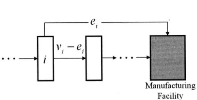
where u is the regular ordering quantity, and ei is the expediting quantity from installation

i. Note that after expediting ei from installation i, vi - ei units remain at installation i and move to installation i - 1 in the next time period as shown in Figure 2-2.

co-Manuiacturing Facility

Figure 2-2: Expediting a partial order from installation i

efficients. All presented results hold also in the nonstationary case as discussed in Section 2.5. Therefore we drop time index k from the demand variables and the cost coefficients. We also use L(-) for stationary systems instead of Lk(').

2.3

Sequential Systems

Optimality equation (2.1) is hard to analyze. To obtain analytical results, we have to confine our interest to a special class of systems. In this section, we explore systems that are analytically manageable and derive structural results for such systems. First, we formally define sequential systems using expediting costs.

Sequential systems A system is sequential, if expediting cost coefficients di's satisfy

di - di-1 5 dj+l - di for 1 < i < L - 1, where do = 0.

For sequential systems, the expediting cost coefficients are increasing convex in instal-lation i. Sequential systems can be found in situations similar to the following explanatory example. Consider a supply chain system with a supplier in Portland, Oregon and a man-ufacturing facility in Boston, Massachusetts. In between the two locations, there is an installation in St. Louis, Missouri. The review period is one week. The regular delivery lead times between the supplier and the intermediate installation and between the interme-diate installation and the manufacturing facility are one week by ground. The expedited shipment by overnight air is available from the supplier with cost d2 and the intermediate

in-stallation with cost dl. The freight air market between Portland and Boston is much weaker than the high volume market between St. Louis (a logistics hub) and Boston. Therefore, the economies of scale imply that the expediting cost can be much higher in Portland than

in St. Louis. As a result we could have d2 - dl _ dl, or equivalently d2 > 2dl.

The following is a key theorem to derive the optimal policies for regular ordering and expediting.

Theorem 1. Sequential systems preserve the sequence of orders in time when operated

optimally.

To prove this theorem, we need the following lemma proved in Appendix.

Lemma 1. For a sequential system, di d d i-j for all i and 1 < j < i - 1.

+

Proof of Theorem 1. Expediting has no lead time, thus expediting multiple units can be

decomposed to multiple decisions of expediting a unit from a certain installation, until there is no further need of expediting. Consider two nonempty installations i and

j,

j,

and the two following actions at the current time period.

Action 1: Expediting a unit from installation i

Action 2: Expediting a unit from installation

j

We show that there exists a suboptimal strategy that starts with Action 2, costs no more, but replicates the effect of Action 1. Action 1 has an effect of raising the inventory of the manufacturing facility by 1 unit for i time periods compared to no action. Similarly, Action 2 has an effect to raise the inventory for j time periods. Since installation i is nonempty, there is at least a unit, and let us denote it by A. Consider a strategy that starts with Action 2 and expedite unit A after

j

j time periods, unit A is in installation i -

j.

j

time periods and expediting unit A raises the inventory for further i -

j

Now consider the expediting cost. Action 1 costs di while the replicating strategy costs

dj + di-j. For sequential systems, Lemma 1 indicates that Action 1 is more costly or at

least of equal cost to the replicating strategy. Therefore the replicating strategy costs no more and is obviously suboptimal. The existence of the suboptimal strategy implies that any strategies that start with Action 1 cannot be optimal. In other words, if expediting is necessary in sequential systems, it is optimal to expedite from the nonempty installation that is closest to the manufacturing facility. Therefore, orders preserve sequence in time under an optimal expediting policy for sequential systems. This completes the proof. 0

In sequential systems, it is never optimal to expedite from installation i before expediting all the outstanding orders at the downstream installation of installation i. Using this fact, we formulate an alternative optimality equation equivalent to (2.1). Let x' be the sum of the inventory from installation 0 to installation i: x' = -o0vj. Let = (0,0,... ,0)

be a vector containing i zeros. For 1 < j < L, let J(.) be the optimal cost-to-go that can be achieved by a restricted control space, in which expediting from installations j + 1,j + 2,... , L in time period k is not allowed. The control space for JX is restricted in time period k, but unrestricted after time period k. Note that JL(.) = k(). We utilize

J() with respect to a fictitious state (xi-l, i-,vi, , VL-1), where installation 0 has inventory xi - 1, and installations 1, 2, -- , i- 1 are empty. The optimality equation for

Jk( ,i- I i-1

Vi***

Jk(x 1 1

, vi,.. , VL1) = mn di i - xi-1) + L(yi)

+

-1) i

-•Iyi•xizzx L- 1 _(2.2)

+

,z- xL-1),

where yi and z are decision variables: yj - xi- 1 is the expediting amount from installation i and z - xL- 1 is the regular ordering amount.

An alternative formulation of the optimality equation for Jk of sequential systems is given by

Jk(vo,

+

divi

At time period k, the first term corresponds to expediting partially or fully from installation 1 and no expediting beyond, the second term captures expediting everything from instal-lation 1, expediting partially or fully from instalinstal-lation 2, and no expediting beyond, and so forth. Since the system is sequential, the eventual optimal decisions for regular ordering and expediting are determined by the minimum term in (2.3). For example, if the j-th term achieves the minimum in (2.3), the optimal decision for expediting is to expedite all

outstanding orders in installations 1, 2, -.. - - , j- 1 and to expedite yj - x - 1 from installation

j

j.

2.4

Optimal Policies for Sequential Systems

First we introduce preliminary results needed to derive optimal policies for sequential sys-tems, and then we present main results.

Preliminaries

The following lemma from Lawson and Porteus (2000), which originates in Karush (1959), is used frequently throughout the chapter.

Lemma 2. Let

f

zl<_X<X2

h(x2) are

0

g(xi) = f0l a < y* and h(x2)

f(xi)

a

> y*

For a nondecreasing convex

f,

hand, for a nonincreasing convex

f,

In Lemma 2, g is nondecreasing convex, while h is nonincreasing convex. The following functions are required later in the derivation of the optimal policies. For 1 < i < L and k < T, let us recursively define

fi,k(x) = dix + L(x) + E[SII,k+1(x - D)], (2.4)

Sik

+t-l,k+l,

Sk(X)

gi,k(X)

-

dix,

(2.5)

Sk(x) = hi,k(x) - L(x) + E[S2jl,k+l(x - D)],

where

)

)

0 for all i.

Here,

and

defined according to Lemma 2 with respect to

firk.

fi,k and Sjk are well defined, and starting from the last time period T, they can be obtained recursively. In particular, from (2.4) we can compute fi,T, then from (2.5) we obtain S%,T1'

for all i. Next we compute fi,T-1 from (2.4), and in turn, ST %,T-1 from (2.5) for all i. We repeat this procedure to define all fi,k and Sk. For Sk and Sk we use a similar procedure.

We use the following lemma in deriving the optimal policies. The proof is provided in Appendix.

Lemma 3. a. For sequential systems, fi,k(') is convex for all k and i.

b. For all k and i we have S9k+

Skx+ S

()

= 0.

c. Let fl be convex and b e R. We have min {fi(x) + f2()} ) al + gi(b) + min{hi(y) +

b<x<y by

f2(y)}, where al, h1, and gi are defined as in Lemma 2 with respect to fl.

Let us denote by Y!k a minimizer of fi,k(): Yk = arg

min

Theorem 2. a. For sequential systems, Yi*,k's are nonincreasing in i for a fixed k. That is,

y*k Y+1,k for all i and k.

b. For sequential systems, function gi,k(x) + S2_ ,k(x) is convex for all i and k.

Optimal Policies

The optimal policies for sequential systems are given by the following theorem.

Theorem 3. For sequential systems, the following properties hold.

a. The optimal expediting policy for expediting orders from installation i is the base stock pol-icy with respect to echelon stock x'. The base stock level is given by Yi*,k = arg min fi,k (X) for time period k.

b. The optimal regular ordering policy is the base stock policy with respect to inventory position xL- 1. The base stock level is given by z* = argmin{hL,k

(z) +cz+E[

-D) + Hk+1(Z - D)]} for time period k, where Hk(x) follows Hk(x) = min{hL,k(Z) + cz +

E[S + Hk+(z - D)] -1,k+1(Z - D) Sk(z>x) - cx, and HT () = 0

c.

For

Jk(X

i-1, I, ,VL-1)-Jk i iVi+1, . , VL-1) = k+Sk 1

,k

(xi).

Part (a) of Theorem 2 indicates that the expediting base stock levels are nonincreasing in i. On the other hand, echelon stock x' is nondecreasing in i, thus there exists only one i* such that Yi*,k - xi*-1 > 0 and Yi*+l,k - xi* < 0. From part (a) of Theorem 3 we conclude that the optimal expediting policy is to expedite everything from installations 1, -.. - - , i* - 1, and partially from installation i*, and nothing beyond. This sequential expediting structure agrees with Theorem 1.

Additionally, the following lemma is used in the proof of Theorem 3. This lemma is proved concurrently with Theorem 3 in an induction step as shown below.

Lemma 4. For sequential systems,

a. Hk(x) = Jk(x, 6L-1), _and

b. S2 1,k(X)

+

Proof of Theorem 3 and Lemma 4. We prove Theorem 3 and Lemma 4 by induction. In the base case of the induction, when k = T + 1, the optimal expediting policy and the optimal

regular ordering policy are null. We can safely set the base stock levels for expediting and regular ordering at -oo. Also, part (c) of Theorem 3 and all the properties in Lemma 4 trivially hold when k = T + 1 because they are all zero.

Now we continue with the induction step. Let us assume that on and after time k + 1 <

T + 1, the theorem and the three properties hold. Note that we only need to show the

results at time period k.

First, we prove part (a) of Lemma 4. Consider JL(XL-1 0L-1) in (2.3) which is the

same as Jk(xL - 1, 0L-1). Vector (xL-1, 6L -1) is a state in which we may expedite YL - x

L - 1

only from the supplier up to the amount of the regular order z - xL- 1 because there is no outstanding order in any installation. The recursive relationship from (2.2) with i = L is

Jk(XL-, oL -1)

S in {dL(YL - xL-1) + L(yL) + c(z - xL-1) + E[Jk+1(YL - D, 6L-2 z- YL)]}

- mmin {dL(YL - xL -l) + L(yL)

+

xL- 1 _ +_YLZ

where we use part (c) of Theorem 3 for time period k + 1. Using the definition of fL,k and part (c) of Lemma 3, we have

Jk(XL-1 L-1) ) = min {fL,k(YL)

+

+ Sl-1,k+1 - dLxL - 1 _ cxL - 1

- min hL,k(z) + cz + E[S L-l,k+l(z - D) + Jk+l(z - D,0L1 )]} (2.6) xL l<z

+

Rearranging the terms and using part (b) of Lemma 3 lead to Jk(xL -_1, L -_{1) =}

mmin {hL,k(z)+

XL-l <z

cz + E[S2-1,k+l(z - D) + Hk+1(z - D)]} - S2,k(XL - 1) - cxL -l, which is the definition of

Hk(xL- 1). Therefore, part (a) of Lemma 4 is proved.

Next, we prove part (b) of Lemma 4. From (2.6) and part (a) of Lemma 4, we have

Sl,k(x L-1) + Hk(xL - 1) = min {hL,k(z)

+

xL-l<z

+

+

Because gL,k(XL -1) + S2-1,k(XL -_{l) is convex by part (b) of Theorem 2, and S2l,k+l(Z} -D) + Hk+1 (z - D) is convex by the induction hypothesis, we conclude that SL2_l,k(x L

-l) +

Hk(xL -l) is convex. This shows that part (b) of Lemma 4 holds.

Now we prove part (a) of Theorem 3. Let us consider (2.2). By applying part (c) of Theorem 3 with time period k + 1 to Jk+l(yi - D, Oi-2,xi - yi, vi+l, "" , Z - XL -1l) in (2.2), we obtain Jk+l(yDi - D, - Yi,vi+l, . ,z - XL -1 SO1,k+

+

S21,k+l ( i- D) + Jk+ (xi -D, Wi-1, vi+l, . , z - XL- 1). Applying this repeatedly, we have Jk+ l(X - DOi - 1, Vi+1, 1 ,z - XL -1) L-2 -_ D) +1 E2 +S X3-D -Sil,k+l SS-1,k+ (Yi -,k + i - D) ?{Skk+ - D) + + S(,k+1(xk - D) j=i + Sj,k+l xj+ - D)} + Jk+l (XL-- D, L-2 L-1 L-2 __SO - D)+1> S i-

Sl,k+1 + Si-l,k+l (Yi - D) + Sl?-1,k+1(xi- D) + Z{S,k+1 + Sk+l(x - D)

j=i

" Sk+l j+' - D)}

+

+

Substituting this into (2.2) yields

Jk(xi- ,i- ,vi,... , VL-1) =

mmi

{d

yi

+

+

+

z>xL- 1

L-2

(2.7)

+ Si-1,k+l + E[S-1,k+1 (xi - D)] + E Z{SEk+1 + SJ,k+l(x3 - D)

j=i

+

+

From (2.7), the optimal expediting amount from installation i at time k is determined from

mm {diyi L(yi)

+

xi-l<yi<x x_ z-1•ixi

By part (a) of Lemma 3,

fi,k

argmin fi,k(yi). Note that we can only expedite up to what we have in installation i. This completes the proof of part (a) of Theorem 3.

Next, we proceed to prove part (b) of Theorem 3. We consider the optimal regular ordering policy. If the last term in (2.3) attains the minimum, then it is determined by (2.6), or equivalently

min {hL,k(z) + cz + E[SL-l,k+l(z- D) + Jk+l(z- D, L-1)]}, (2.8)

or otherwise from (2.7) it is determined by

min {cz + E[S2_l,k+l(z - D) + Jk+l(Z- D, OL-1)]}. (2.9)

z>xL- 1

Note that hL,k(z) is nonincreasing convex and hL,k(z) = 0 for z > yk Therefore, if

z > Y*,k, then (2.8) and (2.9) lead to the same minimizer z*. If z < yik, from part (a)_{k-- LkkI k L,k ,}

of Theorem 2, we have z* < yk for all i, which results in expediting everything in the supply chain including the fresh regular order in the current time period. In this case, (2.8) determines the regular ordering quantity because we are now expediting from the supplier. As a result, (2.8) determines the optimal regular ordering in any case.

Since S~Ll,k+l(z) + Hk+1(z) is convex by part (b) of Lemma 4, and Jk+l(z, L-_{1) =} Hk+1(z) by part (a) of Lemma 4, hL,k(z) + cz + E[SL_₁,k+1(z - D) + Jk+l(z - D,

OL-

Hk is well defined since hL,k(z) + cz + E[SLi-1,k+l(z - D) + Hk+1(z - D)] is convex for all

k. The proof of part (b) of Theorem 3 is thus completed.

It remains to show part (c) of Theorem 3 in time period k. Since we know optimal policies in time period k in an induction step, we use the optimal policies in proving this part. We compare Jk(x I i, Vi+1, - ' , VL-1) and Jk(xi+l, Oi+1 , vi+2, - , VL-1). If Yi+1,k • xi, then no

expediting is necessary from installation i + 1 and beyond, therefore

Ak(X i0Z Vi+l, Vi+2, " " " , VL-1)

= L(x')

+

+ E[Jk+l(X

' " V - , - L 1 ]

z>xL_l₁

= L(xi) + min {c(z - XZ>_XL - 1 L -l) + E[Sk+l + Sik+l(x - D) + Sk+kl 1 (X+1 - D)]

+ E[Jk+l (xi +1 - D, Oi , vi+2, • • • , VL-1, Z- XL - 1) ]} ,

where we used part (c) of Theorem 3. Since y*+1,k X i < i+1, no expediting is necessary, thus we have

Jk(Xi+1, i+1, Vi+2, , VL-1)

= L(x i + 1) + mmin {c(z - xL- 1) + E[Jk+l(xi+l - D,Oi,vi+2,... VL-1, Z - xL-1)]}.

Therefore, Jk(xi i, Vi+l, vi+2,'' , VL-1)-Jk(xi + •(i+1, Vi+2, " , VL-1) L(xi)-L(xi+1)

E[S(k+l + Sk+1 W - D) + Sk - D)].

Next, if xi < Yi*+1,k < i + 1 , then expediting from installation i + 1 is necessary, but not from upstream installations. We have

Jk(x , ,OI,Vi+l,Vi+2,. ,VL-1) = di+l(y*+l,k - x2) + L(y*+l,k)

+

L

-l)

z>xL-1

+

D,

,z

xL-1)]}

di+1(Yil+,k - xi) + L(yi+1 ,k) + in {c(z - XL -l) + E[Sk+l + Sik+1(Yi+1,k - D) z>xL-1

SSik+l - D)] + E[Jk+1+l - D i,vi+2,* -,VL- 1,Z - xL-1)]}, and

Jk(Xi+l,o i+l, Vi+2, ,VL-1) - L(x i +

l) + mmi {c(z - xL -l)

z>xL-1

+ E[Jk+l(xi +

l - D, ivi+2, ' ,VL-1, Z- XL-1

Therefore,

+ L(y*+lk) - di+l_{Finall,k ifk~ y*k~} xi - L(x_xy*+i + 1i +l) + E[SOk+l + S1k+1 (+1,k - D) + S k+l(xi +l - D)].

Finally, if y+,k > i+1, then we expedite everything in installation i + 1. Thus the only cost difference is d±vi+lVi di+1ix+1-di+1ix, and we obtain Jk(X, i, vi+1, vi+2, L-1)-Jk(Xi+l, Oi+1, Vi+2, , VL-1) = di+1x

i +

l - di+x1 . The three cases above can be summarized as

Jk(X, i, Vi+li+2, , VL-1) - Jk(X i+, i+1, Vi+2, * , VL1)

-=ai+1,k 9+i+1,k(Xi) + hi+l,k(Xi + 1) -- di+lxi

- L(x i+1) + Si k +l + E[Sik+ l(xi + 1 - D)] Q9S (Xi ) +4 SY2 (Xi+1)

= S+l,k + Sl+1,k(x) + S2 l,k ).

Therefore, part (c) of Lemma 4 at time period k is proved. This completes the induction step of the entire proof.

A Numerical Example of the Policy

Consider a supply chain system with 6 installations including the supplier and the man-ufacturing facility. Figure 2-3 illustrates the mechanism behind the base stock policy for regular ordering and the base stock policies for expediting. Note that the echelon stock x' is nondecreasing in i, and yk is nonincreasing in i by part (a) of Theorem 2. Therefore,