Normalized particle size distribution for remote sensing application

HAL Id: hal-00979328

https://hal.archives-ouvertes.fr/hal-00979328

Submitted on 23 Apr 2016

HAL is a multi-disciplinary open access

archive for the deposit and dissemination of

sci-entific research documents, whether they are

pub-lished or not. The documents may come from

teaching and research institutions in France or

abroad, or from public or private research centers.

L’archive ouverte pluridisciplinaire HAL, est

destinée au dépôt et à la diffusion de documents

scientifiques de niveau recherche, publiés ou non,

émanant des établissements d’enseignement et de

recherche français ou étrangers, des laboratoires

publics ou privés.

Julien Delanoë, Andrew J. Heymsfield, Alain Protat, Aaron Bansemer, R. J.

Hogan

To cite this version:

Julien Delanoë, Andrew J. Heymsfield, Alain Protat, Aaron Bansemer, R. J. Hogan. Normalized

par-ticle size distribution for remote sensing application. Journal of Geophysical Research: Atmospheres,

American Geophysical Union, 2014, 119 (7), pp.4204-4227. �10.1002/2013JD020700�. �hal-00979328�

RESEARCH ARTICLE

10.1002/2013JD020700

Key Points:

• This study describes a normalization technique to represent the PSD • In situ measurements are covering a

large variety of ice clouds

• This new data set also includes direct measurements of IWC

Correspondence to:

J. M. E. Delanoë,

julien.delanoe@latmos.ipsl.fr

Citation:

Delanoë, J. M. E., A. J. Heymsfield, A. Protat, A. Bansemer, and R. J. Hogan (2014), Normalized particle size distri-bution for remote sensing application,

J. Geophys. Res. Atmos., 119, 4204-4227,

doi:10.1002/2013JD020700.

Received 7 AUG 2013 Accepted 13 JAN 2014

Accepted article online 15 JAN 2014 Published online 14 APR 2014

Normalized particle size distribution for remote

sensing application

J. M. E. Delanoë1_{, A. J. Heymsfield}2_{, A. Protat}3_{, A. Bansemer}2_{, and R. J. Hogan}4

1_{LATMOS/UVSQ/IPSL/CNRS, Guyancourt, France,}2_{NCAR, Boulder, Colorado, USA,}3_{Centre for Australian Weather and}

Climate Research, Melbourne, Victoria, Australia,4_{Department of Meteorology, University of Reading, Reading, UK}

Abstract

The ice particle size distribution (PSD) is fundamental to the quantitative description of a cloud. It is also crucial in the development of remote sensing retrieval techniques using radar and/or lidar measurements. The PSD allows one to link characteristics of individual particles (area, mass, and scattering properties) to characteristics of an ensemble of particles in a sampling volume (e.g., visible extinction (𝜎), ice water content (IWC), and radar reflectivity (Z)). The aim of this study is to describe a normalization technique to represent the PSD. We update an earlier study by including recent in situ measurements covering a large variety of ice clouds spanning temperatures ranging between −80◦C and 0◦C. This new data set also includes direct measurements of IWC. We demonstrate that it is possible to scale the PSD in size space by the volume-weighted diameter Dmand in the concentration space by the intercept parameter N∗0and obtain

the intrinsic shape of the PSD. Therefore, by combining N∗

0, Dm, and a modified gamma function representing

the normalized PSD shape, we are able to approximate key cloud variables (such as IWC) as well as cloud properties which can be remotely observed (such as Z) with an absolute mean relative error smaller than 20%. The underlying idea is to be able to retrieve the PSD using two independent measurements. We also propose parameterizations for ice cloud key parameters derived from the normalized PSD. We

also investigate the effects of uncertainty present in the ice crystal mass-size relationships on the parameterizations and the normalized PSD approach.

1. Introduction

Remote sensing instruments give us the potential to tackle issues such as the role of clouds in climate and also the cloud processes involved. These instruments, active or passive which can be located on different platforms, require critical assumptions to convert raw measurements into cloud properties. Most retrieval techniques use lookup tables or empirical relationships to link measured parameters to microphysical cloud properties, either through a retrieval process or an instrument simulator. The particle size distribu-tion (PSD) of ice cloud particles can be defined as the concentradistribu-tion of ice particles as a funcdistribu-tion of their maximum dimension. It allows one to characterize the particles per unit of volume and their bulk proper-ties. For instance, it is straightforward to calculate the ice water content (IWC) from the combination of the mass as the function of the maximum dimension (hereafter M(D), where D is the maximum dimension of the ice crystal as derived by finding the minimum diameter of a circle that fully encloses the two-dimensional image of a particle) of a particle and the PSD. The characterization of the PSD is a challenging task since it greatly depends on meteorological conditions and location.

Some recent combined radar and lidar retrieval techniques use the normalized PSD approach [Delanoë et al., 2007; Delanoë and Hogan, 2008, 2010; Szyrmer et al., 2012] to simplify the relationships between cloud prop-erties and instrument measurements such as radar reflectivity or Doppler velocity. This paper aims to update the work of Delanoë et al. [2005], by considering direct measurements of the IWC, yielding progresses made with microphysical probes knowledge of M(D).

We also propose a new technique to estimate the optimal intrinsic shape of the PSD by minimizing the dif-ferences between moments of the PSD, such as visible extinction and radar reflectivity, calculated from the normalized and the non-normalized approach.

In section 2, we present the normalized PSD concept for ice clouds. A description of the data and the main microphysical assumptions involved in the study is given in section 3. The impact of the normalization on the PSD, the cloud variables (such as IWC, extinction, and such) as well as cloud properties which can

be remotely observed (such as radar reflectivity or the terminal fall velocity) is described in section 4. We propose a parameterization for the normalized PSD and key cloud variables and its assessment in sections 5 and 6. We will then conclude and discuss the results in the last section.

2. The Normalized Particle Size Distribution Concept

In this section we summarize the normalized PSD concept of Delanoë et al. [2005]. In order to adapt the framework introduced by Testud et al. [2001] for rain drop spectra to the case of ice particles, Delanoë et al. [2005] used the equivalent melted diameter (D_eq). Using this framework, D_eqcan be then be calculated using the following relationship:

Deq= [ 6 M(D) π𝜌_w ]1 3 [m], (1)

where𝜌wis the density of water (1000 kg/m3). By definition Deq ≤ D, the particle, once melted, cannot be

larger than its maximum diameter. It would correspond to an ice density exceeding the density of solid ice (917 kg/m3_{), which is obviously not possible.}

M(D) is commonly represented using a power law relationship and derived using PSD spectra combined with bulk measurements of IWC [Brown and Francis, 1995; Lawson and Baker, 2006; Heymsfield et al., 2010]. The mass-size relationship used in Delanoë et al. [2005] study came from Brown and Francis [1995], employ-ing a very limited data set. For instance, the observations reported by Brown and Francis [1995] were acquired primarily at temperatures from −20◦C to −30◦C, with masses dominated by particles in the 200–800 micron size range. Although this relationship can be applied to many kinds of ice clouds [Heymsfield et al., 2010] and it is still used in many radar-lidar retrieval algorithms [Delanoë and Hogan, 2008, 2010], it may not be the most appropriate relationships for all ice clouds met in this study. Therefore, we used the dedicated mass-size relationships developed from direct IWC measurement and provided in Heymsfield et al. [2010]. These relationships will be described later on in the data description section 3.3. The particle size distribution N(D) can also be rewritten in terms of Deqas by definition Neq(Deq)dDeq = N(D)dD for a given diameter bin. Ice water content is therefore proportional to the third moment of Neq(Deq): IWC = π𝜌w 6 ∫ ∞ 0 N(Deq)Deq3dDeq, (2)

The basis of the normalized approach is to scale both diameter and concentration (extensive variable) parameters, and it was introduced by Sekhon and Srivastava [1971] for the drop size distribution. They used the median volume diameter and a number density as scaling parameters. However, a specific shape was assigned to the drop size distribution to link the scaling parameters; the normalization was considered as a single-moment normalization. This constraint was released by Testud et al. [2001], who showed that it was not necessary to fix the drop size distribution shape. Later on, Lee et al. [2004] demonstrated that it was possible to normalize the PSD using different combinations of moments of the particle size distribu-tion. Therefore, the choice of parameters which scale the concentration and the diameter is crucial. As the water content remains a key variable for clouds, it appeared therefore useful to make the normalized PSD independent from this variable.

Testud et al. [2001] and Delanoë et al. [2005] defined the mean volume-weighted diameter as the ratio of the fourth and the third moments of the PSD in terms of Deq(note that the third moment corresponds to

LWC or IWC): D_m=∫ ∞ 0 N(Deq)Deq4dDeq ∫∞ 0 N(Deq)Deq3dDeq . (3)

Assuming that the number concentration can be scaled by a normalization factor called N∗

0, we can write

where the function F in (4) represents a mathematical function and will be described in detail later in the paper. F will be referred to as the “shape” of the distribution in the following. If we replace N(D_eq) in (3) by equation (4), we obtain D_m= ∫ ∞ 0 N∗0F(Deq∕Dm)Deq4dDeq ∫∞ 0 N ∗ 0F(Deq∕Dm)Deq3dDeq . (5) Then we define X as X = Deq∕Dm, (6)

and we rewrite expression (5) in terms of X

Dm= D5 mN0∗∫ ∞ 0 F(X)X4dX D4 mN0∗∫ ∞ 0 F(X)X3dX . (7)

After simplifications, (7) leads to

∫ ∞ 0 F(X)X4_{dX = ∫} ∞ 0 F(X)X3dX = C, (8)

where C is a constant. Combining (2), (4), and (8), IWC can be expressed as a function of N∗ 0and Dm: IWC = π𝜌w 6 N ∗ 0D 4 mC. (9)

Cwas arbitrarily chosen by Testud et al. [2001] to be equal to Γ(4)∕44_{and to correspond to the intercept}

parameter of an exponential distribution. N∗

0follows therefore an expression of the form

N∗₀= 4 4 π𝜌_w IWC D4 m [m−4]. (10)

And in terms of moments of the equivalent PSD

N∗ 0= 44 6 [ ∫∞ 0 N(Deq)Deq3dDeq ]5 [ ∫∞ 0 N(Deq)Deq4dDeq ]4[m −4_{]. (11)}

The function F in (4) is the “unified” size distribution shape given by Delanoë et al. [2005] and has been found to fit measured size distributions when they are appropriately normalized and can be described as

F(𝛼, 𝛽, X) = 𝛽Γ(4) 44 Γ(𝛼+5 𝛽 )4+𝛼 Γ(𝛼+4 𝛽 )5+𝛼X𝛼exp ⎡ ⎢ ⎢ ⎢ ⎣ − ⎛ ⎜ ⎜ ⎜ ⎝ X Γ(𝛼+5 𝛽 ) Γ(𝛼+4 𝛽 ) ⎞ ⎟ ⎟ ⎟ ⎠ 𝛽 ⎤ ⎥ ⎥ ⎥ ⎦ , (12)

where𝛼 and 𝛽 allow one to adjust the shape to the measured normalized PSD. Delanoë et al. [2005] esti-mated the𝛼 and 𝛽 coefficients for the modified gamma shape using in situ data base. Unfortunately, the data set used in that study did not include direct IWC measurements, which made it impossible to find an optimal M(D). In addition to that, this data set did not adjust the PSD to account for shattering of small particles.

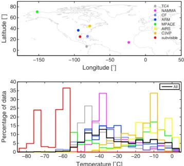
−150 −100 −50 0 50 0 20 40 60 80 Longitude [°_] TC4 NAMMA CF ARM MPACE AIRS C3VP subvisible −80 −70 −60 −50 −40 −30 −20 −10 0 0 5 10 15 20 25 30 35 40 Temperature [°_C] Latitude [ °] Percentage of data All

Figure 1. Probability distribution of the data as a function of temperature, for (top) each field campaign (TC4, NAMMA,CRYSTAL-FACE, ARM, C3VP, AIRS, and Subvisible) and (bottom) the whole data set.

3. Data Description

3.1. Presentation of the Data

In this study we used midlatitude, high-latitude, and low-latitude data sets. The data are described in detail in Heymsfield et al. [2013]. Midlatitude data are from the Atmospheric Radiation Measurement (ARM) 2000 campaign, an intensive observing period including three cold cirrus cloud flights in synoptically gener-ated ice clouds over Oklahoma. Convectively genergener-ated tropical cirrus and anvil data from Florida are from citation aircraft from CRYSTAL-FACE (Cirrus Regional Study of Tropical Anvils and Cirrus-Layers-Florida Area Cirrus Experiment). These data were collected in 2002 and also include very cold temperature cirrus sam-pled by the WB57F aircraft during CRYSTAL-FACE and will be referred to as Subvisible in the text. Subvisible also includes data from one WB57F aircraft flight between Houston and Costa Rica during the Pre-Aura Validation Experiment; more details can be found in Schmitt and Heymsfield [2009].

More recent tropical data are also included in this study. NAMMA (NASA African Monsoon Multidisciplinary Analyses, http://airbornescience.nsstc.nasa.gov/namma/) campaign, which took place in Western Africa in 2006, provided a dozen convectively generated ice and mixed-phase clouds. Some convectively gener-ated ice clouds sampled near Costa Rica in 2008 from the TC4 (Tropical Clouds, Convection, Chemistry, and Climate) [Toon et al., 2010] campaign are also included in the study. Synoptically generated ice cloud lay-ers with embedded convection and supercooled liquid water are from the Alliance Icing Research Study II (AIRS-2); there were seven flights over the Toronto area [see Isaac et al., 2005]. The study also includes three flight data collected in 2006–2007 during the CloudSat/CALIPSO validation Project (C3VP) in the area of Montreal, Canada. Arctic data are from the Mixed-Phase Arctic Cloud Experiment (M-PACE) [Verlinde et al., 2007], 13 flights in Prudhoe Bay, Alaska, area. The locations where the campaigns took place are presented in Figure 1 (top). Note that air temperatures for all field programs were measured with a Rosemount tem-perature probe. The distribution of the data as a function of temtem-perature is depicted in Figure 1 (bottom). The black line, which represents the full data set, shows that most of the data spans between −50◦C and 0◦C with a few data collected at very cold temperatures. TC4 and NAMMA data show a monomodal dis-tribution with peaks at −45◦C and about −40◦C, respectively. On the other hand, CRYSTAL-FACE and ARM have a flatter distribution with no obvious peaks. The M-PACE measurements correspond to both very cold clouds (colder than −40◦C) and clouds between −20◦C and 0◦C where we occasionally detected the pres-ence of supercooled water (discussed later). The C3VP and AIRS data were collected in warm ice clouds with a peak centered at −10◦C for C3VP and ice clouds not colder than −40◦C. The coldest ice particles are from “Subvisible” with temperatures spanning from −80◦C to −60◦C.

Table 1. Number of 5 s PSD Used in the Study for Each Campaign and Its Percentage of Whole Data

Campaign Number of 5 s PSD Used in the Study Percentage of Whole Data

TC4 13,779 25 NAMMA 9,315 16.8 CRYSTAL-FACE 11,966 21.7 ARM 6,187 11.2 M-PACE 2,368 4.3 C3VP 3,348 6 AIRS 7,867 14.2 Subvisible 455 0.8

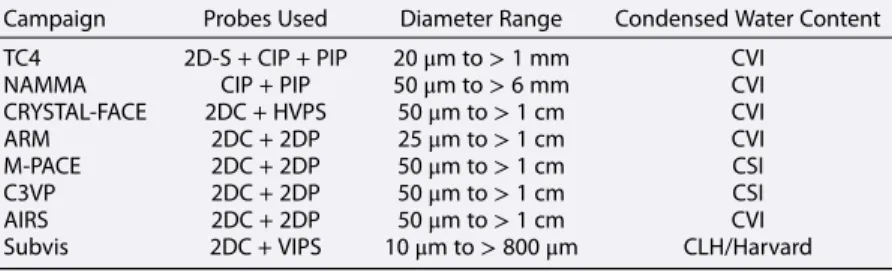
PSDs were acquired using the following probes, including: 2-D-Cloud and Precipitation (2DC-2DP) probes, Droplet Measurement Technologies Precipitation Imaging Probes (PIP), and High Volume Precipitation Spectrometer (HVPS). The number of 5 s PSD used in the study is recalled for each campaign in Table 1. Probe combinations and diameter ranges for each field campaign are given in Table 2. For the Subvisible data set, data were also collected from a video ice particle sampler [Schmitt and Heymsfield, 2009]. A two-dimensional stereo (2D-S) probe was also used for the TC4 analysis (10 μm to> 1 mm). Total condensed water contents (TWC), ice plus liquid when present, were measured with a Counterflow Virtual Impactor or a Cloud Spectrometer and Impactor (CVI and CSI, respectively) for TWC> 0.01 g m−3_.

Direct measurements of ice water content above a lower cutoff particle diameter of about 6 μm were obtained from the Counterflow Virtual Impactor (CVI) [Twohy et al., 1997] and a related Cloud Spectrome-ter and Impactor (CSI) probe. The overall uncertainty of the CVI is about 13% at waSpectrome-ter contents of 0.05 to 1.0 g m−3_{. Uncertainty increases to 16% for the minimum detectable IWC of about 0.01 g m}−3_{. The probe is}

saturated at IWCs above about 2 g m−3_{[Twohy et al., 1997]. IWC for the Subvisual data set was measured by}

the University of Colorado closed-path tunable diode laser hygrometer (CLH) for CRYSTAL-FACE.

3.2. Data Processing and Quality Control

In situ data required extensive processing and quality control. For instance, the 2-D probe PSD data are pro-cessed to account for ice shattering using particle interarrival times [see Field et al., 2006]. Because of the ice shattering issue, the Forward Scattering Spectrometer Probe or Cloud and Aerosol Spectrometer probes data are not used for small particles. Heymsfield et al. [2013] justified this approach by comparing the PSDs with and without the small-particle data to observations from the 2D-S probe from TC4. The impact of the shattering effect is investigated in section A1. Liquid water could artificially increase extinction and influ-ence the ice PSD. In the data set, liquid water was detected and its content estimated from a Rosemount Icing Probe. Liquid water encounters were infrequent and have been filtered out of the data set. The min-imum diameters used in this study are 50 μm (TC4/NAMMA/M-PACE/ARM/CRYSTAL-FACE/C3VP/AIRS). The impact of not using particles below 50 μm is discussed in section A2 using 2D-S TC4 data. The Subvisible data are the only data set using ice particle data below 50 μm. This is warranted for two reasons. First, the measurements are made with a probe with a relatively large sample volume for small particles and directly captures the particles and images them rather than with other instruments. The second reason is that at the

Table 2. Probes Used in Each Campaign and Diameter Ranges Available

Campaign Probes Used Diameter Range Condensed Water Content

TC4 2D-S + CIP + PIP 20μm to>1 mm CVI

NAMMA CIP + PIP 50μm to>6 mm CVI

CRYSTAL-FACE 2DC + HVPS 50μm to>1 cm CVI

ARM 2DC + 2DP 25μm to>1 cm CVI

M-PACE 2DC + 2DP 50μm to>1 cm CSI

C3VP 2DC + 2DP 50μm to_>1 cm CSI

AIRS 2DC + 2DP 50μm to>1 cm CVI

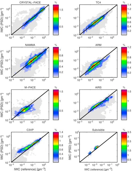
IWC (PSD) [gm −3 ] CRYSTAL−FACE 10−3 10−2 10−1 100 10−3 ₁₀−2 ₁₀−1 ₁₀0 10−3 ₁₀−2 ₁₀−1 ₁₀0 10−3 10−2 10−1 100 10−3 10−2 10−1 100 IWC (PSD) [gm −3 ] 10−3 10−2 10−1 100 IWC (PSD) [gm −3 ] 10−3 10−2 10−1 100 10−3 10−2 10−1 100 10−3 ₁₀−2 ₁₀−1 ₁₀0 10−3 ₁₀−2 ₁₀−1 ₁₀0 10−3 10−2 10−1 100 10−3 10−2 10−1 100 10−3 10−2 10−1 100 10−3 10−4 10−2 10−1 100 IWC (PSD) [gm −3 ] 10−3 10−2 10−1 100 % 0.5 1 1.5 TC4 % 0.2 0.4 0.6 0.8 1 1.2 1.4 NAMMA % 0.2 0.4 0.6 0.8 1 ARM % 0.2 0.4 0.6 0.8 1 1.2 M−PACE % 0.5 1 1.5 AIRS % 0.5 1 1.5 IWC (reference) [gm−3_] C3VP % 0.2 0.4 0.6 0.8 1 1.2 1.4 IWC (reference) [gm−3] IWC (PSD) [gm −3 ] Subvisible 10−4 10−3 10−2 10−1 100 % 0.5 1 1.5 2 2.5 3 3.5

Figure 2. Probability distribution plots of IWC calculated from the PSD as a function of the reference IWC derived from CSI, CVI, or equivalent, for each field campaign (CRYSTAL-FACE, TC4, NAMMA, ARM, M-PACE, C3VP, AIRS, and Subvisible).

very low temperatures associated with the Subvisible data, it is likely that the small particles are numerous compared to warmer temperatures.

3.3. Mass and Area Relationship Assumptions for the Calculation of Cloud and Observed Variables

As noted earlier, the mass-size relationship assumption is crucial when we apply the normalized PSD approach as we need to compute the equivalent melted diameter. Fortunately, in situ data involved here contain CVI, CSI, or equivalent measurements which allow one to measure IWC with only a few assumptions and this IWC will serve as a reference, hereafter IWCref. Note again that no bulk measurement was available

in the Delanoë et al. [2005] study.

In our study we used different M(D) described in Heymsfield et al. [2010] which are based on direct mea-surements of the IWC. These M(D) have been combined with the particle size distribution to derive several IWC estimates. We selected the M(D) which gave us a better match to IWCreffor each campaign. The best M(D) will be referred to as the "retrieved" M(D) in our study. As mentioned in Heymsfield et al. [2010], each mass-size relationship was derived for specific cloud conditions, for instance: “vicinity of deep convection,”

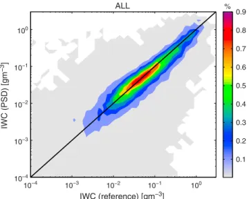
IWC (reference) [gm−3] IWC (PSD) [gm −3 ] ALL 10−4 10−3 10−2 10−1 100 10−4 10−3 10−2 10−1 100 % 0.1 0.2 0.3 0.4 0.5 0.6 0.7 0.8 0.9

Figure 3. Same as Figure 2 for the whole data set (TC4, NAMMA, CRYSTAL-FACE, ARM, C3VP, AIRS, and Subvisible).

“convectively generated,” “warm,” or “composite” (including different sort of clouds). The results of the IWC comparison are presented in Figures 2 and 3, which show the probability distribution of the IWC computed using the measured PSD and IWC_reffor each campaign and all the campaigns, respectively. Note that we have removed all the data contaminated by liquid water (see section 3.1). It is clearly demonstrated that the mass relationships selected (Table 3) are in good agreement with IWC_ref; most of the data are concentrated in the 1:1 region of the scatterplots, and the selected relationships do not seem to introduce any bias in the derived IWC. The best results are obtained for CRYSTAL-FACE and TC4 data, while NAMMA, ARM, and M-PACE values are more scattered. Accordingly, we will use in our calculation the composite M(D) for TC4, ARM, and M-PACE, the relationship obtained for convectively generated cloud for CRYSTAL-FACE, the relationship for clouds in vicinity of deep convection for NAMMA, and the warm cloud relationship for C3VP. Note that the composite relationship is perfectly suitable for at least three campaigns and only CRYSTAL-FACE, NAMMA, and the Subvisible require more specific relationships. We will also compute the visible extinction param-eter, and therefore, we also need to be able to derive the cross-sectional area of particles of each given diameter [Heymsfield et al., 2013]. It is directly computed from the projected area of the particle.

The sampled maximum chord length diameter of a given particle is used to define its diameter. The particle “area ratio” is derived from the images areas for each particle normalized by the area of an equivalent diam-eter circle. Statistics on particle area ratios per size bin are compiled over 5 s intervals. For each size bin and for each 5 s interval, an average area ratio is derived.

Deriving M(D) is clearly an advantage; however, we also need to analyze the impact of commonly used relationships applied to the whole data set. Therefore, we decided to select one of them which is currently used in the radar-lidar DARDAR products (http://www.icare.univ-lille1.fr/projects/dardar/) combining

Table 3. Mass-Size Relationships Used for Each Campaign

Campaign Names Relationships (cgs)

TC4 Composite M(D) = 7e−3_D2.2

NAMMA Vicinity of deep convection M(D) = 11e−3_D2.1

CRYSTAL-FACE Convectively generated M(D) = 6.3e−3_D2.1

ARM Composite M(D) = 7e−3_D2.2

M-PACE Composite M(D) = 7e−3_D2.2

C3VP Warm M(D) = 3.59e−3D2.1

AIRS Composite M(D) = 7e−3_D2.2

Subvisible Specific M(D) = 16_.39e−3_D2.49

CloudSat and CALIPSO measurements [Delanoë and Hogan, 2010]. This is motivated by the fact that the M(D) assumed in the retrieval technique is a combination of two relationships of Brown and Francis [1995] for D>300 μm and Mitchell [1996] for hexagonal columns. Note that Brown and Francis [1995] mass-size relationship has been widely used and evaluated in Heymsfield et al. [2010].

DARDAR mass-size relationships are given below (cgs):

M(D) = 1.677 e−1_D2.91 _{D<= 0.01 cm (13)} M(D) = 1.66 e−3_D1.91 _{0.01 < D <= 0.03 cm (14)}

M(D) = 1.9241 e−3D1.9 D> 0.03 cm (15)

Note that (15) has been modified, assuming an aspect ratio of 0.6 [Hogan et al., 2012] to convert the mean diameter to maximum diameter. This adapted mass-size relationship is used in this study and will be referred to as “DARDAR.”

In this study we will compute IWC, N∗

0, Dm, the radar reflectivity factor at 94 GHz (Z), the terminal fall

veloc-ity (Vt), and the effective radius (re) using the retrieved M(D) and in section 5.4, we will add DARDAR M(D).

As a rough approximation, the reflectivity factor can be assumed to be proportional to the sixth moment of the PSD. However, this simplification is not valid at 94 GHz for large particles so the reflectivity is com-puted using the T-matrix approach, particles are assumed to be spheroids, and the mass-size relationship is used to calculate the fraction of ice included in the spheroid and the dielectric factor. The T-matrix approach requires the knowledge of the aspect ratio of the particles; as a matter of consistency, we assume a ratio of 0.6 [Hogan et al., 2012]. Reflectivity weighted terminal fall velocity is computed using Heymsfield and Westbrook [2010]. Note that visible extinction and terminal fall velocity are derived using the particle size distribution and the cross-sectional area of the particles as a function of their diameter. From IWC and the visible extinction, we can compute the effective radius:

r_e=3 2

IWC 𝜎𝜌i

, (16)

where𝜌iis the density of solid ice and𝜎 is the visible extinction Foot [1988].

4. Impact of the Normalization

4.1. Impact on the PSD

PSDs from each field campaign are derived in term of equivalent melted diameter using equation (1) and the mass-size relationship identified earlier (section 3.3), and for each spectrum, N∗

0and Dmare also

com-puted. Figure 4 shows the impact of the normalization, where contours illustrate the distribution of the data in both configurations: raw (left) and normalized (right) spectra. The impact of the normalization is obvi-ous, data are concentrated in a smaller area, and sampling effects are reduced. NAMMA and CRYSTAL-FACE non-normalized spectra exhibit a large scatter with several orders of magnitude in concentration for a given diameter. This is probably due to the fact that the data are sampled in convectively generated ice clouds. The maximum number of hits is about 0.4–0.5% while the maximum of data, once normalized, reaches more than 1.2% and spans only a few orders of magnitude in concentration for a given Deq∕Dm.

The raw TC4, ARM, M-PACE, C3VP, and AIRS spectra, despite a wide range of values in number concentration, show green peaks (0.5%) at around 102_m−3_μm−1_{, but the variability in concentration clearly decreases after}

normalization. Subvisible data span a smaller range of diameters; this is expected due to the very cold tem-peratures and the nature of the sampled clouds. The raw concentration remains largely variable (i.e., several orders of magnitude), and the impact of the normalization is noticeable.

The effect of the normalization is important for each spectrum, while the raw spectra had different pat-terns and differences in the distribution of the concentration the normalized spectra show very similar shapes. Most of the data are concentrated in the area where D_eq∕D_m = 1, even for Subvisible data, and normalized PSDs will differ from their wings around this value. Delanoë et al. [2005] and Field et al. [2007] showed that as a function of the field campaign location, the shape of the normalized PSD was different and implied differences in cloud processes. This scaling effect is due to the way Deqis distributed around

the volume-weighted diameter value. As shown in Figure 5, the distribution of Dmis linked to the shape of

the normalized PSD. For monomodal and peaked distributions as in TC4, NAMMA, and ARM, the normalized PSDs show a “bell” shape (less values for small Deq∕Dmand a narrower distribution) while CRYSTAL-FACE

has a rather flat distribution. The latter exhibits two peaks in the D_mdistribution, one around 180 μm and another one for larger particles around 600 μm. This remark concerning the monomodal of multimodal characteristics could also be made for N∗

0distribution (Figure 5) although it is not as clear as for the

normal-ized diameter axis. As was mentioned in Delanoë et al. [2005], we have a correlation between N∗

0and Dmand

Figure 4. Impact of the normalization approach on the particle size distribution for each field campaign. (left) The PSDs before normalization. (right) The effects of the normalization. Note that the normalized PSD is defined as a function of the equivalent melted diameter.

The most important result is the much lower scatter of concentrations for any diameter when the distribu-tions have been normalized. Spaceborne remote sensing retrieval algorithms need to use parameterizadistribu-tions of PSDs and which can be very difficult to adapt to specific local cloud conditions. The idea, here, is to pro-vide a single parameterization, and all the data are grouped in a unique data set in Figure 6. The effect of the normalization is even more noticeable compared with one single campaign as several ice cloud types (con-vectively or synoptically generated) are all combined. Note that the zeros included in the distribution are not represented in this graphic as we are using a log scale.

4.2. Link Between Temperature and PSD Shape

We saw in the previous section that the shape F of the normalized PSD was dependent on Dmand N∗0

distri-butions. The link between temperature and the shape of the normalized PSD is investigated in Figure 7. The data set has been split into eight intervals between -80◦C and 0◦C, and the results are shown in Figures 7a to 7h. While the temperature clearly has an impact on the normalized PSD, it remains difficult to claim that there is a linear relationship between the intensification of the bell shape and temperature and a robust

0 100 200 300 400 500 600 700 800 0 0.05 0.1 0.15 0.2 0.25 0.3 0.35 0.4 D_m [micron] PDF TC4 NAMMA ARM M−PACE AIRS C3VP subvis CF All 106 ₁₀8 ₁₀10 0 0.05 0.1 0.15 0.2 N₀* _[m−4_] PDF

Figure 5. PDFs of (top)D_mand (bottom)N∗ 0.

parameterization cannot be derived. However, we observe that as the temperatures get lower, the data get more concentrated around the D_eq∕D_m= 1 area. For very cold temperatures (Figures 7g and 7h), the tails of the normalized PSD shape (Deq∕Dm> 2) have vanished.

These results are corroborated by Figures 7i and 7j which represent D_mand N∗

0distribution, respectively. We

clearly observe narrow distributions of D_mfor cold temperatures, but this is not obvious for N∗

0as its

distri-bution at −65◦C appears broader than for warmer temperatures (below −35◦C). Such a result would imply

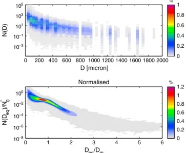
0 200 400 600 800 1000 1200 1400 1600 1800 2000 N(D) D [micron] % 0 0.2 0.4 0.6 0.8 1 Normalised D_eq/D_m 0 1 2 3 4 5 6 10−3 10−1 101 103 105 10−8 10−6 10−4 10−2 100 % 0 0.2 0.4 0.6 0.8 1 1.2 N(D eq )/N * 0

Figure 7. (a–k) Particle size distribution for different temperature ranges. These plots include all data. Grey line represents an exponential function.

that it is possible to have a slightly different behavior between Dmand N∗0distributions. We will come back

to these results later in section 6.2. Figure 7k shows the relationship between D_mand the temperature. Once again, the smallest values are observed for cold temperatures and the largest values are observed when we get closer to the freezing level. Another very interesting result is the increase in the variability around the mean value when temperatures get warmer. When temperatures increase, the range of diameters increases as we can have ice particles coming from different microphysical processes with an increasing role played by the aggregation process.

4.3. Impact of the Normalization on the Moments of the PSD

Cloud variables (IWC, visible extinction, and effective radius) and observed parameters can be expressed as moments of the PSD. We can therefore envisage expressing each moment as a function of Dmand N∗0.

Figure 8 shows the results of the normalization on the IWC, extinction, and reflectivity. Figure 8a exhibits IWC as a function of D_mand Figure 8b IWC divided by N∗

0in log space. This is an expected result as Dm,

IWC, and N∗

Figure 8. Impact of the normalization on different moments of the particle size distribution. (a, c, e, and g) IWC-D_m,

IWC-Z, IWC-extinction, andZ-extinction relationships, respectively. (b, d, f, and h) The result of the normalization for

each relationship.

the development of lookup tables linking the observations (Z,𝜎 from lidar backscatter) to cloud proper-ties which are used in many retrieval techniques. The normalization by N∗

0reduces the scatter as shown

by Figures 8b–8d, 8f, and 8h which represent IWC-Z, IWC/N∗ 0-Z/N ∗ 0, IWC-extinction, IWC/N ∗ 0-extinction/N ∗ 0, and Z-extinction, Z/N∗

0-extinction/N0∗relationships, respectively. In this situation, some of the variability is

incorporated in N∗

0and implies that it can be used a as common denominator for cloud and observed

vari-ables [Delanoë et al., 2007; Delanoë and Hogan, 2008]. As a result, using equation (12), it is possible to build lookup tables linking Dmto all normalized parameters (IWC/N∗0, extinction/N∗0, Z/N∗0). Note that reand Vtdo

not need to be normalized as they are independent of N∗

0. If we assume a single normalized PSD shape for

all ice clouds, it is therefore not necessary to fit the relationships between cloud variables. The main advan-tage in using the normalization approach versus a basic fit (between variables) is the resulting consistency in the relationship between different PSD moments. For instance, if we have two independent measurements (Z and visible extinction) and we want to retrieve the PSD, it is possible. IWC, Z, and the visible extinction are all linked by N∗

0and Dm. The remaining scatter obtained after normalization actually reflects the natural

variability of the normalized PSD shape and the assumption of a single M(D).

In order to use equation (12), it is necessary to obtain the best coefficients (𝛼 and 𝛽) to represent the normalized PSD. It is the aim of next section.

5. Best Parameterization for the Normalized PSD

5.1. Approach Used

Delanoë et al. [2005] showed that it was possible to represent the normalized PSD using the modified gamma function represented by equation (12). Several pairs of coefficients (𝛼 and 𝛽) were used to estimate the optimal representation. In this paper we use a slightly different approach; the optimal coefficients are derived using a least square regression linear fit on moments of the PSD as proposed by Field et al. [2005, 2007]. The main difference here is that we are using several combinations of moments to get the optimal

Table 4. Optimal Coefficients for the Modified Gamma for Each Campaigna

Moments Ext-Z Ext Z

Campaigns 𝛼_PSD 𝛽_PSD 𝛼_PSD 𝛽_PSD 𝛼_PSD 𝛽_PSD TC4 −0.113 1.765 −0.435 2.126 −0.193 1.798 NAMMA −0.391 1.737 −1.466 4.912 −0.189 1.645 CRYSTAL-FACE −0.442 1.557 −0.888 3.980 −1.765 2.518 ARM −0.085 2.100 −0.978 2.639 −0.059 2.168 M-PACE −1.948 8.798 −0.069 1.567 −2.187 12.477 C3VP 0.024 2.114 −1.122 8.620 8.817 0.599 AIRS −0.055 1.689 −1.386 8.216 −0.013 1.630 Subvisible −1.463 3.105 −1.899 6.600 −0.158 1.792 All −0.262 1.754 −1.254 4.189 −0.234 1.709 All (DARDAR) −0.237 1.839 −0.044 1.633 −0.189 1.827

a_{Extinction and/or reflectivity has been used to fit the theoretical shape.}

(𝛼, 𝛽) pair. For instance, we use a low moment of the PSD, the visible extinction, and the reflectivity factor a high moment of the PSD. The best coefficients,𝛼 and 𝛽, are obtained by minimizing the cost function J:

J = n ∑[( 1 −extnorm(𝛼, 𝛽) exttrue )2 + ( 1 −Znorm(𝛼, 𝛽) Ztrue )2] , (17)

where n is the number of component PSDs, ext_trueand Z_trueare the extinction and the reflectivity computed using the measured PSD, and extnormand Znormare derived using the normalized PSD. Note that we actually

minimize the ratio between the normalized PSD and the true PSD, aiming to avoid imbalance between the contribution of the two moments in the cost function. It is also possible to use only one of the moments for the minimization. Extinction and reflectivity are computed using the normalized PSD shape using the measured area and mass-size relationships Dmand N∗0derived from the measured PSD.

5.2. Coefficients of the Analytical Normalized PSD

The best analytical normalized PSD coefficients (𝛼 and 𝛽) are summarized in Table 4, using extinction and/or reflectivity as noted above.

Figure 9 illustrates the results in terms of PSD shape for each campaign and for all campaigns combined. Figures 9a–9c represent the parameterized PSD when extinction and/or reflectivity is used in the mini-mization process, respectively. Figure 9d shows𝛽 coefficients as a function of 𝛼 coefficients. Except for the M-PACE campaign (using extinction-Z couple and Z only), the shapes are very similar in the range 0.5 < D_eq∕D_m< 1.5 where the data are concentrated. This result is consistent with Figure 4, and differences are observed for the wings of the distribution. However, it is obvious that the choice of the moment to fit the PSD is crucial. A low-order moment is mainly weighted by the small particles while a high-order moment is weighted by large particles. For this reason the ability of the normalized PSD to represent small or large par-ticles depends on the pair of coefficients. This is why we suggest using visible extinction and reflectivity to derive those coefficients.

The tail of the distribution is strongly constrained by the reflectivity while the shape of the distribution for small normalized diameters is driven the extinction. When normalizing the PSD, this relationship is not as straightforward, as small and large particles are spanning the whole Deq∕Dmrange.

5.3. Impact of the Normalized Coefficient on the Cloud Variables and the Radar Measurements

In the previous section, we saw the impact of the derived coefficients on the normalized PSD shape. In this section we show the impact of the normalized PSD shape on cloud and observed variables. Therefore, visible extinction, effective radius, reflectivity, and terminal fall velocity are computed using the observed PSD and the derived mass-size relationships and they are compared to those obtained using the analytical shape and the retrieved𝛼 and 𝛽. It is important to note that we do not have to evaluate the impact of the normalized PSD on IWC as it is directly computed from N∗

0 1 2 3 4 10−6 10−4 10−2 100 D_eq/D_m N(D eq )/N 0 * 0 1 2 3 4 10−6 10−4 10−2 100 D_eq/D_m N(D eq )/N 0 * 0 1 2 3 4 10−6 10−4 10−2 100 D_eq/D_m N(D eq )/N 0 * Ext and Z

a)

Ext

b)

Z

c)

TC4 CF NAMMA ARM M−PACE AIRS C3VP SUBVIS All −5 0 5 10 0 2 4 6 8 10 12 14 α β

d)

ext−Z ext Z

Figure 9. Idealized representation of the normalized PSD (modified gamma shape) for each data set, obtained after minimization using (a) extinction and reflectivity, (b) extinction alone, and (c) reflectivity factor alone. Coefficients of the modified gamma shapes can be found in Table 4 and are represented in panel (d).

Figure 10 summarizes the relative mean difference and the standard deviation between the measured PSD and the analytical shape. The full description of Figure 10 is given in the caption. The mass-size relationships, used for the calculations, have been retrieved using the PSD and the direct measurements of IWC. The cor-responding M(D) will be referred to as the “retrieved” M(D). Note that we actually compare the normalized parameters (i.e., independent of N∗

0) but this is strictly equivalent to comparing the unnormalized

parame-ters as N∗

0cancels out when we compute the ratio. The pairs of coefficients used for computing the analytical

PSD are those presented in the previous section and summarized in Table 4. The most important result here is that the pair of coefficients derived using the full data set gives very similar results to the pairs of coeffi-cients derived for each campaign. The bottom panel also shows the distribution of each cloud variable or radar measurement (extinction, effective radius, radar reflectivity, and terminal fall velocity), which indicates where it is most important to have the smallest differences.

1. The relative mean difference for visible extinction (Figures 10a, 10e, and 10j) is between −10% and 10% where most of the data are concentrated, i.e., where visible extinction is greater than 1 e−5_m−1

(Figure 10n). This is verified independently on the constraint (i.e., Z only, Z and extinction, or extinction only), which is used to retrieve the pair of coefficients. As expected, for the small extinction values (i.e., less than 5 e−4 _m−1_{), the lowest relative mean difference for extinction is obtained when visible}

extinc-tion is used as a constraint to fit the analytical PSD shape. In this configuraextinc-tion, we observed the lowest difference variability; the envelope (i.e., ± standard deviation) belongs to the [−15%, 15%] interval. The envelope shown for the full data set pair of coefficients (red one) is narrower than for the “campaign” pair of coefficients (black one) when Z is used as the only constraint (Figure 10j). This is not surprising due to the difference in the order of the moments. However, the relative mean difference is slightly closer to zero for large extinctions (larger than 5 e−4_m−1_{) when Z is the only constraint.}

2. The relative mean difference for r_e(Figures 10b, 10f, and 10k) is consistent with the relative mean differ-ence for visible extinction with values within the [−10% 10%] range. This is an expected result as reis a

combination of IWC and visible extinction (equation (16)) and IWC∕N∗

Figure 10. Relative mean difference (in percent) between (a, e, and j) extinction, (b, f, and k)r_e, (c, g, and l)Z, and (d, h, and m)V_tcomputed with the analytical

gamma shape and the measured PSD.𝛼and𝛽coefficients which are used to compute cloud and observed variables are obtained using different constraints

(Figures 10a–10d:Zand extinction; Figures 10e–10h: only extinction; Figures 10j–10m: onlyZ). Black lines represent variables retrieved using the best𝛼and𝛽

coefficients for each campaign while red lines correspond to variables computed with coefficients derived from the full data set. Thickest lines are the mean

values and thinnest lines represent the envelopes (mean±standard deviation.) Figures 10n–10q illustrate the number of data points used to compute the mean

values. The retrievedM(D)is assumed.

3. Figures 10c and 10l show that the relative mean difference for Z is around −10% when Z is used as constraint. This difference seems to be smaller if extinction is used (Figure 10g), within average less than a few percent. However, the absolute relative mean difference strongly increases for large val-ues of reflectivity, i.e., Z> 10dBZ. The relative standard deviations are about 15%–20% for the three presented configurations.

4. The absolute relative mean difference for Vt(reflectivity weighted terminal fall velocity) exhibits different

results compared to other variables. When Vtis less than 0.5 m s−1, it can exceed 20% if we use a pair of

coefficients derived using Z. It does not exceed 10% when Vt> 0.7 m s−1.

We can conclude that for the visible extinction, r_e, Z, and V_t, the absolute relative mean difference is approximatively 10% if we use the full data set𝛼 and 𝛽 coefficients. These results are consistent with Delanoë et al. [2005].

5.4. Impact of the Mass-Size Relationship on the Normalized PSD

In satellite retrieval techniques, it is common to use a single mass-size relationship (or a combination) as it remains difficult to adjust M(D) due to a lack of independent measurements. Our objective in this section is to assess whether the mass-size relationship choice is crucial in the characterization of the analytical normalized PSD. We also propose to quantify the error made if we use a more commonly used mass-size relationship instead of the retrieved M(D) in the cloud and observed variables computed using the analytical normalized PSD shape.

Figure 11. Same as Figure 10 but DARDARM(D)is assumed. See text for details or color significations.

The first step is to retrieve𝛼 and 𝛽 coefficients with the same mass-size assumption as the DARDAR prod-uct (see section 3.3). Those coefficients can be found in Table 4 and are referred to as DARDAR. Figure 11 is the same as Figure 10, where red color is attributed to the relative mean difference (and standard deviation) between cloud and observed variables computed with the analytical normalized PSD and the observed PSD assuming DARDAR M(D). Black lines are the relative mean difference (and standard deviation) between cloud and observed variables computed with the analytical normalized PSD assuming DARDAR M(D) and the observed PSD using the retrieved M(D). In the next section, it will be referred as the relative mean differ-ence between the DARDAR and the observed PSD. From this figure we can conclude that the impact of the choice of M(D) is very large compared to the choice of𝛼 and 𝛽 coefficients. This is a strong result regarding the normalization approach.

As shown in Figures 11a–11m, the error (including bias and variability) due to the use of the normalized approach, when we assume the same mass-size relationship (red curves), is considerably smaller than the error due the M(D) assumption (black curves). This statement is valid for both cloud (extinction, effective radius) and measurement parameters (V_t, Z). We also see that relative mean difference and relative standard deviation values strongly vary with the assessed variable range, for instance the relative mean difference in Zgoes from −50% for reflectivity below −40 dBZ to 95% for high reflectivity (Figures 11c, 11g, and 11i).

6. Parameterization for Key Ice Cloud Parameters

We demonstrated the impact of using the normalized PSD and showed that it could be represented by an analytical function. As a result, if we can retrieve N∗

0and Dm, it is therefore possible to approximate the

par-ticle size distribution (N(Deq) = N∗0F𝛼,𝛽(Deq∕Dm)). However, one of the two moments is sometimes missing

Figure 12. A priori values forN∗

0andN′0. (a)N∗0computed using measured PSD and retrievedM(D)as a function of

tem-perature. The black line is the corresponding parameterization. (b)N′

0as a function of temperature. The red lines are the

parameterizations for DARDARM(D). (c, d) RetrievedN∗

0, usingN∗0andN′0temperature parameterizations (retrievedM(D)

only), respectively. Color contours show the number of data in Figures 12a–12d.

lidar-only retrievals for instance, where only one constraint is available and a parameterization of one of those two scaling parameters is needed). Some moments of the PSD, such as Vt, do not depend on N∗0, and

consequently, we will retrieve D_musing the radar Doppler velocity [Delanoë et al., 2005, 2007]. Therefore, in the next section we investigate different possible options to parameterize N∗

0using either temperature

or D_m.

6.1. An A Priori for N∗₀and N′₀

Delanoë and Hogan [2008] showed that there was a clear temperature dependence of N∗

0but that the

derived relationship was strongly dependent on the IWC. Note that in this previous study, bulk measure-ments of IWC were not available and the mass-size relationship used was that from Brown and Francis [1995]. Figure 12a shows the relationship between N∗

0and temperature using the retrieved M(D) and the measured

PSD. The black line represents the corresponding parameterization and is expressed as ln(N∗ 0) = A1N∗ 0T + A2N∗0, (18) where A1N∗ 0and A2N ∗

0coefficients can be found in Table 5, T is the temperature in degrees Celsius, and N

∗ 0

is in m−4_{. The red line illustrates the relationship obtained if we use the measured PSD and the DARDAR}

mass-size relationship. The coefficients A_1N∗

0and A2N∗0corresponding are also presented in Table 5. Both

rela-tionships are very similar; this is an expected result as the DARDAR N∗

0is on average 1.4 time N∗0with the

measured M(D). Therefore, the change appears very small in log space. Figure 12c compares N∗

0obtained from the measured PSD (x axis) against the one computed using the

parameterization (y axis). We can see that the parameterization does not capture the variability of N∗ 0. The

retrieved values are confined between about 108_{and 10}10_m−4_{. The difficulty in representing the extreme}

Table 5.N∗

0(T) andN′0(T) Parameterization Coefficients

N∗

0(T) N′0(T)

Mass-Size Relationship A_1N∗

0 A2N∗0 n A1N′0 A2N′0

Retrieved relationships [Heymsfield et al., 2010] −0.081014 17.469 1.1 −0.10757 24.9

values of N∗

0can be a problem for establishing our a priori information. As a result, Delanoë and Hogan [2008]

proposed to use a new variable N′

0which depends on N∗0and visible extinction: N′

0= N ∗ 0∕𝜎

n_{. (19)}

where𝜎 is the visible extinction per meter and n a coefficient which can be adjusted. This choice was driven by the idea of using a variable which is very well constrained by the lidar measurement.

The parameterization as a function of temperature is the following: ln(N∗

0∕𝜎

n_{) = A}

1N′

0T + A2N0′ (20)

where T is the temperature in degrees Celsius and A_1N′

0, A2N0′, and n are in Table 5. By minimizing the least

square sense the difference between N∗

0and the retrieved values using equation (20), n, A1N′

0, and A2N′0

are obtained.

Figure 12b represents the N′

0variable as a function of temperature using n = 1.1. Both parameterizations

using measured M(D) and DARDAR are plotted on the contour representation. As it was the case for coef-ficients A_1N∗

0and A2N∗0, A1N0′and A2N0′coefficients are similar for the retrieved M(D) and DARDAR. Note that

extinction which is used to derive the relationships is directly computed from area dimensional probes mea-surements. As shown in Table 5, n coefficients for the retrieved M(D) and DARDAR are very close to 1. This result implies that the𝜎∕N∗

0ratio would also be a good candidate for the a priori information. The slight

dif-ference is certainly due to the fact that we use an extinction directly derived from the probes and not from a simple parameterization. However, the n coefficient differs from the one proposed in Delanoë and Hogan [2008] (n = 0.6). This is due to the choice of the mass-size and area-size relationships assumed to calculate extinction and the moments of the PSD.

Figure 12d illustrates the result of applying the parameterization obtained for the measured M(D). We clearly see that dividing N∗

0by a power of extinction allows us to derive a parameterization valid for whole range

of N∗

0. This is a striking result compared to the simple N ∗

0(T) parameterization. An error assessment, not

shown here, has been carried out and showed that for both parameterizations the mean relative error on N∗ 0

exceeds 200%. As N∗

0is not a real cloud variable, we propose to evaluate the error of both parameterizations

on IWC. To do so we first derive a parameterization of IWC as a function of N∗

0and Z and then use the N ∗ 0(T) and N′ 0(T) to calculate N ∗ 0.

Figure 13 is a contour plot of the IWC∕N∗

0as a function of Z∕N ∗

0. As mentioned in section 4.3, the impact of

the normalization is obvious. We can distinguish two areas. The first one shows a linear variation between the logarithm of IWC∕N∗

0and Z∕N ∗

0, which corresponds to the Rayleigh regime region (particle size is small

enough with respect to the radar wavelength) when_NZ∗ 0 ≤ 10

−10_mm6_{m. The second area, when} Z N∗

0 > 10

−10

mm6_{mshows the Mie effects and the reflectivity cannot be approximated by the sixth moment of the}

PSD anymore. Taking this into account, we derive, depending on the Rayleigh/Mie regime, two different parameterizations: when_NZ∗ 0 ≤ 10 −10_mm6_m log10 ( IWC N∗ 0 ) = 0.5787 log₁₀ ( Z N∗ 0 ) − 4.8923 (21) and when Z N∗ 0 > 10 −10_mm6_m log10 ( IWC N∗ 0 ) = 0.0258 log₁₀ ( Z N∗ 0 )3 + 0.7629 log₁₀ ( Z N∗ 0 )2 + 8.1496 log₁₀ ( Z N∗ 0 ) + 20.3024 (22) where Z is in mm6_m−3_{, N}∗ 0in m−4, and IWC in g m−3.

The two relationships are represented by the red curve in Figure 13. Note that we constrained the relation-ships in a way that we avoid any discontinuity between the two regimes. In Figure 14 we present the impact of using N∗ 0(T) or N ′ 0(T) in the IWC/N ∗ 0- Z∕N ∗

0relationship. Figure 14a corresponds to a scatterplot between

the measured IWC and the parameterized IWC using N∗

Figure 13. Relationship between normalized IWC andZin log space. The filled contours show the number of points. The red curve represents a parameterization of the relationship, combining a linear function for the Rayleigh regime part and cubic function when the Rayleigh approximation is not applicable. The relationships are given in the text.

but for N′

0(T) parameterization. For the latter we have used the measured extinction. Note that this

extinc-tion could be provided by lidar measurements in a retrieval technique context. From these two panels, we can see that the N′

0(T) parameterization gives better results and the scatterplot is closer to the 1:1 line

than the N∗

0(T) relationship. This result is confirmed by Figure 14c. It shows the mean relative difference

between the retrieved IWC and the measured IWC as a function of the measured IWC. For large IWC (i.e., IWC > 0.01 g m−3_{), the N}∗

0(T) relationship gives good results with a mean relative difference within the range

Figure 14. Impact of theN∗

0(T)andN′0(T)relationships on the retrieval of IWC using the IWC/N∗0-Z∕N∗0relationship

pre-sented in Figure 13. (a, b) Scatterplots of parameterized IWC versus measured IWC. (c) The mean relative difference (thick

lines) and its envelope (thin lines) between measured and parameterized IWC: black lines for theN∗

0(T)and red lines

forN′

Figure 15.N∗

0-Dmrelationships. (a) A PDF ofN∗0(m−4) as a function ofDm(micron) computed using the measured PSD

and retrievedM(D). Black lines representN∗

0-Dmrelationships at constant IWC. (b) Identical to Figure 15a but including

fits for each temperature range. (c) The same as Figure 15b assuming DARDARM(D). (d) Parameterizations obtained

for the full range of temperature for the retrieved and DARDARM(D)are compared. Isocontours represent the number

of data.

−10% +10% while the N′

0(T) parameterization show a larger mean relative difference from −60% to 20%. If

the first one produces the smallest differences for large IWC, it cannot be used for IWC< 0.001 g m−3_{) as the}

absolute mean relative difference exceeds 300%. The N′

0(T) relationship is satisfactory as it produces an absolute mean difference smaller than 80% over the

whole range. It is therefore obvious that the N′

0(T) relationship is much more appropriate than the simple N∗

0(T) parameterization; however, the extinction knowledge is required.

6.2. N∗

0-DmRelationship

Figures 15a to 15c represent the PDF (probability distribution function) of N∗

0as a function of Dm. N∗0and Dm

are computed using the measured PSD and the retrieved M(D) or DARDAR M(D). As noted earlier there is an analytical relationship between D_mand N∗

0, and this relationship depends on IWC. These relationships are

presented in Figure 15a, where each black line corresponds to a constant value of IWC. Contours show that most of the data are spanning 10−4_{g m}−3_{and 1 g m}−3_{. It is also shown that the shape of the relationship is}

totally described by IWC. Unfortunately, in most cloud retrieval methods, IWC is unknown. Therefore, we are looking for a relationship between Dmand N∗0which can be expressed as follows:

N∗ 0= KD

L

m, (23)

where K and L, reported in Table 6, are the best coefficients obtained by fitting the relationship between N∗

0and Dmin log space. They are computed for both M(D), and the results are overplotted as a black or red

dotted line. These coefficients can be computed for different ranges of temperature. Solid colored lines rep-resent the parameterizations obtained for 10◦C temperature intervals ranging from −6 to −56◦C. These results illustrate that temperature affects the N∗

0-Dmrelationship, with a jump near −36◦C. Because small Dm

and high N∗

0correspond to cold temperatures, the fit is calculated on a much smaller range of values and the

representation of Dmabove 400μm (cf. 7i) should not be taken into account.

Figure 15d presents the PDF as isocontours, with parameterizations derived for retrieved M(D) and DARDAR M(D). The change in the choice of the mass-size relationship does not affect the relationship between N∗

0

and Dm.

Table 6.N∗

0-DmParameterization Coefficients

Mass-Size Relationship K L

Derived relationships [Heymsfield et al., 2010] 1.07e14 −2.19

DARDAR 5.65e14 −2.57

The main effect is to contract or dilate the N∗

0and Dmranges without

signifi-cantly changing the parameterization. This is clearly an advantage and it is then possible to use the relationship between N∗

that the idea is not to propose a very accurate parameterization and this is why we do not evaluate the error produced by using that parameterization. We show that it is possible to use this relationship to constrain a variational algorithm for instance by ensuring that the retrieved values belong to the envelope described by the contours [Delanoë and Hogan, 2008].

7. Summary and Discussion

The aim of the paper was to update the Delanoë et al. [2005] study on the normalized PSD approach. The main improvement resided in the use of a very large in situ data set including bulk measurements of the IWC. It also included direct measurements of the projected areas of the ice particles which allowed to com-pute a good proxy of visible extinction and could be combined with M(D) to derive a realistic terminal fall velocity [Heymsfield and Westbrook, 2010]. We also proposed an optimized approach to derive the coeffi-cients of the modified gamma representing the normalized PSD. A combination of two key measurement moments was presented for retrieving the coefficients. Once the coefficients are retrieved, we analyzed the impact of using the normalized approach for computing cloud and measurement variables. The impact of the temperature on the normalized PSD shape has been addressed in section 4.2. However, we have tried to parameterize the PSD shape as a function of temperature but the results were not conclusive and for this reason it was not presented in the study.

In section 5.4, the impact of M(D) on the PSD shape retrieval was assessed. It was shown that the choice of the mass-size relationship did not change the conclusions regarding the benefit of the normalization approach. It was also obvious that the error in selecting the M(D) was much larger than a wrong choice of the normalized modified gamma coefficients. This was not a surprise as it was clearly stated that most of errors come from M(D) in cloud retrievals [Heymsfield et al., 2010]. It could be envisioned to implement the normalized approach in the nonhydrostatic mesoscale atmospheric model of the French research commu-nity (Meso-NH) mesoscale model [Lascaux et al., 2006]. A similar approach, using Field et al. [2007], has been introduced operationally on 17 January 2012 (PS28) in the UKMO global-scale model. The benefit would be the use of a single gamma shape representation for the different ice hydrometeor classes.

Appendix A: Impact of Small Particles on the PSD Shape

A1. Shattering Effect

As mentioned in section 3.2, the data used in this study are corrected from the shattering effect using par-ticle interarrival times. The shattering effect can contaminate the number concentration of parpar-ticles by artificially increasing the number of small particles which originates from the breakup of larger ice crys-tals on the probe’s inlet. In this section, we examine the impact of the shattering correction on the results, by repeating the results presented in sections 4 and 5 but without the correction using particle interarrival times. We also introduce a shattering parameter, which varies between 0 and 1 and indicates the propor-tion of particles which have naturally occurring interarrival times as identified by the correcpropor-tion algorithm using Poisson counting statistics. Note that we consider a low-shattering environment to exist when this parameter is above 0.8. The impact of the shattering correction on the normalized PSD shape is presented in Figure A1. Figures A1a–A1c represent the normalized PSD when the particle concentration is not cor-rected from shattering, when it is corcor-rected, and when only low-shattering environments are considered, respectively. The distribution of shattering parameter is shown in Figure A1f, and less than 23% of data are below the shattering parameter threshold. The contour plots (Figures A1a–A1c) show very similar pat-terns; however, the uncorrected normalized PSD distribution indicates a higher data concentration below Deq∕Dm = 0.5 than the corrected data. This is an expected result as the concentration of small particles is

higher. When the data which are potentially prone to shattering contamination are removed, we observe even less data in the Deq∕Dm < 0.5 area. Figures A1d and A1e are idealized representations of the

normal-ized PSD (modified gamma shape) for the corrected (black lines), uncorrected (red lines), and corrected with low-shattering environment (blue lines). The gamma modified (𝛼, 𝛽) coefficients are derived using extinction and reflectivity (Figure A1d) or extinction only (Figure A1e). When (𝛼, 𝛽) pair is derived using extinction and reflectivity, we can see that there are almost no changes in the results. However, we observe a difference in the results when we use only extinction to derive the (𝛼, 𝛽) coefficients. The red and black curves are in very good agreement, but the shape corresponding to the “low-shattering” data is different when Deq∕Dm> 2.

Figure A1. Impact of the shattering correction on the normalized PSD shape. The calculations involved PSD corrected and uncorrected from the shattering effects and also the corrected PSD when we have a low-shattering environment (see details in the text). (a–c) The normalized PSD. (d, e) Idealized representations of the

normalized PSD. (f ) The distribution of shattering parameter. Relative mean difference (in percent) between (g, j) extinction, (h, k)Z, and (i, l)Vtcomputed with

the analytical gamma shape and the measured (corrected and uncorrected) PSD. Color codes are described in the text.

mean differences (in percent) between extinction for Figures A1g and A1j, Z for Figures A1h and A1k, and Vt

for Figures A1i and A1l computed with the analytical gamma shape and the measured (corrected or uncor-rected) PSD. Solid lines are the relative mean differences and the dashed lines are the ±1 standard deviation. For these six panels, the color codes are the following:

1. Black lines - PSD coefficients are derived using the corrected PSD, and the reference (normalized extinction, normalized reflectivity, and terminal fall velocity) is the corrected PSD.

2. Red lines - PSD coefficients are derived using the uncorrected PSD, and the reference is the corrected PSD. 3. Blue lines - PSD coefficients are derived using the corrected and shattering coefficient greater than 0.8

PSD, and the reference is the corrected PSD.

4. Green lines - PSD coefficients are derived using the corrected PSD, and the reference is the uncorrected PSD.

5. Magenta lines - PSD coefficients are derived using the corrected and shattering coefficient greater than 0.8 PSD, and the reference is the uncorrected PSD.

We can consider that the impact of using the uncorrected, corrected, or shattering coefficient greater than 0.8 is not large when the coefficients are derived using extinction and reflectivity (Figures A1g–A1i). This is due to the fact that the reflectivity is not sensitive to small particles and counterbalances the impact on the extinction. We can use the coefficients derived using the corrected (with or without threshold on the shattering parameter) or uncorrected PSD to represent the normalized PSD if we are using radar and lidar measurements. However, the results are slightly different when only extinction is used to derived the nor-malized PSD coefficients. The change in the coefficients introduces biases in the retrieved Z (10% below −10 dBZ) and V_t(10% below 1.2 m s−1_{). Note that the standard deviations are within the same range}

inde-pendently of the PSD used. Despite small changes in the PSD shape, we show that the presence of shattered particles does not change the main results of the study. Note that the data used in the main study are corrected from the shattering effects.