HAL Id: hal-00923340
https://hal.archives-ouvertes.fr/hal-00923340
Submitted on 12 Jan 2017
HAL is a multi-disciplinary open access
archive for the deposit and dissemination of sci-entific research documents, whether they are pub-lished or not. The documents may come from teaching and research institutions in France or abroad, or from public or private research centers.
L’archive ouverte pluridisciplinaire HAL, est destinée au dépôt et à la diffusion de documents scientifiques de niveau recherche, publiés ou non, émanant des établissements d’enseignement et de recherche français ou étrangers, des laboratoires publics ou privés.
interfaces: analysis with the small perturbation method
and the small slope approximation
A. Berrouk, Richard Dusséaux, Saddek Afifi
To cite this version:
A. Berrouk, Richard Dusséaux, Saddek Afifi. Electromagnetic wave scattering from rough layered interfaces: analysis with the small perturbation method and the small slope approximation. Progress In Electromagnetics Research B, EMW Publishing, 2014, 57, pp.177-180. �10.2528/PIERB13101802�. �hal-00923340�
Electromagnetic Wave Scattering from Rough Layered Interfaces:
Analysis with the Small Perturbation Method and the Small
Slope Approximation
Abla Berrouk1, Richard Duss´eaux2, *, and Saddek Afifi3
Abstract—We propose a theoretical study on the electromagnetic wave scattering from layered structures with an arbitrary number of rough interfaces by using the small perturbation method and the small slope approximation. The interfaces are characterized by Gaussian height distributions with zero mean values and Gaussian correlation functions. They can be correlated or not. The electromagnetic field in each medium is represented by a Rayleigh expansion and a perturbation method is used for solving the boundary value problem and determining the first-order scattering amplitudes by recurrence relations. The scattering amplitude under the first-order small slope approximation are deduced from results derived from the first-order small perturbation method. Comparison between these two analytical models and a numerical method based on the combination of scattering matrices is presented.
1. INTRODUCTION
The study of electromagnetic wave scattering from rough layered interfaces has many applications in remote sensing, communication techniques, civil engineering, geophysics and optics. Several models give the average scattered field and the average intensity. Analytical methods are based on physical approximations and give closed-form formulae for the first- and second-order moments of the scattered field. Exact methods estimate the average scattered field and the average intensity from the results over many realizations of rough layered interfaces. In this paper, we propose a theoretical study on the electromagnetic wave scattering from layered structures with an arbitrary number of rough interfaces by using two analytical models: the first-order small perturbation method (SPM) and the first-order small slope approximation (SSA).
Elson was one of the first authors to develop a vector theory of scattering from a stratified medium. This vector theory allows the angular distribution of scattered light to be determined and can be used with correlated or uncorrelated surface roughness [1, 2]. The SPM has been used for the study of light scattering from multilayer optical coatings [1–5] and many authors have also implemented a perturbative theory for analyzing remote sensing problems [6–12]. The small slope approximation (SSA1) has an extended domain of applicability [13–15] which includes the domain of the small-perturbation method that is only valid for surfaces with small roughness [16] and the domain of the Kirchhoff approximation that is applicable to surfaces with long correlation length [17, 18].
In the present paper, the structure under consideration is a stack of several rough one-dimensional interfaces. The interfaces are characterized by Gaussian height distributions with zero mean values and Gaussian correlation functions. The electromagnetic field in each region is represented by a continuous spectrum of plane waves, the amplitudes of which are found by matching the boundary conditions
Received 18 October 2013, Accepted 25 November 2013, Scheduled 6 December 2013
* Corresponding author: Richard Duss´eaux ([email protected]).
1 Laboratoire d’´Etude et de Recherche en Instrumentation et en Communication d’Annaba (LERICA), Badji Mokhtar-Annaba
University, Annaba 23000, Algeria. 2 Universit´e de Versailles Saint-Quentin en Yvelines, LATMOS/IPSL/CNRS, 11 Boulevard
d’Alembert, Guyancourt 78280, France. 3 Laboratoire de Physique des Lasers, de Spectroscopie Optique et d’Opto-´electronique
for both interfaces. The boundary value problem is imposed up to the first-order and the scattering amplitudes are derived from recurrence relations [6]. The scattering amplitudes under the first-order small slope approximation are deduced from results derived from the first-order small perturbation method. We establish the closed-form formulae for the coherent and incoherent intensities of the electromagnetic wave scattering from layered structures. In [14], the authors extended the SSA to the fourth-order terms of the perturbative development and studied a slab with uncorrelated rough two-dimensional interfaces. In the present paper, we consider the first-order SSA method applied to an arbitrary number of one-dimensional interfaces. Moreover, the interfaces can be uncorrelated, partially or fully correlated. To our knowledge, this is a novelty. We also compare these two methods with each other and with a Rayleigh-Fourier method extended to multilayer structures and based on the combination of elementary scattering matrices of different interfaces [19, 20].
2. STATISTICAL DESCRIPTION OF INTERFACES
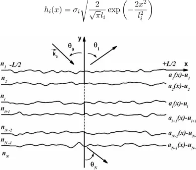
The geometry of the structure is described in Figure 1. We consider a stack of several rough one-dimensional interfaces. These surfaces are randomly deformed over a length L. For the study with both analytical models, L will be extended to infinity. Both interfaces i and i + 1 are separated by a layer with thickness di = ui+1− ui (with u1 = 0). N designates the number of media.
Each interface is a Gaussian random process, centered (hai(x)i = 0, ∀x) and stationary to the
second order. Henceforth, the angular brackets h i stand for statistical averages. The random interfaces are uncorrelated, partially or fully correlated. We denote Rii(x) the autocorrelation function associated
with the interface i and Rij(x), the cross-correlation function between the interfaces i and j. The
random functions ai(x) are obtained by filtering of uncorrelated white noises bj(x):
ai(x) = hi(x) ∗ N −1X j=1 pijbj(x) (1) where N −1X j=1 p2ij = 1 (2)
The symbol ∗ designates the convolution operation. The functions hi(x) are the impulse responses of Gaussian filters defined by:
hi(x) = σi s 2 √ πliexp µ −2x2 l2 i ¶ (3)
The autocorrelation (i = j) and cross-correlation (i 6= j) functions are expressed as follows: Rij(x) = ai(x0)aj(x + x0) ® = qij +∞ Z −∞ hi(x0)hj(x + x0)dx0 (4) where qij = N −1X k=1 pikpjk (5) According to (3), we have: Rij(x) = qijσiσj s 2lilj l2 i + l2j exp à − 2x2 l2 i + lj2 ! (6)
σi is the rms height of the interface i and li the correlation length. If qi,j6=i = 0, the interfaces i and
j are uncorrelated. They are fully correlated for li = lj and qij = ±1. They are partially correlated
in other cases. According to (6), the roughness spectra of interfaces (i = j) and their cross-spectral density (i 6= j) are given by:
ˆ Rij(α) = FT [Rij(x)] = +∞ Z −∞ Rij(x) exp(+jαx)dx = qijσiσj p πliljexp " −α2(l 2 i + l2j) 8 # (7) Thereafter, the letters FT designate the Fourier Transform operation.
3. INCIDENT FIELD AND SCATTERED FIELDS
The structure is illuminated by a monochromatic plane wave with a wavelength λ and a harmonic temporal dependence exp(jωt). The incident wave vector ~k0 is located in the xOy plane and forms
the angle θ0 with the Oy axis. Medium 1 is assimilated to the vacuum. Z is the vacuum impedance
and k = 2π/λ, the wave number. Henceforth, εri, ni, Zi and ki designate the relative permittivity, the
optical index (ni =√εri), the impedance (Zi = Z/ni) and the wave number (ki = nik) of the layer i.
Let F0(x, y) the Oz-component of the incident field of amplitude A0:
F0(x, y) = A0exp [−j (α0x − β0y)] (8)
α0 and β0 are the propagation coefficients with α2
0+ β02 = k2. For the polarization E//, the electric field
vector is parallel to the Oz axis and F0(x, y) = E0z(x, y). For the polarization H//, it is the magnetic field vector which is parallel to the Oz axis and F0(x, y) = Z1H0z(x, y).
In each medium, the scattered field is represented by a continuous spectrum of plane waves, commonly called Rayleigh expansion. In medium 1, the Oz-component is given as follows:
F1(x, y) = 2π1
Z +∞
−∞
A1(α) exp [−j (αx + β1y)] dα (9)
In medium i with 2 ≤ i ≤ N − 1, it is necessary to consider upwards and downwards propagating waves.
Fi(x, y) = 2π1 Z +∞ −∞ A(−)i (α) exp [−j (αx − βiy)] dα + 1 2π Z +∞ −∞ A(+)i (α) exp [−j (αx + βiy)] dα (10)
In the lower medium N , the Rayleigh expansion is represented by downwards propagating waves:
FN(x, y) = 1 2π
Z +∞
−∞
Each plane wave is characterized by its wave function exp(−j(αx ± βiy)) and its wave vector ~k(∓)i =
α~ux∓βi~uy. The scattering amplitudes A(∓)i (α) represent the unknowns of the problem. The propagation
coefficients βi(1 ≤ i ≤ N ) present a negative or zero imaginary part with βi2+α2 = k2i. The propagation
coefficients βi associated with α0 are denoted βi0 = βi(α0). The magnetic components in polarization
E// and the electric components in polarization H// are deduced from the orthogonality relations between the electric vector, the magnetic vector and the wave vector of the elementary plane waves of the Rayleigh integrals defined by (9)–(11).
The normalized bistatic scattering coefficient is defined by the power scattered per unit angle divided by the flux of incident power through the modulated region of length L. In the upper medium, we have [16]:
I(θ) = |A1(α = k sin θ)|
2cos2θ
λ cos θ0L |A0|2 (12)
In the case of scattering from randomly rough interfaces, A1(k sin θ) is a random function of the
observation angle θ. We can write this function as a sum of an average amplitude hA1i and a
fluctuating amplitude defined by A1− hA1i. The average amplitude gives the coherent intensity IC(θ)
by substituting A1 by hA1i into (12) and the fluctuating amplitude gives the incoherent intensity with
If(θ) = hI(θ)i − IC(θ). hI(θ)i represents the bi-static scattering coefficient. Within the framework
of the small perturbation method and the small slope approximation, we consider interfaces with an infinite extension and we define the coherent and incoherent intensities from analytical calculations. With a numerical method, the intensities are estimated over results of several interface realizations of finite extension.
4. THE SMALL PERTURBATION METHOD (SPM)
4.1. The Rayleigh Hypothesis and the Boundary Condition Problem
The Rayleigh hypothesis is compatible with the Rayleigh expansion at any point of the space including the interfaces [21–24]. This hypothesis makes it possible to write the boundary conditions which stipulate the continuity of the electric and magnetic components parallel to the interfaces. The scattering amplitudes A(∓)i (α) satisfy the following equations:
ei[Fi(x, y)]y=ai(x)−ui = [Fi+1(x, y)]y=ai(x)−ui (13)
· ∂Fi(x, y) ∂y − ˙ai(x) ∂Fi(x, y) ∂x ¸ y=ai(x)−ui = ei · ∂Fi+1(x, y) ∂y − ˙ai(x) ∂Fi+1(x, y) ∂x ¸ y=ai(x)−ui (14) where ei = ½ 1 in E// ni/ni+1 in H// (15)
We determine the scattering amplitudes A1(α), A(±)i (α) and AN(α) within the framework of the first-order small perturbation method applied to the boundary value problem (13)–(14). The perturbation method consists in representing the scattering amplitudes and the elementary wave functions by expansions in entire series [1].
4.2. Zeroth- and First-order Small Perturbation Method
The zeroth-order problem gives the field scattered by a stack of perfectly smooth interfaces [1, 2, 25]. The zeroth-order boundary value problem on the interface i leads to the following matrix system,
" A(+,0)i (α0) A(−,0)i (α0) # = C(i,i+1)(α0) " A(+,0)i+1 (α0) A(−,0)i+1 (α0) # (16)
where for the polarization E//, the matrix C(i,i+1)(α) (here at the value α = α0) is given by C(i,i+1)E//(α) = βi+ βi+1 2βi exp[+j (βi+1−βi) ui] βi− βi+1 2βi exp[−j (βi+1+βi) ui] βi− βi+1 2βi exp[+j (βi+1+βi) ui] βi+βi+1 2βi exp[−j (βi+1−βi) ui] (17)
and for the polarization H//, by
C(i,i+1)H //(α) = n2 i+1βi+n2iβi+1
2nini+1βi exp[+j(βi+1−βi)ui]
n2
i+1βi−n2iβi+1
2nini+1βi exp[−j(βi+1+βi)ui]
n2
i+1βi−n2iβi+1
2nini+1βi exp[+j(βi+1+βi)ui]
n2
i+1βi+n2iβi+1
2nini+1βi exp[−j(βi+1−βi)ui]
(18) The product M1,N(α0) of N − 1 matrices C(i,i+1)(α0) yields the overall transfer matrix from medium
N to medium 1. · A(0)1 (α0) A0(α0) ¸ =M1,N(α) " 0 A(0)N (α0) # = " M1,N(+,+)(α0) M1,N(+,−)(α0) M1,N(−,+)(α0) M1,N(−,−)(α0) # " 0 A(0)N (α0) # (19) where M1,N(α0) = N −1Y i=1 C(i,i+1)(α0) (20)
We find from (19) the reflection coefficient A(0)1 (α0) and the transmission coefficient A(0)N (α0) as follows:
A(0)1 (α0)= M1,N(+,−)(α0) M1,N(−,−)(α0) A0(α0) (21) A(0)N (α0)= 1 M1,N(−,−)(α0) A0(α0) (22)
The amplitudes of plane waves reflected and transmitted within the layer i (with 2 ≤ i ≤ N − 1) are deduced from relationships (16) and (20):
" A(+,0)i (α0) A(−,0)i (α0) # = Mi,N(α0) M1,N(−,−)(α0) · 0 A0(α0) ¸ = 1 M1,N(−,−)(α0) " Mi,N(+,−)(α0) Mi,N(−,−)(α0) # A0(α0) (23)
Taking into account Eqs. (8)–(11) and the zeroth-order solutions, the first-order boundary value problem (13)–(15) on the interface i leads to the following matrix system:
" A(+,1)i (α) A(−,1)i (α) # =C(i,i+1)(α) " A(+,1)i+1 (α) A(−,1)i+1 (α) # = +jˆai(α − α0) ¡ n2i − n2i+1¢D(i)(α) " A(+,0)i+1 (α0) A(−,0)i+1 (α0) # (24) where ˆai(α) is the Fourier Transform (FT) of the function ai(x) describing the interface i. The matrix
C(i,i+1)(α) is given by (17) for the polarization E// and by (18) for the polarization H//, respectively. The matrices D(i)(α) are expressed as follows:
D(i)E//(α) = k2 0 2βi exp [−j (βi− βi+10) ui] k2 0 2βiexp [−j (βi+ βi+10) ui] −k20 2βi exp [+j (βi+ βi+10) ui] − k2 0 2βi exp [+j (βi− βi+10) ui] (25) D(i)H//(α) = α0α+βiβi+10
2nini+1βi exp[−j (βi−βi+10)ui]
α0α−βiβi+10
2nini+1βi exp[−j(βi+βi+10)ui]
−α0α − βiβi+10
2nini+1βi
exp [+j(βi+ βi+10) ui] −α0α + βiβi+10 2nini+1βi exp [+j (βi− βi+10)ui] (26)
Substituting (23) into (24), we find: " A(+,1)i (α) A(−,1)i (α) # =C(i,i+1)(α) " A(+,1)i+1 (α) A(−,1)i+1 (α) # + j¡n2i − n2i+1¢ˆai(α − α0) " Ni(+) Ni(−) # A0(α0) (27) where " Ni(+) Ni(−) # = 1 M1,N(−,−)(α0) D (+,+) (i) M (+,−) i+1,N(α0)+D (+,−) (i) M (−,−) i+1,N(α0)
D(i)(−,+)Mi+1,N(+,−)(α0)+D(i)(−,−)Mi+1,N(−,−)(α0)
(28)
Using recursively the relationship (28), we obtain for the first-order scattering amplitudes the transfer matrix from medium N to medium i:
" A(+,1)i (α) A(−,1)i (α) # = " Mi,N(+,−)(α) Mi,N(−,−)(α) # A(1)N (α) + j N −1X j=i ¡ n2j − n2j+1¢ˆaj(α − α0) " Si,j(+) Si,j(−) # A0(α0) (29) where " Si,j(+) Si,j(−) # = " Nj(+)Mi,j(+,+)(α) + Nj(−)Mi,j(+,−)(α) Nj(+)Mi,j(−,+)(α) + Nj(−)Mi,j(−,−)(α) # (30) Applying (29) with i = 1, we deduce the first-order scattered amplitudes A(1)1 (α) and A(1)N (α) as follows
A(1)1 (α)=j N−1X j=1 ¡ n2j−n2j+1¢ˆaj(α−α0) S(+) 1,j− M1,N(+,−)(α) M1,N(−,−)(α)S (−) 1,j A0(α0) (31) A(1)N (α)=− j M1,N(−,−)(α) N −1X j=1 ¡ n2j − n2j+1¢ˆaj(α − α0)S1,j(−)A0(α0) (32)
Finally, substituting (32) into (29), we obtain the first-order solutions for the medium i (with 2 ≤ i ≤ N − 1): " A(+,1)i (α) A(−,1)i (α) # = jA0(α0) M1,N(−,−)(α) N −1X j=i ¡ n2j − n2j+1¢ˆaj(α − α0) M (−,−) 1,N (α)S (+) i,j − M (+,−) i,N (α)S (−) 1,j M1,N(−,−)(α)Si,j(−)− Mi,N(−,−)(α)S(−)1,j − i−1 X j=1 ¡ n2j− n2j+1¢ˆaj(α − α0) M (+,−) i,N (α) Mi,N(−,−)(α) S(−) 1,j (33)
Analytical expressions of the scattering amplitudes are given in Reference [16] for a single surface separating two homogeneous media and in Reference [10], for two interfaces delimiting three layers. 4.3. Coherent Intensity and Incoherent Intensity
The Oz-component of the scattered field takes the following form:
F1,SPM(x, y) = 2π1 +∞ Z −∞ A(1)1,SPM(α) exp(−jαx − jβy)dα (34) where A(1)1,SPM(α) = 2πA(0)1 (α0)δ(α − α0) + A(1)1 (α) (35)
The Fresnel coefficient A(0)1 (α0) of the plane wave reflected by the unperturbed structure is given by (21)
and the first-order scattering amplitude A(1)1 (α) by (31). We write the first-order scattering amplitude as follows:
A(1)1 (α) = A0(α0)
N −1X
i=1
Ki(α) ˆai(α − α0) (36)
According to (31), the complex amplitudes Ki(α) is given by:
Ki(α) = j ¡ n2i − n2i+1¢ S(+) 1,i (α) − M1,N(+,−)(α) M1,N(−,−)(α)S (−) 1,i (α) (37)
For interfaces with infinite extension, we find from (12) and (35) that the coherent intensity ISPM C and
the incoherent intensity IfSPM are given by [10]:
ICSPM(θ)=cos θ0 λ ¯ ¯ ¯A(0)1 (k sin θ0) ¯ ¯ ¯22πδ(k sin θ − k sin θ0) (38) IfSPM= cos2θ λ cos θ0 N −1X n=1 |Kn|2Rˆnn(k sin θ − k sin θ0) + Re N −1X n=1 N −1X m=1 n6=m KnKm∗Rˆnm(k sin θ − k sin θ0) (39) The coherent intensity is in the specular direction and the incoherent intensity depends on spectra and cross-spectra of interfaces by an affine relationship.
5. THE SMALL SLOPE APPROXIMATION METHOD (SSA) 5.1. Expression of the Scattering Amplitude
The SSA is based on the invariance properties of the scattering amplitude. Performing a horizontal or vertical translation d on the structure only affects the latter by a phase shift exp(+j(α − α0)d) or exp(+j(β1 + β0)d), respectively [13]. So, for a stack of several interfaces, a solution of the first-order
scattering amplitude is sought in the form:
A(1)1,SSA(α, α0) = A0(α0) N −1X i=1 Ki(α, α0) j(β1+β0) +∞ Z −∞ exp(j(α−α0)x) exp[j(β1+β0)ai(x)]dx (40)
Using the Dirac delta function identity,
+∞
Z
−∞
exp(j(α − α0)x)dx = 2πδ(α − α0) (41)
we show that when ai(x) → 0 and L → ∞, the solution (40) is consistent with the first-order SPM if
A(0)1 (α0) = A0(α0) N −1X i=1 Ki(α0, α0) 2jβ0 (42)
From the analytical expressions given in references [10, 16], we checked the formula (42) for one (N = 2) and two interfaces (N = 3). For N ≥ 4, we have to check this relationship by a numerical calculation.
5.2. Coherent and Incoherent Intensities with the SSA Method The bistatic scattering coefficient is defined as follows:
ISSA(θ)®= lim L→+∞ ¿¯ ¯ ¯A(1)1,SSA(α) ¯ ¯ ¯2 À cos2θ λL cos θ0|A0|2 (43) with α = k sin θ. Substituting (40) into (43), we obtain:
ISSA(θ)®= cos2θ λ cos θ0(β1+ β0)2 × N −1X n=1 N −1X m=1 Kn(α, α0)Km∗(α, α0) lim L→+∞ 1 L +L/2Z −L/2 +L/2Z −L/2 exp¡j (α−α0) ¡ x0−x00¢¢Mnmdx0dx00 (44)
where α0= k sin θ0, β0 = k cos θ0, β1= k cos θ and,
Mnm = exp[j(β1+ β0) ¡ an(x0) − am(x00) ¢ ]® (45)
The SSA model requires the knowledge of the two-point height probability distribution. For Gaussian height distribution, the cross-correlation term Mnm is expressed as follows:
Mnm= exp µ −σ2n+σm2 2 (β1+β0) 2 ¶ exp¡(β1+β0)2Rnm ¡ x0−x00¢¢ (46)
By using the change of variables x = x0− x00 and y = x0, we find:
hISSA(θ)i= cos2θ
λ cos θ0(β1+ β0)2 N −1X n=1 N −1X m=1 Kn(α)Km∗(α) exp µ −σn2+ σm2 2 (β1+ β0) 2 ¶ Nnm (47) where Nnm= lim L→+∞ +L Z −L T (x) exp (j(α−α0)x) exp ¡ (β1+β0)2Rnm(x) ¢ dx (48)
T (x) is a triangular function defined by: T (x) = 1 −|x| L for |x| < L 0 elsewhere (49) For correlation functions having a finite memory ( lim
x→+∞Rnm(x) = 0), Nnm may be written as:
Nnm= 2πδ(α−α0) + +∞ X q=1 k2(cos θ+cos θ 0)2q q! FT [R q nm(x)] (k sin θ−k sin θ0) (50)
where the substitutions (51) and (52) have been made. exp¡(β1+ β0)2Rnm(x)¢= 1 + +∞ X q=1 Rqnm(x)(β1+ β0)2q q! (51) lim L→+∞ +L Z −L T (x) exp (j(α − α0)x)dx = 2πδ(α − α0) (52)
The first term 2πδ(α − α0) of the sum defining Nnm leads to the coherent intensity: ICSSA(θ)= 1 4λk2cos θ0 ¯ ¯ ¯ ¯ ¯ N −1X i=1
Ki(k sin θ0, k sin θ0) exp
¡ −2(k cos θ0)2σ2i ¢¯¯¯ ¯ ¯ 2 2πδ(k sin θ − k sin θ0) (53)
The second term gives the incoherent intensity as:
IfSSA(θ) = cos
2θ
λk2cos θ0(cos θ + cos θ0)2 ×
N −1X n=1 N −1X m=1 Kn(k sin θ)Km∗(k sin θ)Pnm(θ) exp µ −k2σ2n+ σm2 2 (cos θ + cos θ0) 2 ¶ (54) with Pnm(θ) = +∞ X q=1 k2(cos θ + cos θ0)2q q! FT [R q nm(x)] (k sin θ − k sin θ0) (55)
As the zeroth-order SPM-solution, the coherent intensity ICSSA(θ) is also in the specular direction but it depends on the root mean square roughness heights and does not depend on the shape of correlation functions. The incoherent intensity ISSA
f (θ) depends on the rms-roughness heights and on the Fourier
Transforms (FT) of the correlation functions Rnm(x) to the power q. For this reason, the applicability
domains of the SSA model for Gaussian correlation functions and for exponential functions are different. In this paper, we only consider Gaussian correlation functions and the conclusions obtained from simulations cannot be applied to rough surfaces with an exponential correlation function for which the rms-slope is not defined.
For Gaussian auto and cross-correlation functions, we find: FT [Rqnm(x)] (α) = Ã qnmσnσm s 2lnlm l2 n+ lm2 !qs π(l2 n+ l2m) 2q exp µ −(ln2+ l2m)α2 8q ¶ (56)
6. THE FOURIER-RAYLEIGH METHOD FOR A LAYERED STRUCTURE
A main aim of the paper is to compare the SPM and SSA methods with each other. In order to illustrate that the domain of applicability of the SSA method is more extended, we compare both analytical methods with a Rayleigh-Fourier method extended to multi-layer structures and based on the combination of elementary scattering matrices of different interfaces [19, 20]. The Rayleigh-Fourier method has been used for the study of diffraction gratings [21] and rough surfaces [22–24]. The scattered field is expanded as a series of plane wave, the scattering amplitudes of which are derived from the boundary value problem.
For each medium (1 ≤ i ≤ N ), the field is represented by a series of upwards and downwards plane waves.
Fi(x, y) =
X
n
A(−)i,n exp [−j (αnx − βi,ny)] +
X
n
A(+)i,n exp [−j (αnx + βi,ny)] (57)
with αn= α0+ n2π/L, βi,n2 + α2n= k2i and Im[βi,n] ≤ 0. By comparison (57) with (10), we can identify
A(±)i,n with A(±)i (αn)/L. The generalized scattering matrix relates the outgoing plane wave amplitudes
to the incoming ones. For the interface i (1 ≤ i ≤ N − 1), we write: Ã ~ Ai(+) ~ Ai+1(−) ! = " S(+,−)i↔i+1 S(+,+)i↔i+1 S(−,−)i↔i+1 S(−,+)i↔i+1 # " ~ Ai(−) ~ Ai+1(+) # (58) The vector ~Ai(±)contains the scattering amplitudes A(±)i,n. The scattering matrix Si↔i+1associated with the interface i is represented by the four sub-matrices S(±)i↔i+1. We derive these matrices by projecting the
boundary relationships (13)–(14) on functions exp(−jαnx). The numerical solution requires a truncation
order M . It is then assumed that the outgoing and incoming fields are well described by only 2M + 1 wave functions exp[−j(αnx ± βi,ny)]. As a result, Si↔i+1 is a 4M + 2-dimensional square matrix. The
overall scattering matrix S1↔N of the layered structure is obtained from cascading elementary scattering
matrices Si↔i+1 [19, 20] as follows:
S(+,−)i↔i+2= S(+,−)i↔i+1+ S(+,+)i↔i+1 h I − S(+,−)i+1↔i+2S(−,+)i↔i+1 i−1 S(+,−)i+1↔i+2S(−,−)i↔i+1 S(+,+)i↔i+2= S(+,+)i↔i+1 h I − S(+,−)i+1↔i+2S(−,+)i↔i+1 i−1 S(+,+)i+1↔i+2 S(−,−)i↔i+2= S(−,−)i+1↔i+2 h I − S(−,+)i↔i+1S(+,−)i+1↔i+2 i−1 S(−,−)i↔i+1 S(−,+)i↔i+2= S(−,+)i+1↔i+2+ S(−,−)i+1↔i+2
h
I − S(−,+)i↔i+1S(+,−)i+1↔i+2 i−1
S(−,+)i↔i+1S(+,+)i+1↔i+2
(59)
I is the identity matrix. With this numerical method, the intensities are estimated over results of several interface realizations of finite extension.
The Rayleigh-Fourier method implicitly assumes that the structure is periodic in x with period L. The periodicity of the structure gives rise to supplementary electromagnetic couplings that do not exist in the case of surfaces of infinite length. These artificial couplings are important for a lossless medium where the wave propagation within a layer is easier. But, it is not the case for the analyzed structures that are characterized by complex-valued relative permittivities. So, if the period is sufficiently large, the Rayleigh-Fourier method can be used to estimate the coherent and incoherent intensities. For the structure under consideration, the convergence on the values of intensities is obtained for interface lengths greater than 20 wavelengths.
7. NUMERICAL RESULTS
For all simulations, we consider the scattering of electromagnetic waves from a stack of three randomly rough interfaces. These interfaces are characterized by Gaussian auto-correlation and cross-correlation functions with the correlation lengths l1 = 0.3λ, l2 = 0.4λ and l3 = 0.5λ and they are separated by
two layers with thickness d1 = 0.35λ and d2 = 0.25λ. The values of relative permittivity are fixed at
εr2= 6.26 − 0.52j, εr2 = 8.45 − 0.85j and εr4 = 11.3 − 1.27j. These values correspond to soil moistures
with volumetric content of 15%, 20% and 25%, respectively [26]. The frequency is in band L and the wavelength is equal to 20 cm. We consider two configurations of rms-heights: σ1= 0.036λ, σ2 = 0.027λ,
σ3 = 0.0225λ and σ1 = 0.060λ, σ2 = 0.045λ, σ3 = 0.0375λ. For both configurations, σ2 = 3σ1/4 and σ3 = 5σ1/8.
The Rayleigh-Fourier method is applied with L = 40λ and M = 140. The number of realizations
Nr is equal to 600. The Rayleigh-Fourier method becomes unstable with increasing of the number
of plane waves and with increasing of surface roughness [22–24]. We did not observe any numerical problem with the used simulation parameters.
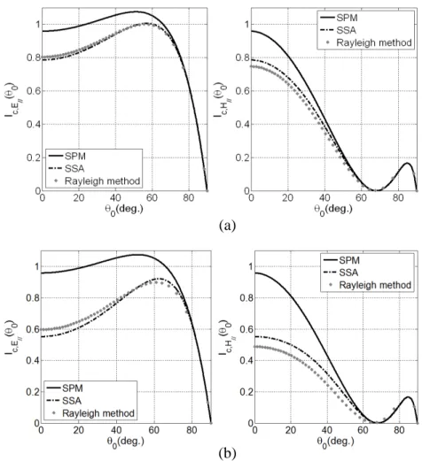
Figure 2(a) shows the coherent intensity for the first configuration under both polarizations and Figure 2(b) gives the curves for the second configuration. For both configurations, the interfaces are uncorrelated with qi,j6=i = 0. The curves show that the coherent intensity is higher in polarization
E//. For both configurations, we notice the Brewster phenomenon in the polarization H// and the coherent intensity becomes smaller under θBrewster = 68.2◦. Under normal incidence, the SPM method
gives the same value under both polarizations. It’s likewise with the SSA model. For the Rayleigh-Fourier method, the coherent intensity under normal incidence depends on the polarization. This result is caused by the anisotropy of one-dimensional surfaces. The differences between the SPM and SSA results increase when increasing the interface roughness and decrease when increasing the incidence angle. Comparison between the SSA model and the Rayleigh-Fourier method is conclusive for the first configuration and satisfactory for the second configuration. The differences are slightly more marked under H//-incidence. For the analysed structure where σ2 = 3σ1/4 and σ3 = 5σ1/8, the SSA model
allows describing the coherent intensity when the rms-height σ1 is smaller about 0.06λ. This value
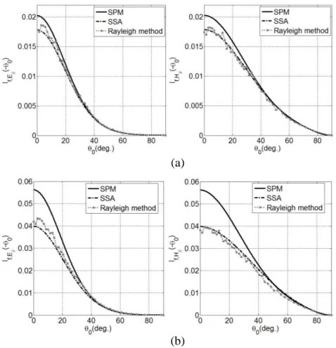
Figure 3(a) shows the backscattered intensity for the first configuration under both polarizations and Figure 3(b) gives results for the second configuration. For both configurations, the interfaces are uncorrelated. The curves show that the backscattered intensity is higher in polarization H//. For both configurations, we do not notice effects of the Brewster phenomenon under the polarization H//. Under normal incidence, the SPM method gives the same value under both polarizations. It is likewise with the SSA model. The differences between the SPM and SSA results increase when increasing the interface roughness. Comparison between the SSA model and the Rayleigh-Fourier method is conclusive for the first configuration and satisfactory for the second configuration. For the second configuration, the SSA method underestimates the numerical method results in polarization E// and overestimates results in polarization H//. For the studied configurations where σ2 = 3σ1/4 and σ3 = 5σ1/8, the SSA model
allows describing the backscattered intensity when the rms-height σ1 is smaller than 0.06λ. This limit value is empirical and obtained by comparison with the Rayleigh-Fourier method results. It can change from one structure to another according to the permittivity and layer thickness values. The SPM model applied with σ1 = 0.06λ does not allow a satisfactory prediction of the backscattered coefficient. The
SPM model gives a satisfactory estimation for heights twice smaller.
Figure 4(a) gives the incoherent intensity obtained with the three methods for the second configuration under the polarization E//. Figure 4(b) shows curves in polarization H//. The incidence
(a)
(b)
Figure 2. Coherent intensity versus incidence angle for (a) the first configuration and (b) the second configuration.
(a)
(b)
Figure 3. Backscattered intensity versus incidence angle for (a) the first configuration and (b) the second configuration.
(a) (b)
Figure 4. Incoherent intensity with the three methods for the second configuration under (a) E// -polarization and (b) H//-polarization.
angle θ0 is fixed at 0◦ and the interfaces are partially correlated with a mixing matrice pij as follows: pij = 1/√3 1/√3 1/√3 0 1/√2 1/√2 0 0 1 (60)
According to (5), the parameters qij are defined by:
qij = 1 2/√6 1/√3 2/√6 1 1/√2 1/√3 1/√2 1 (61)
Comparison between the SSA model and the Rayleigh-Fourier method is satisfactory for both polarizations. The SSA model underestimates the numerical method results in polarization E// and overestimates results in polarization H//. The SPM model does not allow a satisfactory prediction of the incoherent intensity.
8. CONCLUSION
In this paper, we considered the electromagnetic wave scattering from layered structures with an arbitrary number of rough interfaces. First, we applied a perturbation method on the boundary value problem and determined the scattering amplitudes in each medium from recurrence relations. Second, the scattering amplitudes under the first-order small slope approximation are deduced from results derived from the first-order small perturbation method. In final, we determined the closed-form formulae for the coherent and incoherent intensities in the air. The SPM only requires the knowledge of roughness spectra of interfaces and their cross-spectral density. The SSA model requires the knowledge of the correlation and of the two-point height probability distribution. We considered Gaussian height distributions.
We studied configurations with three interfaces. The differences between the coherent intensities obtained from the SPM and SSA models increase when increasing the interface roughness and decrease when increasing the incidence angle. It is likewise observed on the incoherent intensities. We compared the SPM and SSA models with a Rayleigh-Fourier method based on the combination of elementary scattering matrices of different interfaces. For the analyzed structures, we showed that the SSA model can describe the coherent and incoherent intensities for heights twice higher than those obtained by the SPM model.
REFERENCES
1. Elson, J. M., “Infrared light scattering from surfaces covered with multiple dielectric overlayers,”
Appl. Opt., Vol. 16, No. 11, 2873–2881, 1977.
2. Elson, J. M., J. P. Rahn, and J. M. Bennett, “Relationship of the total integrated scattering from multilayer-coated optics to angle of incidence, polarization, correlation length, and roughness cross-correlation properties,” Appl. Opt., Vol. 22, No. 20, 3207–3219, 1983.
3. Amra, C., G. Albrand, and P. Roche, “Theory and application of antiscattering single layers: Antiscattering antireflection coatings,” Appl. Opt., Vol. 25, No. 16, 2695–2702, 1986.
4. Amra, C., J. H. Apfel, and E. Pelletier, “Role of interface correlation in light scattering by a multilayer,” Appl. Opt., Vol. 31, No. 16, 3134–3151, 1992.
5. Afifi, S. and M. Diaf, “Scattering by random rough surfaces: Study of direct and inverse problem,”
Optics Comm., Vol. 265, 11–17, 2006.
6. Tabatabaeenejad, A. and M. Moghaddam, “Bistatic scattering from three-dimensional layered rough surfaces,” IEEE Trans. Geosci. Remote Sens., Vol. 44, No. 8, 2102–2114, 2006.
7. Brelet, Y. and C. Bourlier, “SPM numerical results from an effective surface impedance for a one-dimensional perfectly-conducting rough sea surface,” Progress In Electromagnetics Research, Vol. 81, 413–436, 2008.
8. Imperatore, P., A. Iodice, and D. Riccio, “Electromagnetic wave scattering from layered structures with an arbitrary number of rough interfaces,” IEEE Trans. Geosci. Remote Sens., Vol. 47, No. 4, 1056–1072, 2009.
9. Lin, Z. W., X. J. Zhang, and G. Y. Fang, “Theoretical model of electromagnetic scattering from 3D multi-layer dielectric media with slightly rough surfaces,” Progress In Electromagnetics Research, Vol. 96, 37–62, 2009.
10. Afifi, S., R. Duss´eaux, and R. de Oliveira, “Statistical distribution of the field scattered by rough layered interfaces: Formulae derived from the small perturbation method,” Waves in Random and
Complex Media, Vol. 20, No. 1, 1–22, 2010; Erratum: Waves in Random and Complex Media,
Vol. 20, No. 2, 332, 2010.
11. Afifi, S. and R. Duss´eaux, “On the co-polarized phase difference of rough layered surfaces: Formulae derived from the small perturbation method,” IEEE Trans. Antennas Propagat., Vol. 59, No. 7, 2607–2618, 2011.
12. Afifi, S. and R. Duss´eaux, “On the co-polarized scattered intensity ratio of rough layered surfaces: The probability law derived from the small perturbation method,” IEEE Trans. Antennas
Propagat., Vol. 60, No. 4, 2133–2138, 2012.
13. Voronovich, G., Wave Scattering from Rough Surfaces, Springer, Berlin, 1994.
14. Berginc, G. and C. Bourrely, “The small-slope approximation method applied to a three-dimensional slab with rough boundaries,” Progress In Electromagnetics Research, Vol. 73, 131–211, 2007.
15. Luo, G. and M. Zhang, “Investigation on the scattering from one-dimensional nonlinear fractal sea surface by second-order small-slope approximation,” Progress In Electromagnetics Research, Vol. 133, 425–441, 2013.
16. Tsang, L., J. A. Kong, and K.-H. Ding, Scattering of Electromagnetic Waves — Theory and
Application, Wiley-Interscience, New York, 2001.
17. Beckmann, P. and A. Spizzichino, The Scattering of Electromagnetic Waves from Rough Surfaces, Oxford, Pergamon, 1963.
18. Pinel, N. and C. Bourlier, “Scattering from very rough layers under the geometric optics approximation: Further investigation,” J. Opt. Soc. Am. A., Vol. 25, No. 6, 1293–1306, 2008. 19. Duss´eaux, R., P. Chambelin, and C. Faure, “Analysis of rectangular waveguide H-plane junctions
in a nonorthogonal coordinate system,” Progress In Electromagnetics Research, Vol. 28, 205–229, 2000.
20. Kuo, C.-H. and M. Moghaddam, “Electromagnetic scattering from multilayer rough surfaces with arbitrary dielectric profiles for remote sensing of subsurface soil moisture,” IEEE Trans. Geosci.
Remote Sens., Vol. 45, No. 2, 349–366, 2007.
21. Petit, R., Ed., Electromagnetic Theory of Gratings, Springer-Verlag, Heidelberg, 1980.
22. Van Den Berg, P. M. and J. T. Fokkema, “The Rayleigh hypothesis in the theory of diffraction by a perturbation in a plane surface,” Radio Sci., Vol. 15, 723–732, 1980.
23. Baudier, C. and R. Duss´eaux, “Scattering of an E//-polarized plane wave by one-dimensional rough surfaces: Numerical applicability domain of a Rayleigh method in the far-field zone,” Progress In
Electromagnetics Research, Vol. 34, 1–27, 2001.
24. Mainguy, S. and J. J. Greffet, “A numerical evaluation of Rayleigh theory applied to scattering by randomly rough dielectric surfaces,” Waves in Random Media, Vol. 8, No. 1, 79–101, 1998.
25. Born, M. and E. Wolf, Principles of Optics — Electromagnetic Theory of Propagation Interference
and Diffraction of Light, Pergamon, Oxford, 1980.
26. Tsang, L., J. A. Kong, K. H. Ding, and C. O. Ao, Scattering of Electromagnetic Waves — Numerical