HAL Id: hal-00317030
https://hal.archives-ouvertes.fr/hal-00317030
Submitted on 1 Jan 2003
HAL is a multi-disciplinary open access
archive for the deposit and dissemination of
sci-entific research documents, whether they are
pub-lished or not. The documents may come from
teaching and research institutions in France or
abroad, or from public or private research centers.
L’archive ouverte pluridisciplinaire HAL, est
destinée au dépôt et à la diffusion de documents
scientifiques de niveau recherche, publiés ou non,
émanant des établissements d’enseignement et de
recherche français ou étrangers, des laboratoires
publics ou privés.
regimes of the Iberian Peninsula
L. Morala, A. Serrano, J. A. Garcia
To cite this version:
L. Morala, A. Serrano, J. A. Garcia. Detecting quasi-oscillations in the monthly precipitation regimes
of the Iberian Peninsula. Annales Geophysicae, European Geosciences Union, 2003, 21 (3), pp.819-832.
�hal-00317030�
Annales
Geophysicae
Detecting quasi-oscillations in the monthly precipitation regimes of
the Iberian Peninsula
L. Morala, A. Serrano, and J. A. Garc´ıa
Departamento de F´ısica, Facultad de Ciencias, Universidad de Extremadura, Badajoz, Spain Received: 13 May 2002 – Revised: 26 August 2002 – Accepted: 28 August 2002
Abstract. A spectral analysis of the time series
correspond-ing to the main monthly precipitation regimes of the Iberian Peninsula was performed using two methods, the Multi-Taper Method and Monte Carlo Singular Spectrum Analy-sis. The Multi-Taper Method gave a preliminary view of the presence of signals in some of the time series. Monte Carlo Singular Spectrum Analysis discriminated between potential oscillations and noise.
From the results of the two methods it is concluded that there exist three significant quasi-oscillations at the 95% level of confidence: a 5.0 year quasi-oscillation and a long-term trend in the Atlantic pattern of March, a 3.2 year quasi-oscillation in the Cantabrian pattern of January, and a 4.0 year quasi-oscillation in the Catalonian pattern of Febru-ary. These quasi-oscillations might be related to climatic variations with similar periodicities over the North Atlantic Ocean.
The possible simultaneity of high values of precipitation generated by the significant quasi-oscillations and high sea– level pressures was studied by means of composite maps. It was found that high values of precipitation generated by the oscillations of the Atlantic patterns of January and March ex-ist simultaneously with a specific high pressure structure over the North Atlantic Ocean, that allow cyclonic perturbations to cross the Iberian Peninsula. During the non-wet years, this high pressure structure moves northwards, keeping the track of the low pressure centers to the north, far from the Iberian Peninsula.
On the other hand, high values of precipitation generated by the oscillation of the Cantabrian pattern of January exist simultaneously with a high pressure structure over the Gali-cia region and the Cantabrian Sea, that allow a northerly flow over the region.
Also, a positive trend in the NAO index for March has been found, starting in the sixties, which is not evident for other winter months. This trend agrees with the decreasing trend found in the March Atlantic pattern.
Correspondence to: J. A. Garc´ıa (agustin@unex.es)
Key words. Meteorology and atmospheric dynamics
(cli-matology; precipitation) Oceanography: general (climate and interannual variability)
1 Introduction
Precipitation is a very irregular variable. It presents a wide variability both spatially and temporally at very different scales (interannual and intraannual). This is particularly true for the Iberian Peninsula, whose geographical location (be-tween two sources of humidity: the Atlantic Ocean and the Mediterranean Sea) and the existence of various mountain chains add difficulties to the construction of a precipitation model. However, the great influence of precipitation on life in the Iberian Peninsula (agriculture, water supply, the tourist trade, etc.) makes it of great importance to understand the causes of this variability. In this sense, the detection of oscil-lations in precipitation time series is a very interesting topic, not only for predictive purposes, but also because it yields important information for the understanding of climate, since the oscillations can be seen as responses of the climate sys-tem to external forcing or feedback processes.
Precipitation over the Iberian Peninsula shows a strong seasonal character which affects its nature (frontal or convec-tive). This is due to the fact that some factors become impor-tant only during some months of the year. Thus, while pre-cipitation during winter can be mostly explained by synoptic-scale perturbations crossing the Iberian Peninsula, local fac-tors generating convective storms must be taken into account for the understanding of Spring, Summer and Autumn pre-cipitation. This situation suggests considering separately each calendar month in order to improve the characteriza-tion of the precipitacharacteriza-tion regimes in the Iberian Peninsula. This was done by Serrano et al. (1999a), who showed that some monthly precipitation regimes exist only during certain months of the year, and vanish for others.
In the present paper a spectral analysis of those signifi-cant monthly precipitation regimes is performed. The aim is
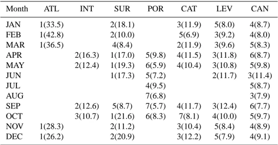
Table 1. Rank and percentage of total variance explained (in parentheses) by PCs that are associated with common patterns. Blank spaces
correspond to months where the pattern was not detected
Month ATL INT SUR POR CAT LEV CAN
JAN 1(33.5) 2(18.1) 3(11.9) 5(8.0) 4(8.7) FEB 1(42.8) 2(10.0) 5(6.9) 3(9.2) 4(8.0) MAR 1(36.5) 4(8.4) 2(11.9) 3(9.6) 5(8.3) APR 2(16.3) 1(17.0) 5(9.8) 4(11.5) 3(11.8) 6(8.7) MAY 2(12.4) 1(19.3) 6(5.9) 4(10.4) 3(10.8) 5(9.8) JUN 1(17.3) 5(7.2) 2(11.7) 3(11.4) JUL 4(9.5) 5(8.7) AUG 7(6.8) 3(7.9) SEP 2(12.6) 5(8.7) 7(5.7) 4(11.7) 3(12.4) 6(7.7) OCT 3(10.7) 1(21.6) 6(8.3) 7(8.1) 4(10.0) 5(9.7) NOV 1(28.3) 2(11.2) 3(10.4) 5(8.4) 4(8.9) DEC 1(26.2) 2(20.9) 3(12.2) 5(7.9) 4(9.1)
the detection of significant quasi-oscillations in the monthly precipitation series over the Iberian Peninsula by analyzing separately each calendar month. This study allows for the identification of time characteristics specific to some months that might be masked in annual or seasonal analyses.
There have been studies aimed at detecting oscillations in the main precipitation regimes in the Iberian Peninsula. However, they deal with annual series (Rodr´ıguez-Puebla et al., 1998) or with continuous quarterly series (Garc´ıa et al., 2002). Since some spatial regimes of precipitation are only reliable for certain calendar months, an analysis for each month, as is performed in the present paper, seems to be more suitable.
The time analysis was carried out using two modern tech-niques of time series spectral analysis: MTM (the Multi-Taper Method) and SSA (Singular Spectrum Analysis). The great number of data series to be analyzed suggested first making a preliminary exploration of the spectra. For this pur-pose, we used the MTM, which generates a first selection of quasi-cycles that later will be studied in detail using an SSA, in particular the Monte Carlo SSA test (Allen and Smith, 1996). Finally, we will describe the results of a search for a relationship between the resulting statistically significant quasi-cycles and some climatic variable, in order to explain the origin of the oscillations.
We will begin by describing briefly the data and the spec-tral analysis methods employed in this work (MTM and SSA).
2 Data
Precipitation is a very complicated variable to deal with. In the case of the Iberian Peninsula, for instance, its descrip-tion involves a large range of temporal and spatial scales. The highly seasonal nature of its precipitation field suggests studying each calendar month separately, since no precipita-tion seasons could be defined a priori for all the staprecipita-tions. In
order to study the evolution of the precipitation field and its possible teleconnections, the main modes of variation of pre-cipitation over the Iberian Peninsula identified and character-ized by Serrano et al. (1999a) were used in this work. These modes of variation are preferred over the individual station records, since they better represent the general main precipi-tation regimes and are less noisy than the local records.
The main modes of variation of precipitation, which are the basis of this study, were obtained by applying Princi-pal Component Analysis (PCA) to forty precipitation station records covering the Iberian Peninsula from 1919 to 1992 (Serrano et al., 1999a). Thirty-five precipitation series were provided by the Instituto Nacional de Meteorologia of Spain, four by the Instituto Nacional de Meteorologia e Geofisica of Portugal and one by the Real Instituto y Observatorio de la Armada Espa˜nola of Spain. The modes of variation were obtained for each calendar month separately. The PCs were rotated using the Varimax method. Direct Oblimin and Pro-max were also tested. Since there were no significant differ-ences between the rotated PCs, the simpler and widely used Varimax method was preferred.
Under the hypothesis that the PCs are linked to general circulation conditions that vary slowly throughout the year, main patterns must remain relevant for various months. Ac-cordingly, only those spatial patterns appearing during at least two contiguous calendar months were retained. Thus, taking into account the different months, 57 modes of vari-ation were selected. These modes of varivari-ation correspond to seven different precipitation patterns: ATL (Atlantic), INT (Interior), SUR (South), POR (Galicia and North-ern Portugal), CAT (Catalonia), LEV (Levante) and CAN (Cantabrian).
The rank in the PCA, the percentage of total variance ex-plained and the pattern they are associated with of the 57 modes of variation are listed in Table 1. Note that not all pat-terns are detected in each calendar month. It can be seen that during summer only POR and CAN patterns are found. This is due to the increasing importance of local factors which
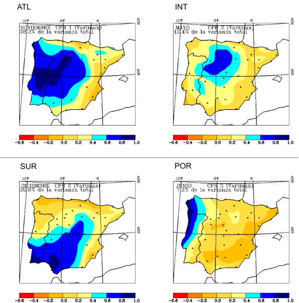
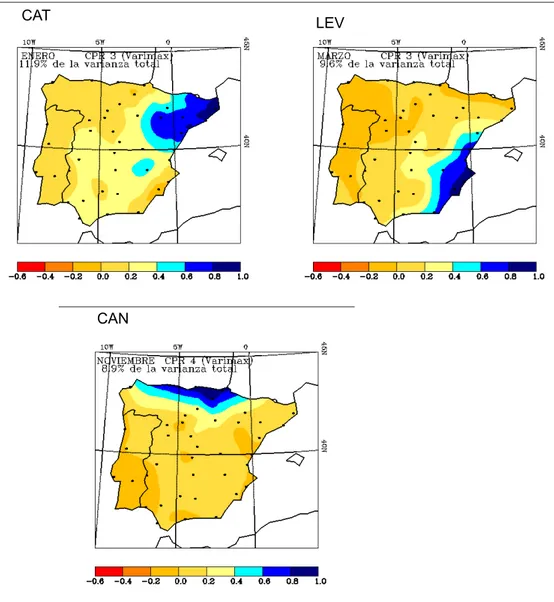
ATL INT
SUR POR
Fig. 1. Examples of loading maps of the ATL, INT, SUR, POR, CAT, LEV, and CAN patterns. The text gives the month where the pattern
appears and the percentage of variance explained by the pattern for that month.
block the detection of wide, spatially coherent patterns of precipitation. In Fig. 1 an example of the spatial distribution loading for each pattern is shown. The loading value repre-sents the correlation between the station series and the PC, since Hotelling normalization was used (Jollife, 1986).
These 57 modes of variation associated with seven differ-ent precipitation patterns constitute a suitable description of the monthly precipitation field over the Iberian Peninsula and are the basis of the present study. For a more detailed de-scription of these modes of variation, please refer to Serrano et al. (1999a).
3 Spectral analysis methods
While a time series can be analyzed in either the time-domain or the frequency-domain, the latter is usually more inter-esting, because the relevant temporal scales of the different
physical processes are easier to distinguish. In order to obtain a good estimate of the distribution of the power (variance) of the series versus frequency (the power spectral density), it is reasonable to apply independent methods. We selected the following:
1. The Multi-Taper Method (MTM);
2. Singular Spectrum Analysis (SSA): the Monte Carlo SSA test (MCSSA).
3.1 Multi-Taper Method (MTM)
The purpose of this non-parametric spectral method (Thom-son, 1982) is to compute a set of independent and signifi-cant estimates of the power spectrum, in order to obtain a better and more reliable estimate for finite time series than with single-taper methods. The MTM provides high spec-tral resolution, as well as statistical confidence levels for the
CAT LEV
CAN
Fig. 1. Continued ....
spectral peaks it detects. It is thus superior to the classical Blackman-Tukey method, which yields a much lower reso-lution, and because the confidence levels are independent of the peak amplitudes. The MTM has been applied to various fields: Earth sciences, (Lindberg, 1986; Park et al., 1987), geophysics (Lanzerotti et al., 1986), climatology on inter-decadal and century time scales (Kuo et al., 1990; Ghil and Vautard, 1991; Mann et al., 1995) and paleoclimatology with tree-ring data (Thomson, 1990b), marine core data (Thom-son, 1990a; Berger et al., 1991), and ice core data (Yiou et al., 1995).
The method, devised by Thomson (1982) based on the work of Slepian (1978), consists of objectively finding tapers in order to minimize the spectral leakage of the power spec-trum outside a pre-determined bandwidth. Thomson also shows that only K = 2p − 1 tapers are resistant to spec-tral leakage, where p is the the half-bandwidth expressed in Rayleigh frequency units. Thus, only K tapers are used in the calculations.
The method provides an unbiased estimate of the ampli-tude in the case of a white-noise background, and is robust to different types of noise and signal patterns. Once the MTM spectrum has been obtained it is necessary to isolate any pe-riodic signal corresponding to singular peaks in the power spectrum. This is accomplished by Thomson’s (1982) re-shaping procedure with some slight modifications (Mann and Lees, 1996): the robust noise background estimation proce-dure. This procedure uses a median-smoothed MTM spec-trum of the time series in order to provide an estimate of the underlying noise background. Assuming that this noise was generated by an AR(1) red noise process, the true noise back-ground is obtained by fitting an analytical red noise spectrum to the median-smoothed background estimate. Finally, the significance of periodic or quasi-periodic peaks in the spec-trum relative to the estimated red noise background is gauged by using elementary sampling theory (Percival and Walden, 1986). Elementary sampling theory, used with a single data taper by Gilman et al. (1963) in their investigation of red
noise confidence testing in climate spectra, assumes that the spectra are χ2 distributed with ν degrees of freedom in the spectral estimate. For the adaptive multi-taper spectrum esti-mate ν ≈ 2K. The ratio of power associated with a peak in the spectrum to the local power level of the background noise is assumed to be distributed as χν2, and can be compared to the tabulated χ2 probability distribution to determine peak significances.
3.2 Singular Spectrum Analysis (SSA): a tool for studying dynamical systems
Singular Spectrum Analysis (SSA) is a data-adaptive method based on the idea of sliding a window down a time series and looking for patterns that account for a high proportion of the variance of the series obtained. This analysis is closely re-lated to the technique of principal component analysis. The original purpose of SSA was noise reduction in the anal-ysis of experimental data and was first applied to nonlin-ear dynamics by Broomhead and King (1986). Paleocli-matic records were analyzed by SSA by Fraedrich (1986) and Fraedrich and Ziehmann-Schlumbohm (1994), who ob-served that the algorithm could be used to estimate the num-ber of degrees of freedom necessary to model the dynamics of an attractor. Vautard and Ghil (1989) refined SSA and applied it to four long marine cores. They emphasized the direct physical interpretation of the individual EOFs (empiri-cal orthogonal functions) obtained with SSA, introducing the idea of searching for pairs of sinusoidal EOFs in quadrature, which were taken to indicate a physical oscillation. Various other records have been analyzed through SSA (the histor-ical global temperature record, the Southern Oscillation in-dex) with the introduction of improvements in distinguish-ing signals from noise. One such problem had been the lack of effective statistical tests to discriminate between potential oscillations and noise. Allen and Smith (1996, henceforth AS96) found that the basic formalism of SSA provides a nat-ural test for modulated oscillations against an arbitrary col-ored noise null hypothesis: the Monte Carlo SSA test (MC-SSA).
3.2.1 Applications of SSA
1. Detecting signals. A natural application of SSA is de-tecting the signal in a time series. By plotting the eigen-values in decreasing order, one can identify those EOFs dominated by a signal and those dominated by noise, discriminating between high variance oscillations and a steep slope, and noise characterized by low variances and a flat floor. The occurrence of a pair of high-ranked eigenvalues indicates the possible presence of a phys-ically meaningful deterministic oscillation. While it is effective at separating signals from pure white noise, the rank-order is unreliable for systems contaminated with red noise or for nonlinear systems, in general. High-ranked pairs could be spurious pairs. We need to decide on the confidence level to reject the null hypothesis that
the features identified are attributable to the stochastic component of the record. There are two ways to test for statistical significance (Elsner and Tsonis, 1996): an-alytically or with the use of a Monte Carlo approach. Analytical methods involve assumptions about the dis-tribution of the particular random variable being used as the test statistic. The distribution statistics on random variables from SSA will, in general, be non-Gaussian and therefore difficult to describe analytically. An ac-ceptable way around this problem is to use the Monte Carlo approach. The Monte Carlo SSA test involves generating surrogate records from a model based on the null hypothesis, see AS96 for details. The application of the MCSSA test can be summarized as follows. The first step in MCSSA is to assume a noise model. Since a large class of geophysical processes generate series with large power at the lower frequencies (AS96), a red noise is a convenient model to begin with. From the time series x(t ), the parameters of the red noise are de-termined by a maximum-likelihood criterion. In order to test the statistical significance of a signal against the null hypothesis selected, an ensemble of surrogate time series is generated with the parameters obtained in the above step. At each Monte Carlo step an autocovari-ance matrix CRis computed. These covariance matrices
are projected onto the EOFs of the actual data yielding an ensemble of eigenvalues from which the confidence intervals are obtained. Usually the 2.5 and 97.5 per-centiles are computed. If an eigenvalue λk lies outside
this confidence interval, the time series can be consid-ered to be different from the generic red noise simula-tion at the 95% level of significance.
As pointed out in AS96, the main problem with the above procedure is that data and surrogates are not treated in the same way, since both the data covariance matrix and the surrogate covariance matrices are pro-jected onto the data EOFs. This compresses the variance into the highest-ranked EOFs in the data but not in the surrogates, since it is implicitly assumed that none of the data is noise. AS96 introduces a variant of the MC-SSA method which is based on the assumption that all the data is noise, except that which has previously been established as signal. The procedure followed is then the same as before, except that data covariance matrix and surrogate covariance matrices are projected onto the null hypothesis basis, which is assumed initially to be red noise. If some of the data eigenvalues lie above the 97.5 percentile of their corresponding surrogate er-ror bar, the data are taken to be inconsistent with the null hypothesis and those eigenvalues with their corre-sponding EOFs are taken as a signal. Once an eigen-value and the corresponding EOF is taken as signal, a new Monte Carlo test is carried out including the EOFs found to be significant in the null-hypothesis, to check for other features in the spectrum which may have been concealed by that signal. This procedure is repeated
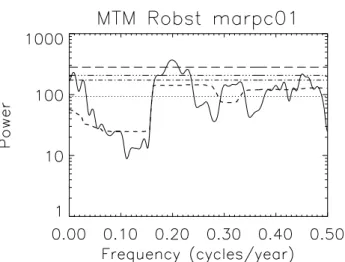
un-Fig. 2. Significant results of MTM for the pattern of March (ATL).
The continuous line is the adaptive MTM spectrum; the various dis-continuous lines are the median-smoothed spectrum (thick-dashed line), and the curves associated with the 50%, 90%, 95%, and 99% confidence levels.
til a null-hypothesis that cannot be rejected is reached. 2. Filtering and reconstructing the time series. Another
application of SSA is to filter the time series, reducing the background noise without losing any significant por-tion of the signal. Because the eigenvectors of the time series are not assumed to be sinusoidal, as in the case of the basis functions used in Fourier analysis meth-ods, filtering with SSA is sometimes described as data-adaptive. Projecting the original time series onto the individual eigenvectors, one has the temporal principal components in each direction, which in SSA terms are called T-PCs. It is possible to reconstruct a filtered ver-sion of the time record based only on the significant T-PCs. We take the set of dominant principal components and construct a filtered time series equal in length to the original series. The background noise is substantially reduced in this filtered time series. Then analysis by the Maximum Entropy Method (MEM), a high resolution spectral method, clearly reveals the frequency of the os-cillations.
In sum, the procedure of the spectral analysis performed in this work will be first, to detect the significant oscillations by using the MCSSA test; second, to filter and to reconstruct the time series including only the detected signals; and finally, to analyze the reconstructed series using the Maximum Entropy Method (MEM).
4 Results
Due to the great number of time series (57), we shall ex-plain in detail the procedure for one of them. The results for the complete set of series will be summarized in the corre-sponding tables. The example that we shall use to explain
the procedure is the series corresponding to the Atlantic pat-tern of March. One of the reasons for using March ATL is that, at the end of the analysis, this case was found to be very interesting. The SSA-MTM toolkit (Dettinger et al., 1995) was used to carry out both the MTM and MCSSA spectral analyses.
4.1 Multi-Taper Method
Due to the shortness of our series (only 74 years), the MTM was performed using p = 2 (i.e. a bandwidth of 4/74 cy-cles/year) and K = 3. The robust red noise assumption was taken and the adaptive MTM spectrum was constructed. The spectrum was smoothed with a window of 0.15 cycles/year. Then a red noise model was fitted to the smoothed spectrum, obtaining the curves associated with the 90%, 95%, and 99% confidence levels. The signals are then defined as the parts of the spectrum lying above the 99% curve.
4.1.1 MTM results
Figure 2 shows the MTM graph for the March ATL pat-tern, consisting of the power spectrum, the smoothed spec-trum, and the confidence levels. The significant quasi-cycles are those whose power surpasses the 99% confidence level. The intervals of the significant quasi-cycles at the 99% con-fidence level are summarized in Table 2. Time series with no significant signals are represented by [—]. One notes that the ATL pattern presents significant periods in 4 of the 5 months in which it appears. Similarly, the SUR pattern appears in 10 months and has significant periods in 7 of them. By con-trast, the CAN pattern is present during the whole year but has significant periods in only 2 months.
Most of the periods are between 2 and 6 years. Only two lie outside this interval (8 and 12 years). There are six months with one significant period: February (4 years), March (5 years), April (2.5 years), June (3.5 years), Septem-ber (3.5 years), and OctoSeptem-ber (3.5 years). There are two months without any significant period: July and August, the summer months. And there are four months with two signif-icant periods: January (3 and 8 years), May (5 and 12 years), November (2 and 6 years), and December (2.5 and 6 years). The most frequent period is 3.5 years (7 events), followed by 2.5 years (6 events).
The MTM has thus reduced the initial set of 57 time series to a set of 27 series with significant oscillations. The follow-ing step is to study these 27 series in detail usfollow-ing MCSSA. 4.2 MCSSA test: finding significant signals
4.2.1 March (ATL)
1. One has first to apply data-adaptive MCSSA to find the data EOFs associated with the significant pure noise EOFs. Then, projecting both the data and 10 000 sur-rogate series onto the data eigenbasis ED with a
win-dow width of M = 15, and using 2.5 and 97.5 per-centile limits, one obtains the data-adaptive
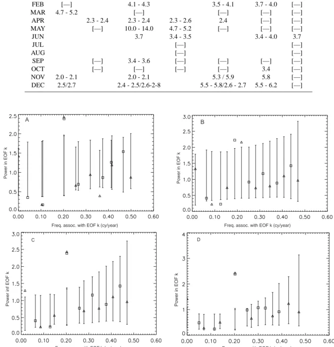
eigenval-Table 2. MTM significant quasi-periods (year/cycle). Time series with no significant signal are represented by [—]
Month ATL INT SUR POR CAT LEV CAN
JAN 3.5 - 3.8 [—] 8.3 [—] 3.1 - 3.2 FEB [—] 4.1 - 4.3 3.5 - 4.1 3.7 - 4.0 [—] MAR 4.7 - 5.2 [—] [—] [—] [—] APR 2.3 - 2.4 2.3 - 2.4 2.3 - 2.6 2.4 [—] [—] MAY [—] 10.0 - 14.0 4.7 - 5.2 [—] [—] [—] JUN 3.7 3.4 - 3.5 3.4 - 4.0 3.7 JUL [—] [—] AUG [—] [—] SEP [—] 3.4 - 3.6 [—] [—] [—] [—] OCT [—] [—] [—] [—] 3.4 [—] NOV 2.0 - 2.1 2.0 - 2.1 5.3 / 5.9 5.8 [—] DEC 2.5/2.7 2.4 - 2.5/2.6-2-8 5.5 - 5.8/2.6 - 2.7 5.5 - 6.2 [—] A
Freq. assoc. with EOF k (cy/year)
Power in EOF k
Freq. assoc. with EOF k (cy/year)
Power in EOF k
B
Freq. assoc. with EOF k (cy/year)
Power inf EOF k
C
Freq. assoc. with EOF k (cy/year)
Power in EOF k
D
Fig. 3. Monte Carlo SSA of March (ATL): projection onto (a) the data-adaptive basis, (b) red noise null hypothesis basis, (c) composite
null hypothesis basis (including data EOFs 1 and 2), (d) composite null hypothesis basis (including data EOFs 1, 2 and 3). In all cases the window length was M = 15 yr. The error bars denote 97.5 and 2.5 percentiles of a 10 000 surrogate series.
ues and the surrogate data bars. These are plotted against the frequency associated with their correspond-ing EOFs. Since SSA EOFs are not pure sinusoidal functions, identifying a single frequency with each EOF is not straightforward. The association is made by max-imizing the squared correlation with a sinusoidal
func-tion. If the correlation is maximum with a sine function, the EOF is odd and the corresponding eigenvalue will be plotted with a square. If the correlation is maximum with a cosine function, the EOF is even and the eigen-value is plotted with a triangle. A sine-cosine oscillatory pair thus appears when two eigenvalues (a square and a
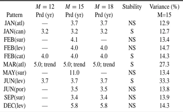
Table 3. Summary of MCSSA test results, with M = 15
Pattern Periods (years)
JAN(atl) 3.7 JAN(can) 3.2 FEB(sur) 4.1 FEB(lev) 4.0 FEB(cat) 4.0 MAR(atl) 5.0; trend MAY(sur) 11.0 JUN(lev) 3.7 JUN(por) 3.5 SEP(sur) 3.4 DEC(lev) 5.8
triangle) lie above their surrogate data bars. In Fig. 3a one sees that the first and second EOFs are significant and are located just over the 0.20 cycles/year frequency. 2. The MCSSA test of the pure noise null hypothesis (projecting both data and surrogates onto the EN noise
basis) is performed with a window width of M = 15 and 10 000 Monte Carlo surrogate data series. The eigen-values and the surrogate data bars (percentile limits: 2.5, 97.5) are again plotted against the frequency associ-ated with their corresponding EOFs (Fig. 3b). Note how the EOFs of the red noise covariance matrix are regu-larly separated by almost exactly 1/(2M). A sine-cosine oscillatory pair appears around the 0.20 cycles/year fre-quency. They are close together but not superimposed. This appearance of at least one significant eigenvalue is indicative of the presence of a quasi-oscillation different from noise.
Comparing the data-adaptive projection (Fig. 3a) with the pure noise projection (Fig. 3b) shows that the data EOFs 1 and 2 are associated with the pure noise EOFs 1 and 2.
3. We then assume that the data EOFs 1 and 2 are associ-ated with the signal, and include them as signal in the
composite null hypothesis. Projection onto the
com-posite null hypothesis basis tends to pair up the sig-nal EOFs just over the frequency corresponding to the quasi-oscillation, in this case 0.20 cycles/year (Fig. 3c). If oscillations other than those included in the null hy-pothesis existed, then new significant oscillatory pairs would appear. These pairs would have to be included in a new null hypothesis in the following iteration of the procedure, continuing the analysis until no new eigen-value appears as significant. In the present case, there is one more significant eigenvalue. It corresponds to the 4th ranked of the data eigenbasis. Its secular pe-riod indicates a trend. We include this new significant EOF into another composite null hypothesis including the 1st, 2nd and 4th data EOFs as signals (Fig. 3d). Now, no further significant eigenvalues have appeared,
Table 4. Analysis using different window widths. M = Window
width (years), Variance: percentage of the reconstructed component with respect to the original series
M =12 M =15 M =18 Stability Variance (%)
Pattern Prd (yr) Prd (yr) Prd (yr) M=15
JAN(atl) — 3.7 3.7 NS 12.9
JAN(can) 3.2 3.2 3.2 S 12.7
FEB(sur) — 4.1 — NS 13.4
FEB(lev) — 4.0 4.0 NS 14.7
FEB(cat) 4.0 4.0 4.0 S 14.3
MAR(atl) 5.0; trend 5.0; trend 5.0; trend S 27.3
MAY(sur) — 11.0 — NS 13.4
JUN(lev) 3.7 3.7 3.7 S 33.3
JUN(por) — 3.5 3.5 NS 13.8
SEP(sur) — 3.4 3.4 NS 13.9
DEC(lev) — 5.8 5.8 NS 14.3
which means that the signal is a quasi-cycle of 5.0 years and a secular trend.
4.2.2 Summary of the results
The results of the applying the preceding process (with M = 15) to each time series are summarized in Table 3. Only these eleven patterns presented significant signals.
It is now necessary to check whether these significant quasi-oscillations are stable against changes in the window width. Some sensitivity of results to window width is in-evitable due to the constraint that the EOFs must be orthog-onal, but if a pair only appears for certain values of M, this is a reason to doubt its significance. But unfortunately, the converse is not true: the stability of an oscillatory pair does not assure its physical significance (Allen and Smith, 1996). The entire process (pure noise projection and composite null hypothesis test) was repeated with M = 12 and M = 18, and some interesting results were found (Table 4) which will be discussed in the following subsection.
4.2.3 The selected quasi-cycles: moving window analysis The analysis of signal stability by changing the window width revealed that not all the pre-selected signals are sta-ble. Table 4 lists the results for the three windows, and shows how there are signals that are significant only for certain win-dows, whereas there are other signals that are significant for all three windows. The table gives the most important char-acteristics of the signals: their stability, the quasi-period, and the variance explained (in the case of M = 15). This vari-ance was computed as the sum of the varivari-ances explained by each of the significant EOFs associated with the quasi-cycle. The signals can thus be classified into “stable” (S), in-dicating the presence of eigenvalues in the three windows, and “non-stable” (N S), indicating the absence of signifi-cant eigenvalues in some window. From Table 4, one
ob-serves four stable quasi-oscillations (January (CAN), Febru-ary (CAT), March (ATL), and June (LEV)). Also, the oscil-lations corresponding to March (ATL) and June (LEV) are well defined (in the sense that they lie clearly above the sur-rogate bars) at M = 15 and M = 18. The rest of the quasi-oscillations seem to be unstable and poorly defined. For that reason, the initial selection of significant quasi-cycles has to be questioned. Observing Table 4, one might conclude that the “best” quasi-cycle is the 3.7 years of June (LEV), be-cause it is stable, well defined (at M = 15 and M = 18), and explains 33.3% of the variance, better than, for example, March (ATL) which, while it is stable, and well defined (at M =15 and M = 18), only explains 27.3% of the variance. That conclusion could be misleading.
Therefore, a moving window analysis is performed in or-der to assess the dates for which the oscillations remain sig-nificant. The moving window analysis slides a window of length S down a series of length N , generating a set of N − S +1 sub-series that will be studied, one by one, with MCSSA. If the oscillation of the original series remains sig-nificant in each of the sub-series, one can conclude that the oscillation is stable over the entire original period (N ), i.e. the oscillation is not a particular event during a certain tem-poral interval that appears as significant in the analysis of the whole period. To this goal, MCSSA was performed with
M = 12 instead of M = 15, since with a moving window
width of S = 61, a lower value of M will preserve the sig-nificance level. The window width S = 61 generates 14 sub-series from each sub-series. These were analysed using MCSSA under the null hypothesis of pure noise.
The results showed that the oscillation of June (LEV) was significant only around the first part of the 1919–1992 period and was not significant in the 1927–1992 period. It seems that the oscillation was so strong in this first part of the time series that it remained significant in the analysis of the whole period. Only by analyzing the sub-series can one delimit the period of existence of the oscillations. In our case, the oscil-lations of January (CAN), February (CAT), and March (ATL) were significant during the whole 1919–1992 period. In all three cases, the significance of the oscillations tended to de-crease in the last years of the period.
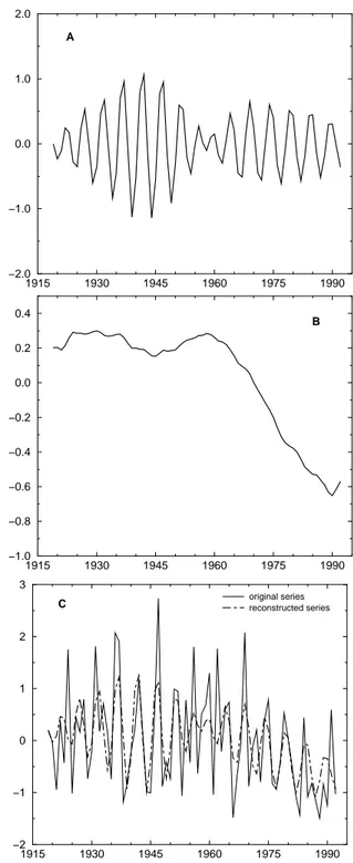
For the case of March (ATL), there was an interesting evo-lution of the ranking of the eigenvalues in the different sub-series. The two eigenvalues (ranked 1 and 2) associated with the quasi-cycle of 5 years remain in this position in all the sub-series. The third position, however, is occupied by an eigenvalue corresponding to a quasi-cycle of 2.5 years and not by the eigenvalue corresponding to the trend, which is situated in the last place of the ranking from sub-series 1 to sub-series 8. In sub-series 9, the eigenvalue corresponding to the secular trend begins to climb in rank, arriving at the third position by sub-series 14. This concurs with the form of the trend (Fig. 4) obtained by reconstructing the series including eigenvalue 3 of the pure noise MCSSA with M = 15 (whole period). One observes that the downward trend starts around the 1960s and continues until the 1990s (the last three years of the series), when it seems to bottom out.
1915 1930 1945 1960 1975 1990 −2.0 −1.0 0.0 1.0 2.0 A 1915 1930 1945 1960 1975 1990 −1.0 −0.8 −0.6 −0.4 −0.2 0.0 0.2 0.4 B 1915 1930 1945 1960 1975 1990 −2 −1 0 1 2 3 original series reconstructed series C
Fig. 4. Reconstructed series for March (ATL): (a) including only
EOFs 1 and 2, corresponding to the quasi-oscillation, (b) including only EOF 3, corresponding to a long-term trend, (c) original time series plus reconstructed signal including EOFs 1, 2, and 3.
The case of January (ATL) is particular and calls for at-tention. When the pure noise MCSSA was performed with M = 12, no significant oscillations were found at the 95% level of confidence. But in the moving window analysis of this series with M = 12 and 95%, there appears a significant eigenvalue in 9 of the sub-series. This result suggested the
0.00 0.10 0.20 0.30 0.40 0.50 Frequency (cy/year) 10−6 10−4 10−2 100 102 Power
MEM January (ATL)
A 0.00 0.10 0.20 0.30 0.40 0.50 Frequency (cy/year) 10−6 10−4 10−2 100 102 Power
MEM January (CAN)
B 0.00 0.10 0.20 0.30 0.40 0.50 Frequency (cy/year) 10−4 10−3 10−2 10−1 100 101 Power
MEM February (CAT)
C 0.00 0.10 0.20 0.30 0.40 0.50 Frequency (cy/year) 10−6 10−4 10−2 100 102 Power
MEM March (ATL)
D
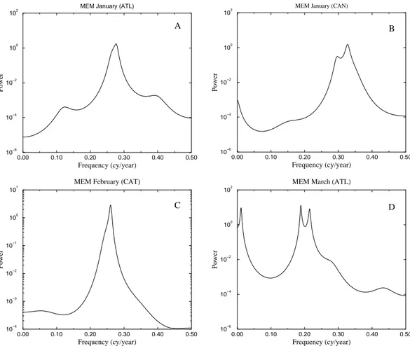
Fig. 5. Maximum Entropy Method (MEM) spectrum of the reconstructed series: (a) MEM spectrum of the reconstructed series of January
(ATL) including only EOF 1, corresponding to a 3.7 year oscillation. (b) MEM spectrum of the reconstructed series of January (CAN) including only EOF 1, corresponding to a 3.4–3.1 year quasi-oscillation. (c) MEM spectrum of the reconstructed series of February (CAT) including EOF 1, corresponding to a 4.0 year oscillation. (d) MEM spectrum of the reconstructed series of March (ATL) including EOFs 1, 2, and 3, corresponding to a long-term trend, and a 5.2–4.7 year quasi-oscillation.
repetition of the analysis at a 90% confidence level. Now, a significant eigenvalue was found for the three windows and in the composite null hypothesis analysis. The oscillation was also significant in the whole set of sub-series of the mov-ing window analysis. For these reasons, this quasi-cycle of 3.7 years of January (ATL) merits inclusion among the se-lected quasi-oscillations.
4.3 Studying the significant signals
Once significant stable signals were found, we could make a detailed study of their associated frequencies. We obtained the filtered time series by reconstruction with the signifi-cant data EOFs. Figure 4 shows the reconstructed quasi-oscillations and the original time series plus the filtered sig-nals for the March (ATL) pattern. These filtered sigsig-nals were analyzed using the Maximum Entropy Method (MEM). Fig-ure 5 shows the different signals. In Fig. 5a, one can observe a clear oscillation of 3.7 years in January (ATL). Figure 5b shows the quasi-oscillation of 3.4–3.1 years (maximum at 3.1 years) present in January (CAN). Figure 5c is the oscillation of 4.0 years of February (CAT). Figure 5d, corresponding
to March (ATL), shows the presence of a trend and a quasi-oscillation of 5.2–4.7 years.
5 Composite maps
Once the oscillations have been identified (quasi-cycles and trends), a composite analysis is performed, in order to detect any sea level pressure structure that occurs simultaneously at high values of the quasi-oscillations found for a certain precipitation regime. This could be a sign of the existence of possible relationships between these oscillations and sea-level pressure (SLP). We applied a composite analysis to the SLP anomalies and tested the average values for a significant difference from the mean using Student’s t-test.
The series with the four best quasi-oscillations were se-lected as index series. The series were reconstructed by in-cluding the EOFs associated with the pure noise significant eigenvalues (i.e. including only the detected quasi-cycles and trends). The composite analysis was performed with:
1. The reconstructed series of January (ATL), including EOF 1 corresponding to the quasi-cycle of 3.7 years;
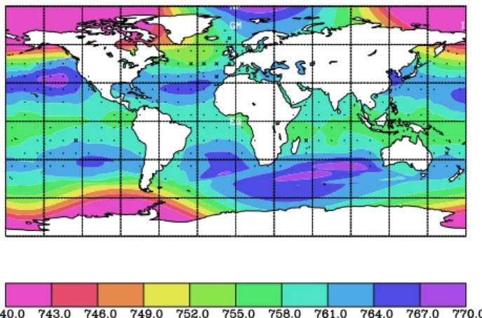
Fig. 6. Composite map of SLP (in mm Hg) for March
correspond-ing to wet years accordcorrespond-ing to the pattern March (ATL). Dots
cor-respond to 10◦×10◦ boxes where Student’s t-test for the
differ-ence in the means of wet and non-wet years was not significant at a confidence level of 99%. Crosses correspond to boxes where that difference was significant.
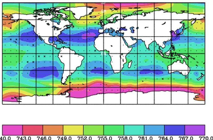
Fig. 7. Composite map of SLP for March corresponding to non-wet
years according to the pattern March (ATL).
2. The reconstructed series of January (CAN), including EOF 1 corresponding to the quasi-cycle of 3.2 years; 3. The reconstructed series of February (CAT), including
EOF 1 corresponding to the quasi-cycle of 4.0 years; 4. The reconstructed series of March (ATL), including
EOFs 1, 2, and 4 corresponding to the quasi-cycle of 5.0 years and the secular trend.
These index series were composited with the sea-level pressure series, obtained from COADS (Comprenhensive Ocean-Atmosphere Data Set, (Woodruff et al., 1987)), for the period 1919–1992 and using boxes of 10◦ latitude × 10◦longitude. A threshold of 0.6 σ separated the wet years from the non-wet years. Using Student’s t-test, with a con-fidence level of 95%, we found that only two reconstructed series showed significant differences between the means of SLP corresponding to wet years and non-wet years: January (ATL) and March (ATL). The composite maps of these series
Fig. 8. Composite map of SLP for January corresponding to wet
years according to the pattern January (ATL).
Fig. 9. Composite map of SLP for January corresponding to
non-wet years according to the pattern January (ATL).
are shown in Figs. 6–9, in which the dots indicate the boxes with no significant values under the t-test and the crosses in-dicate the significant boxes. Less significant but still very interesting are the structures observed in the composite maps corresponding to the reconstructed series of January (CAN). No other significant results were found in the rest of the com-posite maps.
Figures 6 and 7 show the composite maps corresponding to the wet and non-wet years of the reconstructed series of March (ATL). There are four significant boxes, in the area of the North Atlantic Ocean and in the Cantabrian zone. Fig-ures 8 and 9 represent the maps for the wet and non-wet years of the reconstructed series of January (ATL). There are four significant boxes in the Atlantic zone near the Peninsula. The location of the high pressure structures is different during the wet years and during the non-wet years of the same series. There is also a similarity between the structures of the wet years of January (ATL) and of March (ATL), and also of the non-wet years of the same two series.
The two different circulation patterns for wet and non-wet years for the ATL pattern (Figs. 6 and 7 for the case of March, and Figs. 8 and 9 for the case of January) seem to be a
mani-Fig. 10. Composite map of SLP for January corresponding to wet
years according to the pattern January (CAN).
Fig. 11. Composite map of SLP for January corresponding to
non-wet years according to the pattern January (CAN).
festation of the North Atlantic Oscillation (NAO).
The composite maps for the wet years for the ATL pattern (Figs. 6 and 8) show a zonal mean circulation over all the At-lantic Coast of Europe including the Iberian Peninsula, with only the low latitudes being affected by the semipermanent high pressure systems. This situation corresponds to a low NAO index. This atmospheric situation allows cyclonic per-turbations to cross the Peninsula, leading to large amounts of rainfall over Portugal and most of Spain.
These results for January and March agree with the work of Zorita et al. (1992), who found the NAO to be one of the major factors of the winter precipitation over the Iberian Peninsula.
On the contrary, the composite maps for the non-wet years for the ATL pattern (Figs. 7 and 9) show that the high pres-sure belt has expanded northwards to cover the Iberian Penin-sula. This situation corresponds to a high NAO index result-ing from the very high values of the pressure over the Azores. Now, the zonal circulation has moved to higher latitudes with the flows over the Iberian Peninsula being weaker and with a highly meridional character. This keeps the tracks of low pressure systems to the north, far from the Iberian Peninsula,
0.00 0.10 0.20 0.30 0.40 0.50 Freq. assoc. in EOF k (cy/year) 1
10 100
Power in EOF k
SSA NAO MAR
1915 1930 1945 1960 1975 1990 Year −1 0 1 2 NAO MAR RC # 1
Fig. 12. Singular Spectrum Analysis for NAO March (left) and
re-constructed component with EOF 1 (right).
resulting in very dry periods.
The contrary situation occurs for the CAN precipitation regime in January. The wet years (Fig. 10) occur for a high NAO index with a high pressure structure located over the Azores. Under these conditions, the Atlantic air masses cross the Iberian Peninsula from northwest to southeast, leading to precipitation at the northern part of the Cantabric mountain chain, which is the region associated with the CAN pattern. The non-wet years (Fig. 11) correspond to conditions of a low NAO index. In this situation, the Atlantic air masses cross the Iberian Peninsula from southwest to northeast, ar-riving dry and warm at the Cantabrian coast after suffering the Foehn effect over the Cantabrian mountain chain.
It is surprising the decrease in rainfall found for the low frequency component in the ATL pattern in March (Fig. 4). No similar situation is found in any other pattern or month. This decrease in March precipitation over the Iberian Penin-sula has been reported in other works for Portugal (Corte-Real et al., 1998; Trigo and DaCamara, 2000) and for the Iberian Peninsula (Serrano et al., 1999b). In addition, an im-portant increase in the monthly precipitation for the months of March (and October to a lesser extent) on the west coast of Ireland has been reported by Kiely et al. (1998).
In order to look for the causes of this trend, taking into account the suggested relationship between the NAO and the monthly precipitation characterized by the ATL regime, an SSA for the NAO index (based on the difference of normal-ized sea level pressure (SLP) between Ponta Delgada, Azores and Stykkisholmur/Reykjavik, Iceland, see http://www.cgd. ucar.edu/∼jhurrell/nao.html#oseas) for March has been
per-formed. Figure 12 shows the spectrum of eigenvalues versus frequency. It can be seen that the leading eigenvalue is asso-ciated with a trend. The series reconstructed with this eigen-value is shown in Fig. 12. One observes a significant increase in the NAO index from the beginning of the sixties. This be-havior agrees with the decrease shown by the precipitation described by the ATL pattern during March (Fig. 4).
Further SSA analyses were performed on the NAO index for the other winter months (December, January and Febru-ary) and no similar trend was found for any of them, thus, confirming that the trend occurs only in March.
6 Discussion of the results
The use of two quite different methods of spectral analysis allows one to glean more information from the time series. The periods or quasi-periods selected as significant in this work were those that satisfy the requirements for a signal in both methods.
The MTM offered a preliminary view of the characteris-tics of the series, and focused our attention on a group of 27 series and 31 quasi-oscillations. The MTM results were given in Table 2. These quasi-periods are temporal intervals defined by the sections of the spectral peaks that surpass the 99% confidence level. There was a notable absence of pat-terns and quasi-periods during the summer months (July and August) consistent with the very occasional nature of precip-itation in this season. Most of the quasi-periods ranged from 2 to 6 years. Only two of them lay outside this interval: the signal of the CAT pattern of January (8 years) and that of the SUR pattern of May (10–14 years). It has to be kept in mind that since the series are 74 years long, periods longer than 8–10 years have less statistical significance than those of 3–5 years.
The MCSSA results (Table 3) selected only 11 quasi-oscillations, with more precise frequencies, that were within the temporal intervals defined by the MTM. The analysis of the stability of the signals (Table 4) indicated that there are only four stable quasi-cycles (significant eigenvalues for the three windows, 12, 15 and 18 years) at the 95% confidence level:
1. The quasi-oscillation of 3.2 years in the Cantabrian pat-tern of January;
2. The quasi-oscillation of 4.0 years in the Catalonian pat-tern of February;
3. The quasi-oscillation of 5.0 years and a trend in the At-lantic pattern of March;
4. The quasi-oscillation of 3.7 years in the Levante pattern of June;
and one stable quasi-cycle at the 90% confidence level: the quasi-oscillation of 3.7 years in the Atlantic pattern of Jan-uary.
The moving window analysis of the five stable quasi-oscillations showed the quasi-oscillations of January (CAN), Jan-uary (ATL), FebrJan-uary (CAT), and March (ATL) to be de-fined over the whole study period 1919–1992. The quasi-oscillation of June (LEV) appeared to be associated with only the first part of the period (1919–1927): in the rest of the period, the oscillation was not significant. Therefore, we re-jected the oscillation of June.
The reconstruction of the filtered signals (Fig. 4) showed the March (ATL) trend to be clearly downward which could be justified by the increase in the NAO index for that month. The MEM analysis of the reconstructed signals (Fig. 5) showed that the 5.0 year oscillation of March (ATL) ap-peared inside a quasi-oscillation of 5.2–4.7 years. The 3.2
year oscillation of January (CAN) appeared inside a quasi-oscillation of 3.4–3.1 years.
The study of the composite maps of the selected quasi-oscillations indicated that:
1. The high values of precipitation generated by the quasi-cycle of the ATL pattern in March exist simultaneously with a high pressure structure over the North Atlantic Ocean;
2. The high values of precipitation generated by the quasi-cycle of the ATL pattern in January exist simultaneously with that same pressure structure over the North At-lantic Ocean;
3. The high values of precipitation generated by the quasi-cycles of the CAN pattern in January exist simultane-ously with another pressure structure over the Galicia zone and Cantabrian Sea.
Among the significant quasi-oscillations found in this work, the downward trend in March has been reported be-fore for Portugal (Corte-Real et al., 1998; Trigo and DaCa-mara, 2000) and for the Iberian Peninsula (Serrano et al., 1999b). With reference to the rest of the significant oscil-lations, which correspond to short periods between 3 and 5 years, similar results have been reported by Rodriguez-Puebla et al. (1998) using annual time series, and by Garc´ıa et al. (2002) using continuous quarterly data.
As was established before in the composite analysis, sea level pressure patterns which occur simultaneously with the oscillations seem to be related to the NAO. A spectral anal-ysis of the NAO index (Hurrel and Van Loon, 1997; Wun-sch, 1998; Robertson, 2001) reveals a quasi-oscillation with a period of about 2.5 years which is somewhat shorter than ours. However, Tourre et al. (1999), studying spatiotemporal patterns of joint sea surface temperature and sea level pres-sure variability in the Atlantic Ocean, found a 3.5 year pe-riod which corresponds to an SLP dipole-like pattern similar to the NAO, and a 4.4 year period related to pressure anoma-lies located between Iceland and Greenland. Both patterns could affect the strength of westerly winds, and therefore the precipitation regimes, over a large area including the Iberian Peninsula. Also, Venegas and Mysak (2000) found periods around 5 years, 2.7 years and 2.1 years for North Atlantic SLP anomalies.
It is cautiously concluded that the short periods detected in the analysis could be related to the oscillations found in the sea level pressure over the North Atlantic Ocean.
Acknowledgements. This work was supported by the Spanish
CI-CYT under Project CLI99-0845-C03-03. Also thanks are due to the SSA-MTM group for providing us with the SSA-MTM toolkit and to the Spanish Instituto Nacional de Meteorolog´ıa for providing us with the rainfall series.
Topical Editor J.-P. Duvel thanks two referees for their help in evaluating this paper.
References
Allen, M. R. and Smith, L. A.: Monte Carlos SSA: Detecting irreg-ular oscillations in the presence of colored noise, J. Climate, 6, 3373–3402, 1996.
Berger, A. L., M´elice, J. L., and Hinnov, L.: A strategy for fre-quency spectra of Quaternary climate records, Climate Dynam-ics, 5, 227–240, 1991.
Broomhead, D. S. and King, G.: On the Qualitative Analysis of Experimental Dynamical Systems, Adam Hilger, Bristol, 1986. Corte-Real, J., Qian, B., and Xu, H.: Regional climate change in
portugal: Precipitation varibility associated with large-scale at-mospheric circulation, Int. J. Climatol., 18, 619–635, 1998. Dettinger, M., Ghil, M., Strong, C. M., Weibel, C. M., and Yiou,
P.: Software spedites singular-spectrum analysis of noisy time series, Eos, Trans. American Geophysical Union, 76, 12, 14–21, 1995.
Elsner, J. and Tsonis, A.: Singular Spectrum Analysis: A New Tool in Time Series Analysis, Plenum Press, 1996.
Fraedrich, K.: Estimating the dimensions of weather and climate attractors, Atmospheric Science, 43, 419–432, 1986.
Fraedrich, K. and Ziehmann-Schlumbohm, C.: Predictability exper-iments with persistence forecast in red-noise atmosphere, Quart. J. Roy. Meteor. Soc., 120, 387–428, 1994.
Garc´ıa, J. A., Serrano, A., and Gallego, M. C.: A spectral analysis of iberian peninsula monthly rainfall, Theor. Appl. Climatol., 71, 77–95, 2002.
Ghil, M. and Vautard, R.: Interdecadal oscillations and the warm trend in global temperature time series, Nature, 350, 324–327, 1991.
Gilman, D. L., Fuglister, F. L., and Mitchell, J. M. J.: On the power spectrum of red noise, J. Atmos. Sci., 20, 182–184, 1963. Hurrel, J. and Van Loon, H.: Decadal variations in climate
asso-ciated with the north atalntic oscillation, Climatic Change, 36, 301–326, 1997.
Jollife, I.: Principal Component Analysis, Springer-Verlag, 1986. Kiely, G., Albertson, J. D., and Paralange, M. B.: Recent trends in
diurnal variation of precipitation at valentia on the west coast of ireland, J. Hidrol., 208, 1998.
Kuo, C., Lindberg, C. R., and Thomson, D. J.: Coherence estab-lished between atmospheric carbon dioxide and global tempera-ture, Natempera-ture, 343, 709–714, 1990.
Lanzerotti, L., Thomson, D. J., Maclennan, C. G., and Medford, L. V.: Electromagnetic study of the Atlantic continental mar-gin using a section of a trasatlantic cable, J. Geophys. Res., 91, 7417–7427, 1986.
Lindberg, C. R.: Multi-Taper Spectral Analysis of Terrestrial Free Oscillations, Ph.D. thesis, Scripps Institution of Oceanography, University of California, San Diego, 1986.
Mann, M. E. and Lees, J. L.: Robust estimation of background noise and signal detection in climatic time series, Clim. Change, 33, 409–445, 1996.
Mann, M. E., Park, J., and Bradley, R. S.: Global interdecadal and century-scale climate oscillations during the past five centuries,
Nature, 378, 266–270, 1995.
Park, J., Lindberg, C. R., and Vernon III, F. L.; Multi-Taper spectral analysis of high-frequency seismograms, J. Geophys. Res., 92, 12 675–12 684, 1987.
Percival, D. B. and Walden, A. T.; Spectral Analysis for Physi-cal Applications, Cambridge University Press, Cambridge, UK., 1986.
Robertson, A.; Influence of the ocean–atmosphere interaction on the artic oscillation in two general circulation models, J. of Cli-mate, 14, 3240–3254, 2001.
Rodriguez-Puebla, C., Encinas, A. H., Nieto, S., and Garmendia, J.: Spatial and temporal patterns of annual precipitation variability over the iberian peninsula, Int. J. Climatol., 18, 299–316, 1998. Serrano, A., Garc´ıa, J. A., Mateos, V. L., Cancillo, M. L., and
Gar-rido, J.: Monthly Modes of Variation of Precipitation over the Iberian Peninsula, J. Climate, 12, 2894–2919, 1999a.
Serrano, A., Mateos, V. L., and Garc´ıa, J. A.: Trend Analysis of Monthly Precipitation over the Iberian Peninsula for the period 1921–1995, Phys. Chem. Earth (B), 24, 85–90, 1999b.
Slepian, D.: Prolate spheroidal wave functions, Fourier analysis and uncertainty, V. The discrete case, Bell Syst. Tech. J., 57, 1371– 1429, 1978.
Thomson, D.: Quadratic-inverse spectrum estimates: applications to paleoclimatology, Phil. Trans. R. Soc. London A, 332, 539– 597, 1990a.
Thomson, D.: Time series analysis of Holocene climate data, Phil. Trans. R. Soc. London A, 330, 601–616, 1990b.
Thomson, D. J.: Spectrum estimation and harmonic analysis, Proc. IEEE, 70, 1055–1096, 1982.
Tourre, Y. M., Rajagopalan, B., and Kushnir, Y.: Dominant pat-terns of climate variability in the atlantic ocean during the las 136 years, J. of Climate, 12, 2285–2299, 1999.
Trigo, R. M. and DaCamara, C. C.: Circulation weather types and their influence on the precipitation regime in portugal, Int. J. Cli-matol., 20, 1559–1581, 2000.
Vautard, R. and Ghil, M.: Singular Spectrum Analysis in nonlinear dynamics, with applications to paleoclimatic time series, Physica D, 35, 395–424, 1989.
Venegas, S. A. and Mysak, L. A.: Is there a dominant timescale of natural climate variability in the arctic, J. Climate, 13, 3412– 3434, 2000.
Woodruff, S. D., Slutz, R. J., Jenne, R. L., and Steurer, P. M.: A comprehensive ocean-atmosphere data set., Bull. Amer. Meteor. Soc., 68, 1239–1250, 1987.
Wunsch, C.: The interpretation of the short records, with comments on the north atlantic and southern oscillations, Bulletion of the AMS, 80, 245–255, 1998.
Yiou, P., Jouzel, J., Johnsen, S., and Rognvaldsson, O. E.: Rapid oscillations in Vostok and GRIP ice cores, Geophys. Res. Lett., 22, 2179–2182, 1995.
Zorita, E., Kharin, V., and Von Storch, H.: The atmospheric circu-lation and sea surface temperature in the north atlantic area in winter: Their interaction and relevance for Iberian precipitation, J. Climate, 5, 1097–1108, 1992.