Design of a near-field coded aperture cameras for high-resolution medical and industrial gamma-ray imaging

by

Roberto Accorsi

Dottore in Ingegneria Nucleare, Politecnico di Milano, 1996

S.M., Massachusetts Institute of Technology, 1998

SUBMITTED TO THE DEPARTMENT OF NUCLEAR ENGINEERING IN PARTIAL

FULFILLMENT OF THE REQUIREMENTS FOR THE DEGREE OF

MASSACHUSETTS INSTITUTE

DOCTOR OF PHILOSOPHY IN

NUCLEAR

ENGINEERING OF TECHNOLOGY

AT THE

MASSACHUSETTS INSTITUTE OF TECHNOLOGY

JULA31 2001

June 2001

LIBRARIES

© 2001 Massachusetts Institute of Technology. All rights reserved.

ARCHVES

Signature of Author

Department of Nuclear Engineering

May 1, 2001

Certified by

Certified by

Richard C. Lanza

Senior Research Scientist, Department o Nuclear Engineering

Thesis Advisor

Berthold K.:P. Horn

Professor of Electrical Engineerin and Computer Science

I.AesisReader

Accepted by

Professor Sow-Hsin Chen

Chairman, Department Committee on Graduate Students

RESOLUTION MEDICAL AND INDUSTRIAL GAMMA-RAY IMAGING

by

Roberto Accorsi

Submitted to the Department of Nuclear Engineering

on May 1, 2001 in Partial Fulfillment of the

Requirements for the Degree of Doctor of Philosophy in

Nuclear Engineering

ABSTRACT

Coded Aperture Imaging is a technique originally developed for X-ray astronomy, where typical

imaging problems are characterized by far-field geometry and an object made of point sources distributed

over a mainly dark background. These conditions provide, respectively, the basis of artifact-free and high

Signal-to-Noise Ratio (SNR) imaging.

When the coded apertures successful in far-field problems are used in near-field geometry,

images are affected by extensive artifacts. The classic remedy is to move away from the object until a

far-field geometry is restored, but this is at the expense of counting efficiency and, thus, of the SNR of the

images. It is shown in this thesis that the application to near-field of a technique originally developed to

mitigate the effects of non-uniform background in far-field applications results in a considerable

reduction of near-field artifacts. This result opens the way to the exploitation in near-field problems of the

favorable SNR characteristics of coded apertures: images comparable to those provided by state-of-the-art

imagers can be obtained in a shorter time or while administering a lower dose to patients.

Further developments follow when the SNR increase is traded for better resolution at constant

time and dose. The main focus of this work is on a coded aperture camera specifically designed for

high-resolution single-photon planar imaging with a pre-existing gamma (Anger) camera. Original theoretical

findings and the results of computer simulations led to an optimal coded aperture that was tested

experimentally in phantom as well as in-vivo studies. Results include, but are not limited to,

1.66-mm-resolution images of 9 9mTc-labeled blood and bone agents in a mouse. The theoretical bases for extension

to sub-millimeter resolution and higher-energy isotopes are also laid and a candidate aperture capable of

0.96-mm resolution proposed. Potential applications are in small-animal imaging, pediatric nuclear

medicine and breast imaging, where increased resolution can result in earlier diagnosis of disease.

The last Chapter of the thesis extends the ideas developed to the design of a coded aperture

suitable for CAFNA (Coded Aperture Fast Neutron Analysis), a contraband detection technique that has

been under development at MIT for a number of years.

Thesis Supervisor: Dr. Richard C. Lanza

Title: Senior Research Scientist, Department of Nuclear Engineering

When I started looking for a topic for my bachelor's thesis I was hoping to find a project on

medical imaging. Unfortunately, this was not possible: it is one of the very few regrets I have about my

education at the Politecnico di Milano. When I first came to MIT I hoped that some day I would be able

to fulfill this aspiration. My thesis advisor, Dr. Richard Lanza, is he who made it possible. It would be

inadequate to thank him only for his experience, guidance and counsel. He patiently allowed me to

deviate from the main focus of his research and, on the contrary, selflessly (and, I should add, recklessly!)

encouraged me on my own way. He has been all but a remote academic advisor. Over the last three years,

almost on a daily basis, he has spent part of his time with me, not only in his office, but especially in the

labs. No matter how busy he may have been, his door has never been closed. He always wanted me to

participate to conferences and meet people: without them this work would have not been the same.

Professor Horn has carefully read this thesis. His review was so thorough that he wrote and ran

his own computer codes to verify my findings.

I would like to thank Dr. Albert Brandenstein and Jim Petrousky of the Office of National Drug

Control Policy for their continuous support over the three years of this project.

To Dr. Francesca Gasparini of the Politecnico di Milano must go a good share of the credit for the

core ideas of this work. We thought together about patterns, symmetries, signals and variances. This

office has never been the same since she left, in productivity, cheerfulness, and esthetics.

I wish to thank some of the people involved in my research. They are Bob Zimmerman, of

Brigham and Women's Hospital and the Harvard Medical School; Dawid Schellingerhout and Umar

Mahmood of the Center for Molecular Imaging Research of the Massachusetts General Hospital; and Joel

Lazewatsky of DuPont Pharmaceuticals. A special thank you goes to Fred Cote and Rocky Albano at the

student machine shop of MIT's Edgerton center.

Many other people made this work possible in many different, but equally indispensable, ways.

My landlady, Jane Cawley, is a very special person. Some of my best memories ever are related

to her and her home.

I have always felt deeply connected to my friends: Daniele, Count and Marquis de GiuffridA (he

also holds many more important titles too long to be mentioned here), Jacopone, i due biechi, Ema and "il

Fabio," and, more recently, Andrea and Andrea. Francesca (yes, the same as above!) can not be

acknowledged here only as Dr. Gasparini, despite her multiple attempts at killing me. The most welcome

was her baking. Eric Empey was a great labmate in the most difficult time of this project.

It is among these friends that I would like to thank Professor Apostolakis and Professor Yip for

their support and counsel.

I am indebted to several great teachers and professors I have met in my long career as a student.

Even if it may not show, be assured that they outnumbered the bad ones. The undergraduate curriculum at

the Politecnico di Milano is second to none. From a less professional perspective, I owe the most to the

days at the Liceo Scientifico of San Donato, Milan. One of my biggest fortunes in life is to have met

Professor Orlando Mazzetti, who taught me much more than Italian Literature and Latin. My first science

teacher ever was my maternal grandfather, to whom this thesis is dedicated.

ABSTRACT

ACKNOWLEDGEMENTS

TABLE OF CONTENTS

LIST OF SYMBOLS

LIST OF ACRONYMS

INTRODUCTION

PART I: INTRODUCTION AND BACKGROUND

CHAPTER

1

OVERVIEW AND HISTORICAL BACKGROUND

1.1

1.2

1.3

1.4

1.5

1.6

THE CLASSIC METHODS OF 2D IMAGING WHY A CODED APERTURE?

CODED APERTURE IMAGING IN A NUTSHELL CODED APERTURE HISTORY

APPLICATIONS OF CODED APERTURES THESIS OUTLINE

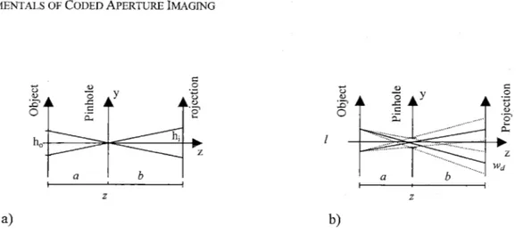
CHAPTER 2 FUNDAMENTALS OF CODED APERTURE IMAGING 2.1 THE PINHOLE CAMERA

2.2 ENCODING THE SIGNAL: OBJECT PROJECTION

6

3

5

6

10

12

13

17

19

19

21

22

25

26

27

29

29

31

2.3 DECODING: COMPUTER POST-PROCESSING 35

2.4 CODED APERTURE FAMILIES 38

2.5 CODED APERTURE CAMERA GEOMETRIES 58

2.6 FIELD OF VIEW AND RESOLUTION 60

2.7 DECODING TECHNIQUES 66

2.8 DEPTH OF FOCUS AND 3D LAMINOGRAPHY 72

PART I: METHODS, THEORETICAL ADVANCEMENTS AND EXPERIMENTAL RESULTS

75

CHAPTER 3 SIMULATION TOOLS: COMPUTER CODES AND OPTICAL BENCH 77

3.1 THE SIEMENS E-CAM 77

3.2 THE SIMULATION CODE 78

3.3 THE OPTICAL SIMULATOR 85

3.4 VALIDATION WITH E-CAM DATA 90

CHAPTER 4 THE SIGNAL-TO-NOISE RATIO IN CODED APERTURE IMAGING 93

4.1 AN INTUITIVE SUMMARY OF THE PROBLEM 94

4.2 SNR DEFINITION AND CHOICE OF THE DECODING COEFFICIENTS 95

4.3 THE SIGNAL-TO-NOISE RATIO OF DIFFERENT CODED APERTURES

103

4.4 COMPARING THE SNR PERFORMANCE OF DIFFERENT ARRAYS

111

4.5 DEPENDENCE OF THE VARIANCE ON OTHER SOURCES

115

4.6 SIMULATIONS

117

4.7 OBSERVATION ON THE RELATION BETWEEN SNR AND SENSITIVITY

117

CHAPTER

5

ARTIFACT THEORY 119

5.1 MASK TRANSMISSION

119

5.2 SAMPLING

120

5.3 ROTATIONAL MISALIGNMENT

123

5.4 NEAR-FIELD ARTIFACTS

123

5.5 VERIFYING THE NEAR-FIELD ARTIFACT THEORY

133

5.6 NEAR-FIELD ARTIFACT REDUCTION

135

5.7 EXPERIMENTAL RESULTS

136

5.8 MASK THICKNESS ARTIFACTS

136

5.9

SUMMARY

137

CHAPTER 6 DESIGN AND FABRICATION OF A CODED APERTURE: EXPERIMENTAL

RESULTS 141 6.1 MASK DESIGN

141

6.2 EXPERIMENTAL RESULTS

147

6.3 ELECTRONIC FOCUSING 150 6.4 IN VIVO EXPERIMENTS

152

6.5 SUMMARY

156

PART III: ADVANCED TOPICS AND FUTURE DEVELOPMENTS

159

CHAPTER 7 ADVANCED MASK DESIGN 161

7.1 RESOLUTION IN A REAL DETECTOR

161

7.2 CHOOSING A CONFIGURATION

170

7.3 THE DESIGN OF AN OPTIMAL RESOLUTION MASK

171

7.4 AN IMPROVED FIGURE OF MERIT 174

7.5 EXPERIMENTAL RESULTS: ...1N

182

7.6 SUMMARY

184

CHAPTER 8 EXTENSIONS AND FUTURE WORK 187

81 EXPERIMENTS WITH THE CURRENT MASK 187

8.2 EXTENSION TO HIGHER ENERGY 188

8.3 ARTIFACT REDUCTION 191

8.4 THREE-DIMENSIONAL IMAGING 191

CHAPTER 9 APPLICATION TO CAFNA 197

9.1 BASIC PRINCIPLES OF CAFNA 197

9.2 THE BASICS OF FAST NEUTRON ANALYSIS 198

9.3 A

ID

CARBON IMAGE 211

9.4 DESIGN OF A CODE APERTURE FOR CAFNA 214 9.5 SUMMARY 215 CHAPTER 10 CONCLUSIONS 217

APPENDICES

221

BIBLIOGRAPHY

251

9

CAPITAL BOLDFACE indicates a discrete 2d function or matrix.

Lowercase boldface indicates a Id array.

CAPITAL ITALIC indicates a continuous 2d function or a scalar variable.

Lowercase italic indicates a continuous I d function or a scalar variable.

definition

x:

correlation: H(5)

=

F(i)

x

G()

=

JJF(5)G(9+

-d

2,

0:

correlation (periodic): H(Q)= F(1i) 0 G(i)

J=JF()G( D h)d

2

i

*:

convolution: H(Q)

=

F(i) * G(i)

=JF(X)G( -i)d%2

0:

sum modulo p

Q.

cyclic difference set

9:

Fourier transform operator

3:

Inverse Fourier transform operator

91:

reflection operator

A:

aperture transmission function

A': projection of the aperture on the detector

AT:

finely sampled aperture array

AF: finely sampled aperture array, 6 decoding

G:

decoding function

GF:

finely sampled decoding array

GFS: finely sampled decoding array, 6

decoding

GO:

sampled decoding array resulting in no

sidelobes

H:

rect function

N:

noise distribution

0:

object intensity distribution

0': pinhole image of an object

0:

object estimate

R:

recorded data

Y:

concentration parameter

a:

b:

object-to-mask distance

mask-to-detector distance

10

Cr: quadratic residues modulo r.

dd: detector size

d,,: mask size

e: NTHT array parameter

f:

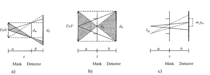
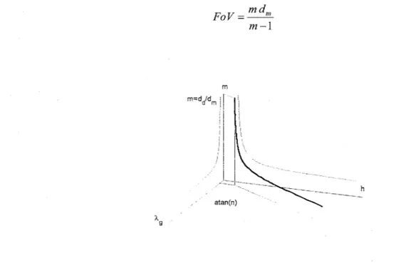
illumination fractions

FoM: figure of merit

Fo V: field of view (fully-coded)

M: magnification coefficient (coded aperture camera)

np: magnification coefficient (pinhole camera)

n: number of mask pixels (side); integer

pd: detector pixel size p,,: mask pixel size

r: radius

r : position vector

t: mask transmission

t,: thickness of one mask layer

x, y: coordinates w,.: pinhole width

M:

sidelobe height

N:

total number of open holes in a mask

NT: total number of positions in a mask

p,: mask pixel size S,,: shape of mask pixels S: shape of detector pixels

S',M: shape of the projection of a mask hole on the detector

z: object-to-mask distance

U: sampling parameter; incidence angle 5: Dirac delta function

5(i,j): Dirac delta function

AS:

angular field of view

0:

incidence angle

Xg:

geometric resolution

k,:

system resolution

p:

attenuation coefficient; mean value

p:

array open fraction (density)

CY:

standard deviation

4:

noise parameter

X:

parameter for the calculation of the effects

of the intrinsic PSF on resolution

Q:

solid angle

Also see section 4.2 for a description of the

symbols involved in SNR calculations.

LIST OF ACRONYMS

CAFNA: Coded Aperture Fast Neutron Analysis

FCFV:

Fully Coded Field of View

FFT:

Fast Fourier Transform

FNA:

Fast Neutron Analysis

FWHM: Full Width at Half Maximum

FZP:

Fresnel Zone Plate

MURA: Modified Uniformly Redundant Array

NRA:

Non Redundant Array

NTHT:

No-Two-Holes-Touching

PCFV:

Partially Coded Field of View

PSF:

Point Spread Function

SNR:

Signal-to-Noise Ratio

URA:

Uniformly Redundant Arrays

The original motivation for our research group to study coded apertures was the development of a

non-intrusive bulk inspection system, CAFNA (Coded Aperture Fast Neutron Analysis), which has been

under development at MIT for a number of years. CAFNA is the combination of coded aperture imaging

with Fast Neutron Analysis (FNA), an established bulk analysis technique based on the detection of

y-rays generated by inelastic scattering of fast (>1 MeV) neutrons. Since the energy of the photons emitted

is specific to the isotopes present in the inspection volume, FNA is sensitive to the isotopic composition

of materials. Information on the relative and absolute amount of common elements such as carbon,

oxygen and nitrogen can uniquely identify a number of materials ([1], [2]), hence the interest in the

technique for security applications (explosive detection in luggage or cargoes) and contraband detection.

Since the cross sections and solid angles involved in FNA of a volume as large as a cargo container

typically lead to poor statistics, it is imperative to make optimal use of the photons obtained. The idea at

behind CAFNA is to form an image of the spatial distribution of the y-rays generated in FNA by using a

coded aperture in place of inefficient image-forming devices like collimators and pinholes.

The design of a CAFNA system requires work on two system components: a position and

energy-sensitive y-ray detector and the coded aperture. Of course the two problems are interdependent, the design

of the detector depending on the design of the coded aperture and vice-versa. Both detector and aperture

need significant development, but, while the considerations involved in the design of the detector can rely

on a well-established body of knowledge, the design strategy of the coded aperture was largely uncharted

territory to us. To get an approximate idea of the requirements on the detector we needed to tackle this

latter problem first.

The complexity and size of a system such as CAFNA not only demanded theoretical

investigation, but also verification by simulation and experiment, which requires use of a

y-ray

detector.

To this end, we needed to concentrate momentarily on a problem for which a fully-developed 7-ray

position-sensitive detector is already available. This is the case of the Anger (or gamma) camera in

Nuclear Medicine, so we started looking into the problem of taking a 7-ray picture of a thyroid (a classic

test object in the field) with maximum resolution and Signal-to-Noise Ratio (SNR). At the beginning, the

study focused on the determination of basic imaging parameters of the coded aperture camera (the

combination of a coded aperture with a detector) such as field of view and resolution. Simulations

confirmed the predictions of the theoretical analysis, but also showed that other factors, in particular the object-to-detector distance, play an important role in the imaging process. This was not surprising, because we were aware that coded aperture imaging was originally developed for a very different application, X-ray space telescopes. The geometry of this case (a far-field problem, because the object can be considered very far from both coded aperture and detector) is radically different from that of our case (a near-field problem, because, for counting efficiency reasons, the object must be kept as close as possible to coded aperture and detector). In particular, all the apertures that in far-field ensure artifact-free

imaging deviate significantly from ideality when used in near-field. The goal of devising a rational design

procedure for the coded aperture was now expanding to include near-field artifact reduction. A second finding of the simulations was that, among the many apertures that provide ideal far-field imaging, some

families have a SNR significantly superior to others, which opened yet another question, that of finding

the optimal aperture family. This thesis describes the theoretical analysis developed to address these

problems, the supporting simulations and experimental confirmation of the theory, and the solutions implemented in the design of a prototype coded aperture to answer all challenges in a rational and practical way.

There are two main results of this work. The first is the experimental demonstration of the

feasibility of near-field artifact-free imaging over small fields of view. The high SNR achieved despite

the high resolution (about 3 times better than achieved by state-of-the-art collimator and pinhole systems)

is very promising for immediate application in routine small-animal laboratory planar studies. The design

ideas presented in this thesis allows one to continue the development of a coded aperture camera for Nuclear Medicine along several lines. First, preliminary studies show that sub-millimeter resolution can

be reached while retaining acceptable SNR. Even more interesting is the case of isotopes emitting high

energy y-rays, which, penetrating collimator septa, are very difficult to image with conventional methods.

Second, the experience gained in the Nuclear Medicine study is the best validation of ideas and

procedures general enough to be applied to CAFNA. A better understanding of the performance of coded

apertures has allowed us to estimate the requirements of a satisfactory y-ray detector. In particular, a

prototype detector under development at MIT already seems to provide sufficient energy and position

resolution. Its limit was rather found in its size, currently limited to an 8x8 array of 10 x 10 cm detectors, but can be easily overcome with translations in this experimental phase and by simply building a larger array in a full-scale system.

The results of the Nuclear Medicine application have met considerable interest in the medical arena, for both animal and human studies. The development of new pharmaceuticals typically passes through small animal studies whose aim is to identify if the compound is actually metabolized as

expected. Given the dimensions of the animals, resolution is key in these studies. With the 6-mm

resolution characteristic of current methods it is very hard to identify parts of organs often smaller than a

centimeter. Sub-millimeter resolution would provide researchers with a tool more practical than

autoradiography techniques, which require painstaking surgical procedures and sacrifice of the animal,

precluding time-dependent studies. Resolution is also of great interest in pediatric imaging, where

reduced dimensions pose a challenge to current instrumentation, and in adult studies, such as breast

imaging. This application is particularly suited to coded aperture imaging because it requires that a hot

spot be located on a colder background. In this case better resolution can lead to all the benefits of an

earlier diagnosis.

Given this potential, the investigation of coded apertures for nuclear medicine has become an

independent project which will be hopefully continued in the future.

The goal of this Chapter is to put this thesis in context and introduce some problems of coded

aperture imaging, so that the thesis outline can be discussed in some detail. Accordingly, only a broad

overview is provided of questions that are going to be discussed in the next Chapters, to which rigor is

postponed for clarity and brevity. Reviews of coded aperture imaging basics can be found in ref. [3]-[6].

1.1

The classic methods of 2d imaging

An image is a mapping over space of some distribution, in our case that of a photon emitter. At

the energies of our interest (140 keV

-

10.8 MeV)

1

wavelengths are small (8.9 pm

-

115 fin), so that

diffraction can be neglected and geometric optics used with excellent approximation. Placing a position

sensitive detector directly before the emitting object (source) is not enough to generate an image because

any photon detected (event) could be due to any part of the source (Figure

1.1a).

In this sense, no spatial

information is obtained and it is impossible to produce an image. An imaging system must associate

o-S

Source Pinhole Detector

b)

*---Source

c)

Collimator/Detector

Figure 1.1: a) if no imaging system is present, a count collected at the detector can not be traced back to any specific part of the source. A pinhole (b) and a collimator (c) establish a one-to-one correspondence between detector and object. With a geometrical construction one can associate each detected event with an emission location.

140 keV is the energy of the

y-rays

from the de-excitation of 99mTc, used in the great majority of Nuclear Medicine exams. 10.8 MeV is the energy of a thermal capture event on 14N, a reaction used in explosive detection

systems based on thermal neutrons. Source

a)

events with a place of emission.

The simplest imaging device is the "pinhole", a slab of material opaque to radiation in which is poked an infinitely small (ideally dimensionless) hole. Since every event must have come from the object through the pinhole, along a straight line (Figure 1.1b), every point of the detector represents a point of the source and an image is formed. By inspection, the photon distribution recorded at the detector is an

inverted picture of the object. A second system is the parallel-hole collimator, an array of infinitely small

little tubes, whose walls are opaque to radiation, typically of hexagonal or circular section, placed side by side until the detector is covered. In this case, photons must have come from a line perpendicular to the

detector (Figure 1.1c), which identifies the place of emission. The image is directly the photon

distribution recorded by the detector.

Ideal pinholes and collimators share the property of realizing a one-to-one correspondence between object and image. Also, in both cases, for a given source, only photons traveling in one direction are collected. Lens systems also work with the same idea of one-to-one correspondence but, unlike

pinholes and collimators, bend the path of incoming photons. This means that a point of the source can

Total source counts 350k

Total source counts: 35M Totat source counts: 35M

a)

b)

Figure 1.2: a) resolution

loss

when an ideal pinhole is enlarged to increase throughput. b) intuitive visualization of

the trade-off between noise and resolution for pinhole and collimator imagers. Three pictures of the original object

(top left) were simulated for constant exposure time. The ideal pinhole was

1

xl

image-pixels wide (1:1

magnification). The

image

is very noisy (top right). To obtain better statistics one can widen the pinhole to l0x 10

image pixels and collect 100 times more counts. This does improve the signal in the image (bottom

left)

but also

blurs it. In a half-open

1

5x1 5 coded aperture there are approximately 100 lxi pinholes: hopefully, this yields the

same signal advantage of the

larger

pinhole while preserving resolution (bottom right).

In

Chapter 4 we will see that

this argument holds for a point-like source only. For images as complex as the one chosen here, depending

on

its

statistical details, there may be no SNR advantage in using a coded aperture.

contribute a whole cone of different directions to the image, with great advantage for the SNR.

Unfortunately, photons of the energies of our interest can not be bent by refraction optics. Bragg diffraction mirrors used in space telescopes work well up to 15 keV ([3]), but further extension requires sophisticated manufacturing techniques and does not exceed 80 keV.

In theory, the resolution provided by an ideal pinhole (i.e. a dimensionless point) is perfect. An intuitive argument is that two point sources arbitrarily close in the object will always show separated on the detector2. However, this comes at the price of no counts at all, because the area of the ideal pinhole is zero and the photon flux through it must be zero as well. This is also true of collimators, but not of lenses, which offer a finite area to the incoming flux, but, again, do not work at the energies of our interest. Real

pinholes, however, must have a finite size. This allows some photons to pass, which does increase the

SNR, but does not come completely to our rescue. Figure 1.2a shows that if two point sources are close enough, their projections on the detector, which would be distinct in the case of an ideal pinhole, are not separated. Resolution must have decreased. Another way of looking at the same issue is to recognize that the larger pinhole realizes only an "approximate" one-to-one correspondence. For a complex object, resolution loss means a blurred image. This is shown pictorially in the example of Figure 1.2b, where the ideal pinhole (in this example a very small hole of finite size) is compared to a real one.

In conclusion, the pinhole (or collimator) hole size can not be increased indefinitely to increase

efficiency because some resolution limit will be reached. In typical collimator systems only 0.1% or less of the emitted photons are counted, giving a noisy image unless a long exposure time is used or lower resolution accepted for a constant exposure time.

1.2

Why a coded aperture?

Coded apertures try to achieve the resolution of small pinholes while maintaining a high signal throughput. The basic idea is to overcome photon shortage by opening many small pinholes instead of a

larger one. These pinholes are placed in specially designed arrays called patterns. The aperture (or mask)

is the physical realization of a pattern. The mask forms with the detector the coded aperture camera.

2 Since here we are concerned with the properties of the imaging optics, not with the system as a whole, an ideal (perfect resolution) detector is assumed. A complete discussion of the resolution of a coded aperture camera is given in sections 2.6 and 7.1.

1.3

Coded aperture imaging in a nutshell

Since the number of photons passing through a pinhole of the coded aperture is independent of photons passing through all other pinholes, each pinhole is independent of the others. The projection of the object through the mask can be decomposed in the sum of contributions from each pinhole. From the discussion of section 1.1, a pinhole casts on the detector an inverted image of the object, which superimposes to projections from other pinholes (Figure 1.3a). The counts collected at the detector are,

then, the superposition of many shifted copies of the object. In a far-field approximation, i.e. when the

object is sufficiently far from mask and detector, the projection process follows the equation:

O

xA=R

(1.1)

where 0 is the irradiance (number of photons emitted per unit area) of the object, A the transmission of the coded aperture (a function ranging from 0 for complete opacity to

1

for complete transparency), R the

counts recorded by the detector and x indicates non-periodic correlation. A rigorous definition of the

far-field approximation is given in Chapter 5, where eq. (1.1) is derived as a particular case of a more general

formulation.

As the pinholes can be several hundreds, R does not resemble 0 in any immediate way. An

alternative way of looking at the same process is to say that a point in the image is not represented on the

detector by a point, but rather by a pattern of points. This is the mask itself, as follows from eq. (1.1),

when 0 is replaced with Dirac's delta function 6:

R=SxA=A

(1.2)

Therefore, each point source is present in the projection not as a point but as a known pattern.

Original M ask

URA

CAMERA 2

0 20 40 60 0 5 10

Projection Fourier Reconstruction

ECONSTRUCTED APERTUREECDDTMAGE P"CT*W W1PUTER'01

30

₃

DECODING

a)

PROCEDURE

b)

a10

20 2n4600

Figure 1.3: a) pictorial summary of a coded aperture camera concept (here indicated with a URA camera). Adapted from [6]. b) a sample of the process from the object, through the mask, to projection and reconstruction.

Different point sources are characterized by the pattern shift. In this sense the signal from the source is encoded. The first consequence is that a point source is not counted once, but once for every pinhole of the coded aperture, which is expected to increase the counting statistics and, consequently, the SNR. The second consequence is that at each detector point is present information about many points of the source: in this sense information is multiplexed. The third consequence is that the recorded pattern R must be decoded to obtain an image. In intuitive terms, R must be scanned looking for known patterns which must be replaced with the point source that cast them. This is the same as separating the overlapped copies and is done by an operation known in signal processing as "matched filtering" ([5]). The technique prescribes to take the correlation of the collected data with the known pattern, in our case A. In a more general case in a pattern may be sought not through the pattern itself, but through an associated decoding pattern (or decoding array) G such that:

A®G=S

(1.3)

where 0 indicates periodic correlation, the matched filtering process is:

ROG

(1.4)

The result of this operation is to produce a perfect copy of the object 0. In fact, given the linearity of correlation operations and eq. (1.1) one can write (using Appendix A.3):

O =R0G=(0xA)®G= O* (AOG)

(1.5)

where

0

is by definition the estimate of the object or reconstructed image. This chain of equalities shows that the output of the imaging system is not directly the object but, as in all linear systems, a convolution of the object with a kernel, in this case A 0 G. The convolution kernel is also called the Point Spread Function (PSF), which is the imaging analogue of the Pulse Response Function of electrical circuits. With

this definition, eq. (1.5) becomes:

0=0

* PSF

(1.6)

The name Point Spread Function comes from the fact that the PSF is the image produced in

response to a point source. In fact if 0 = 6:

which means that the PSF describes the imperfections that cause a system not to reconstruct a point with a point, but to spread it over a certain area. The PSF summarizes the behavior of the imaging system because the output of the imager can be predicted from knowledge of the input (the object) and the PSF alone, via eq. (1.6). Its importance is enormous both in theory and in practice. From eq. (1.5) and (1.6), in coded aperture imaging:

PSF

=

A 0 G

(1.8)

Fortunately A and G are both in the hands of the designer. Furthermore, considerable literature is

dedicated to the generation of pairs of A and G satisfying the constraint of eq. (1.3). Such pairs are said to

have perfect imaging properties. In fact, substitution of eq. (1.3) in eq. (1.8) and then in eq. (1.6) gives:

0=0 * 6Z=0

(1.9)

which means that if the PSF is a 6 function the reconstruction is perfect. This should not be surprising, because in this case a point in the object corresponds to a point, and not a blur, in the image.

In conclusion, coded aperture imaging can produce a perfect copy of the object. It is a two step

process: the first is physical, the projection of the source through the aperture; the second is

computational, decoding. The motivation to go through this complication is the potential of achieving a

higher SNR. Chapter 4 is dedicated to quantifying this potential and understanding the hypothesis under

which it is actually present.

Of course, the result of ideal reconstruction is due to a number of hypotheses. The first, and most

relevant, is that eq. (1.1) holds only in the above-mentioned far-field approximation, which is the implicit

starting point of all coded aperture literature. This approximation does hold in most literature

applications, especially the early ones, which developed the basic ideas of coded aperture imaging in the

context of space applications. However, in Nuclear Medicine, the concern is to collect the maximum number of photons, and the detector must be placed as close as possible to the source. In typical cases, the

far-field approximation breaks down, but little attention to this is found in published works. Chapter 5 is

dedicated to the examination of the consequences of using methods developed for far-field applications in

a near-field geometry and the development of suitable remedies.

The second major hypothesis is that detector and mask be ideal. As for the former, a typical state-of-the-art Anger camera provides a 3 .7-mm-FWHM (Full Width at Half Maximum) PSF at the center of the crystal. This means that an infinitely narrow beam is seen not as a point but as a blur reaching half of its peak value only outside a diameter of 3.7 mm. This figure gives a first idea of the resolution that can

be reached with such a system, but it has to be combined with a second factor. In fact, eq. (1.3) holds in this exact form only for an aperture with dimensionless pinholes. Real pinholes and collimators have a finite size, which further degrades resolution. As an example, the Ultra-High-Resolution collimator supplied by Siemens for use with its E-Cam gamma-camera has a hole diameter of 1.16 mm and is capable of a system resolution of 6.3 mm for 99'Tc at 10 cm. This collimator, however, has the low sensitivity (counts per unit activity in the source) of 100 cpm / pCi at 10 cm. For comparison, a High-Sensitivity collimator (1063 cpm / pCi at 10 cm) has a resolution of 14.6 mm at 10 cm. In Chapter 7 is provided a thorough description of how all these factors were combined in the determination of the resolution of a coded aperture camera and how the limits for the achievable resolution were investigated.

1.4

Coded aperture history

Coded aperture techniques were first proposed in 1961 by Mertz and Young ([7]). The aperture they proposed was the Fresnel Zone Plate (FZP), in theory a circularly-symmetric mask having transmission:

cos (r

2

); 0 : r ;+c00

(1.10)

where r is the radius from the center of symmetry. This pattern was inspired by holography, where it is used for its property of refocusing coherent light in a focal point. This characteristic can be used to decode the projection. In early experiments the projection was recorded on a film, which was developed and then exposed to coherent light of wavelength comparable to the size of the projected pattern. Since each projected zone plate is refocused in a point, the image is decoded. Note that while the projection is cast by X or y-rays, coherent radiation of optical wavelength is used in decoding, which was an optical

A

_(b)

Figure 1.4: theoretical (a) and practical (b) Fresnel Zone Plate. The latter is non-ideal because transmission is either total or null (instead of being continuously modulated) and because the plate is not infinite but stops after a few

circles.

procedure ([6]).

The advent of fast digital computers made it possible to exploit a second nice characteristic of the FZP: the auto-correlation of an FZP is a

a

function ([3]), so the decoding method of section 1.3 can also be used. However, perfect imaging properties hold only if the plate is infinite and has a continuously varying transmission. Since this entails considerable fabrication difficulties, in real applications the FZP must be approximated with a finite series of concentric circles of radius:

r,, = r-fJ,

n =,

2

,

3

... ,nm

(1.11)

where the annuli are alternatively totally opaque and transparent (Figure 1.4). A particular case is that of the annulus, where a single open ring is used. These approximations cause significant deviation from a 6

function, even if more general formulations of eq. (1.11) are used ([8]). This, however, did not stop early

experiments. Despite having been proposed for space applications, the first actual demonstration of FZP

imaging was a study of a thyroid phantom ([9]). Fabrication difficulties, with the problems associated

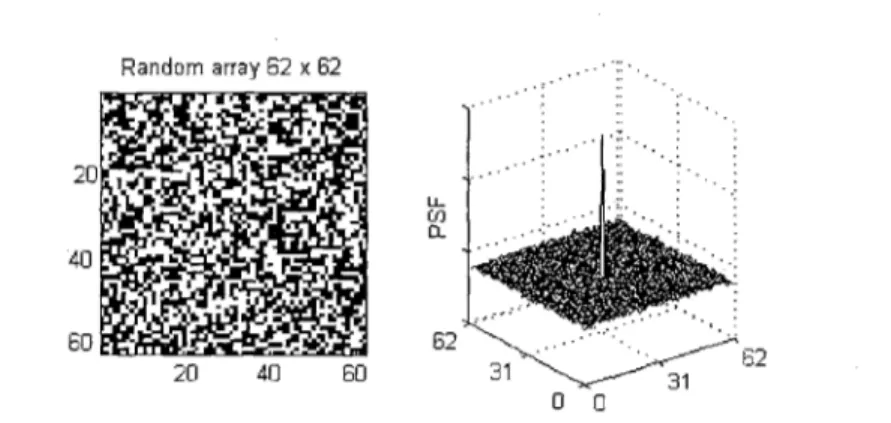
with optical decoding, made the technique impractical.

The advent of more manageable apertures gave new momentum to the field. In 1968, Dicke and

Ables independently pointed out that a square arrangement of randomly distributed square openings (a

random array) has reasonable self-correlation properties ([10], [11]). Unfortunately, just like the FZP, a

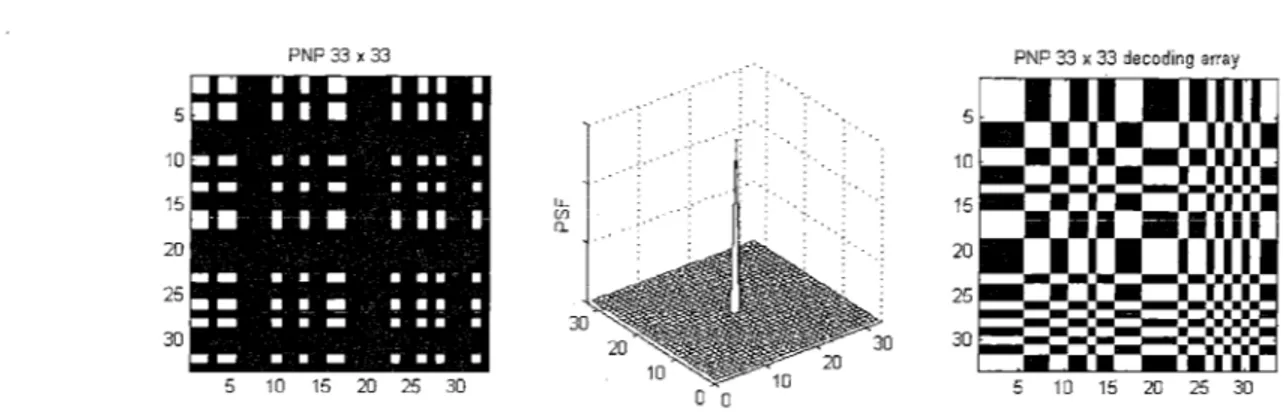
random aperture provides an ideal PSF only if it is infinite. In 1971 the Non Redundant Arrays (NRAs, [12]) were proposed. These arrays are compact but have ideal properties only on a small field of view and contain a small number of holes, which prevents great improvements in the SNR. The difficulty was

overcome in 1978, when Fenimore and Cannon introduced the rectangular Uniformly Redundant Arrays

(URAs, [13]), which have an ideal PSF and are finite. A decade later URAs were followed by the

Modified URAs (MURAs), which have the additional convenience of being square ([14]). Meanwhile, a

number of other apertures were discovered. They are described in section 2.4.

1.5

Applications of coded apertures

Applications of coded apertures have been, for the vast majority, in astronomy. A number of examples can be found in ref. [3]. This is due to two reasons. The first has to do with the appearance of the object (in astronomy a number of isolated bright spots, the stars) and the detector high-background environment, often an orbiting satellite or a balloon-borne telescope. As we shall see, it is in these conditions that coded apertures provide the largest SNR advantages over pinholes and collimators. The

second reason is that star imaging is a perfect example of far-field imaging, a condition not affected by artifacts.

Other fields of application are nuclear medicine ([9], [l5]-[18]), nuclear fusion ([19], [20]), industrial imaging, e.g. clean-up and decommissioning of nuclear sites ([21]), contraband detection ([22]),

chemical spectroscopy and optical image processing ([3]).

1.6

Thesis outline

The thesis is divided in three parts. As the reader will have found out by now, Part I provides context and a general overview. The second Chapter is a more detailed presentation of coded aperture imaging. An analysis of the imaging geometry is presented with the goal of deriving fundamental relations among basic parameters such as field of view and resolution. For comparison reasons, the case of the pinhole is also briefly summarized. Extensive details on the options available for the aperture and decoding pattern are provided. Listing all pattern families and generation rules may seem tedious and not original, but the goal was to provide some order in information otherwise scattered in a number of papers. Furthermore, a reasonably comprehensive knowledge of patterns is very useful in understanding SNR and artifact reduction problems. Some considerations on the 3d properties of coded apertures close the Chapter.

Part II of the thesis is its original core. It discusses the simulation and theoretical tools used in the investigation, how they were used in the design and construction of a prototype aperture and the experimental results obtained.

Simulation has played a fundamental role in this project to the point that it is not unfair to say its results directed the work. Since some aspects of simulation are not trivial, Chapter 3 describes the simulation code. In this Chapter is also included a description of the optical simulator that provided the first link between the computational and the real world, supporting the credibility of computer calculations.

Chapters 4 and 5 concern, respectively, the SNR and artifact reduction. A major problem was finding a rational procedure to design the coded aperture. For example, from literature are known several families of pairs (A, G), and, within each family, patterns of many different sizes. Since all families and patterns provide ideal far-field imaging, the problem was to find some other criterion that made a family preferable to others. To answer this question, Chapter 4 looks closely at the SNR of coded aperture families. One of the conclusions is that coded apertures do not always provide an advantage over a pinhole or collimator system. In particular, a coded aperture is advantageous for sparse objects (a result

well-known in the literature), i.e. objects for which the activity is concentrated in a relatively small part (on the order of 10% or less) of the field of view, unless a very high background is present. A less-known result is that low-throughput apertures do not always provide better performance for sparse objects, a

statement that has led some researchers to erroneously propose some aperture families as optimal for medical applications. Finally, investigations in the literature have considered the ideal system: for instance, the area around mask holes is perfectly opaque and far-field geometry is assumed. In the analysis of the SNR partial mask transparency is introduced because, while it does not introduce any artifacts, it does reduce the SNR. Results extend and correct some of those previously published and will be later applied to the determination of mask thickness and in the investigation of higher energy isotopes.

In Chapter 5 several other non-idealities are presented and their impact on the final image

described. These are mainly related to how the detector samples the projected pattern, but the most

interesting for planar imaging are those due to near-field geometry and mask thickness. The far-field approximation is derived as a particular case of a more general mathematical framework capable of predicting near-field artifacts, which are described, classified and compared to published results. On these bases, some remedies are proposed and their effectiveness tested with computational simulations. The Chapter closes with a description of the origin of thickness artifacts.

The pairs (A, G) are found in literature as dimensionless 2d arrays of numbers. The question of

finding the physical dimensions to fabricate a pattern into a mask is closely related to that of finding the

field of view and the resolution of a coded aperture camera. Chapter 6 tackles the problem in a systematic

way by applying to the design of a coded aperture the concepts developed in previous chapters. The reason for every value of a mask specification is explained. The mask designed was actually built and experimental results are presented.

Part III contains advanced topics and extensions of the work presented in Part II. Chapter 7

revisits the resolution of the prototype mask to include the effect of detector sampling and intrinsic PSF.

After different detector setups are discussed, the characteristics of an advanced mask design, capable of

sub-millimeter resolution, are derived. Since the ultimate limit on resolution is found to be mask thickness, a method for an accurate determination of optimal thickness is developed.

Chapter 8 is about future work that can be done with the prototype mask, the bases for the imaging of higher-energy isotopes and the general issues involved in 3d coded aperture imaging.

Finally, Chapter 9 introduces fast neutron analysis and presents experimental results which provide insight on issues, such as background and noise, likely to play a prominent role in the design of a

This Chapter explores the fundamentals of coded aperture imaging more in depth. First, the

pinhole camera gives an opportunity to introduce at an intuitive level many ideas useful for what follows.

Different aperture families, code aperture camera geometries and decoding strategies are then presented

along with many different families of apertures. A few considerations on elementary three-dimensional

properties of coded aperture imaging close the Chapter.

A basic exposition of coded aperture imaging that also provides historical background can be

found in ref. [6]. Ref. [13] is more technical and is probably the most referenced paper in the field.

2.1

The pinhole camera

The photon distribution recorded at the detector of a pinhole camera follows from the one-to-one

correspondence established between object and detector. With the definitions of Figure 2.1, the photon

distribution at a generic detector position R (xi, y,), must be due to the point source at (x0, y,) only, to

whose irradiance 0 (xo, yo) must be proportional:

R(x,y,)oc O(x, y)

(2.1)

Defining the vectors:

1i =(x, y

)

and

t= (x, yo)

(2.2)

which, because the ray going from Ft to i must pass through the pinhole, are related by:

a

il =b-,(2.3)

eq. (2.1) becomes:

y1 x13

C) )1__77

-Yi

b

Figure 2. 1: pinhole camera geometry.

This relationship shows that the projection through the pinhole is a copy of the object, inverted

(because of the minus) and rescaled. Since a and b can be any positive number, the rescaling constant can be any positive number. If a> b, i.e. the pinhole is closer to the detector than to the object, the object

appears minified, while for a < b, the object is magnified. From Figure 2.2a one can verify that the ratio

of the projected object size to the original is (neglecting the inversion):

hiyb

hi- b-=M P(2.5)

ha b

which demonstrates that the rescaling coefficient is the magnification coefficient of the pinhole m,.

If ha is set equal to the size of the detector, ds, the size of the field of view of the pinhole, i.e. the

set of points in the plane of the object that can be imaged, is obtained:

Fo V = (2.6)

MP

In the case of the ideal pinhole, resolution is, of course, perfect. If the pinhole had a finite width

w,,, each point would cast an image of size:

Wd - a+ b Wll=(+ MP ) W. (2.7)

a

If the resolution of the system is defined as the minimum distance between two pot i in the plane of the object such that their projections are separated in the image, from Figure 2.2b and simple geoetry:

a) b)

Fiue22 0)Dtriaino h pinol manfcto ofain )Dtriaino ihl eouin

A'6 Y 9 o .D .r-h o...

a1

1= /Z .. . ... a + - , ciw 28 b m

a)

b)

Figure 2.2: a) Determination of the pinhole magnification coefficient b) Determination of pinhole resolution.

I

W",(2.8)

a

W

= 1

b

_M

With this definition of resolution, low values indicate good resolution. This clarified, this

equation shows that the best case is that of infinite magnification and that resolution is limited by the size

of the pinhole. It is interesting to note that while resolution improves for increasing magnification, the

field of view shrinks. The ratio of the two is:

FoV

dd

(2.9)

1

(1+m)w,,

This ratio could be taken as a figure of merit for an imager, which ideally should have the widest possible field of view and, at the same time, the best possible resolution. The maximum value is dd / w,,

and is obtained for m,

->

oo. As magnification increases, resolution improves but eventually reaches the

asymptote w,, while the field of view decreases indefinitely until the figure of merit vanishes.

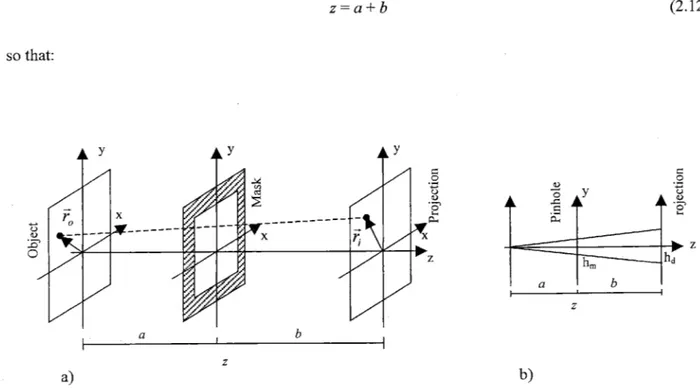
2.2

Encoding the signal: object projection

Chapter

1

showed that coded aperture imaging is a two step process. The first step, encoding, is the physical process of projection of the object, through the mask, onto the detector. Since at the energies of interest geometric optics is applicable, it is possible to calculate the projection from aperture and object

with a purely geometrical argument. With the definitions of Chapter 1 and Figure 2.3a, the photon

distribution R recorded at the detector position , and due to the point source at

F%

must be proportional

to the irradiance

0

(4),

modulated by the transmission of the mask A evaluated at the point of

intersection with the ray going from 1, to

4r:

R()

o0(F)AK,

+

P

a

z)

(2.10)

To simplify construction, A is almost always considered a two-valued function. It is also very

often thought as a grid of square elements, so that it can be represented with a matrix whose elements are

Is and Os (respectively, holes and opaque elements). To obtain the total recorded photon distribution, it is

sufficient to repeat this argument for all point sources and add all the results, i.e. integrate over the object

plane:

R(4)oc

JO(F,)AL4,

+

"-

a d20

K o

z

(2.11)

Here the assumption that the detector responds linearly is made, i.e. the response to the

simultaneous exposition to several sources is equal to the sum of the responses obtained from the sources

taken one at a time. By definition:

za+b

A

(2.12)

so that:

A

4-4

rVrt

'C

V

a

A'

a 0 C.) C) 0

V

_'C z

~5y

hm hd a b

-4

T)

b

z

a)

b)

Figure 2.3: a) projection geometry. b) calculation of the magnification coefficient of the mask

H i :7r I

W-LOA If

A

z-R(Fc

IO(,)Ara ;b"d20

(2.13)

which, with:

b

b

=--r,,(2.14)

a becomes:

R(5)a c

JJO(=ffh)A<Y

)jd2

(2.15)

From its definition,

4'

is the point that would be associated to

F

in-a pinhole imager, i.e. it is the point of the detector aligned with , and the mask center. Two more definitions will help cast this equation in a more meaningful form:

'

r-0

F

and

A'()=

A

f <

(2.16a-b)

0' is a scaled and inverted version of 0. The scaling coefficient is the same as the magnification

coefficient of a pinhole camera (see eq. (2.5)). In other words, 0' is a pinhole image of the object (eq. (2.4)). Similarly, A' is a scaled (but not inverted) version of A. The scaling coefficient makes A' larger than A. Figure 2.3b helps in the calculation of the ratio of the size of the mask projection to the size of the mask itself:

h Z

--- = - Z(2.17)

h,,

a

which is the scaling coefficient of definition 2.16b. The magnification of A' is due to the projection of

the mask pattern on the detector. Substitution of eq. (2.16a-b) in eq. (2.15) gives:

RQ(j;) cc Jo'(4 ' )A'Q

7i

) d

0'A'(2.18)

which shows that the projection process is described by the convolution

3

of the pinhole image of the

object

0'

with the projection of the mask pattern A'. A physical interpretation of this equation is that the

projection is the sum of magnified mask patterns, each shifted according to the location

4

of the point

source casting the shadow and weighted according to its irradiance.

An alternative interpretation is obtained exploiting the commutative property of convolution:

R=O'*A'=

A'*O'=

JJA'Q

,',)0'(i

-,|,)d

2i,|

(2.19)

where

4

is a dummy variable spanning the detector. In this form the projection is the sum of equal

pinhole images of the object, shifted and weighted according to various positions in the mask. From

Chapter 1 we know that the aperture is in practice a collection of N pinholes. Assuming ideal pinholes, A

can be written as a sum of shifted 6 functions:

A(F,,)

=

Z6

Q,,

-1F,)

(2.20)

n=1,2,...N

where ,, is a generic position on the mask plane and F,,,, the position of the nib pinhole on the plane. The

projection of A on the detector is:

A'(,|%)=

Z6(F,

-t,

(2.21)

n=1,2,.. N

which can be substituted in eq. (2.19) to get:

R

=

f

Z

(,|

-rf| )O'(F

-,|)d2

_z

a,

(2.22)

jn=1,2,.. n=1,2,...N

In several papers this convolution is reported to be a correlation. This difference comes from a different

definitions of terms or a different setting of the axes on the object or the detector. For instance, for simplicity, in

b

Chapter

I

the object was not inverted. This is equivalent to defining '=b

-F,,

which means an inversion of one set

a

of axes. This definition leads to: RQf)

Oc

Jfb

,'9A +

4

)d4' , which is the correlation of eq. (1.1).

To establish the connection between

il,

and

15,

we can simply recall that the former is the projection of the latter on the detector, so, from Figure 2.3b:

'

=

-

(2.23)

a

In conclusion:

R=

0' r,

(2.24)

n=1,2, ...N a

In this form the projection is the sum of N shifted copies of the pinhole image of object. While

this point of view is useful in establishing a relationship with the pinhole camera, the decomposition of the projection into the sum of mask patterns is useful in introducing the decoding step. As we shall see in the next section, the procedure of decoding can be thought of as one of scanning the projection to identify

mask projections.

2.3

Decoding: computer post-processing

The second step of coded aperture imaging is extracting the encoded data, i.e. the object from the

convolution of eq. (2.18):

R(,) oc O'* A'

(2.18)

The classic strategy makes use of the convolution theorem:

(R) oc

(O')4-J(A')

(2.25)

and the inverse Fourier transform to obtain the object estimate 0:

6=-

1

r

5

_=(R)

(2.26)

Unfortunately this works only in absence of noise. In a real case, in fact, some noise N adds to the recorded data:

R(g)cc

O'*

A'+ N

(2.27)

Fourier-transformation of both sides and rearrangement yields:

Q0= (A-' )

=

-

JA)(2.28)

In the assumption of white noise,

&(N)

is constant at all frequencies. On the other hand,

J(A')

typically has zeros. The net result is that the reconstruction of

0'

is dominated by the noise term. While

improvements can be obtained by Wiener filtering ([23]), a different strategy gives better results. In

section 2.2 was shown that each point of the source is present in the projection because it deposits a shadow of the mask on the detector. The correlation method of decoding is a way of locating mask

patterns in the projection. The reconstructed object is defined to be:

O

=RxG

(2.29)

Substituting the expression for R:

b=(O'*A'+N)xG=('*A')xG+NxG=O'*(A'xG)+NxG

(2.30)

But if:

A'

x

G=6

(2.31)

eq. (2.30) becomes:

0=c'+NxG

(2.32)

The noise term is still present but, unlike in the Fourier transform method, is not ill-behaved. On

the contrary, N x G is the convolution of a constant (only in an average sense and in the assumption of

uniform noise) with a function, which is a constant no matter what the second function may be (see A.2).

To gain some insight, it is convenient to neglect noise, which, anyway, contributes a constant background to the image. So, let R be: