HAL Id: hal-00622413
https://hal.archives-ouvertes.fr/hal-00622413
Submitted on 12 Sep 2011
HAL is a multi-disciplinary open access archive for the deposit and dissemination of sci-entific research documents, whether they are pub-lished or not. The documents may come from teaching and research institutions in France or
L’archive ouverte pluridisciplinaire HAL, est destinée au dépôt et à la diffusion de documents scientifiques de niveau recherche, publiés ou non, émanant des établissements d’enseignement et de recherche français ou étrangers, des laboratoires
To cite this version:
Jean-Stéphane Bailly, Florent Levavasseur, Philippe Lagacherie. A spatial stochastic algorithm to reconstruct artificial drainage networks from incomplete network delineations. International Jour-nal of Applied Earth Observation and Geoinformation, Elsevier, 2011, 13 (6), p. 853 - p. 862. �10.1016/J.JAG.2011.06.001�. �hal-00622413�
A spatial stochastic algorithm to reconstruct artificial
drainage networks from incomplete network delineations
J.S. Baillya,c,∗, F. Levavasseurb, P. Lagacherieb
aAgroParisTech, UMR LISAH, F-34060 Montpellier, France b
INRA, UMR LISAH, F-34060 Montpellier, France
cAgroParisTech, UMR TETIS, F-34093 Montpellier, France
Abstract
A spatial stochastic algorithm that aims to reconstruct an entire artificial drainage network of a cultivated landscape from disconnected reaches of the network is proposed here. This algorithm uses random network initialisation and a simulated annealing algorithm, both of which are based on random pruning or branching processes, to converge the multi-objective properties of the networks; the reconstructed networks are directed tree graphs, conform to a given cumulative length and maximise the proportion of reconnected reaches. This algorithm runs within a directed plot boundaries lattice, with the direction governed by elevation. The proposed algorithm was applied to a 2.6-km2 catchment of a Languedocian vineyard in the south of France. The 24-km-long reconstructed networks maximised the reconnection of the reaches obtained either from a hydrographic database or remote sensing data processing. The distribution of the reconstructed networks compared to the actual networks was determined using specific topographical and topological metrics on the networks. The results show that adding data on disconnected
∗
Corresponding author
Email addresses: [email protected] (J.S. Bailly),
[email protected] (F. Levavasseur), [email protected] (P. Lagacherie)
reaches to constrain reconstruction, while increasing the accuracy of the re-constructed network topology, also adds biases to the geometry and topog-raphy of the reconstructed network. This network reconstruction method allows the mapping of uncertainties in the representation while integrating most of the available knowledge about the networks, including local data and global characteristics. It also permits the assessment of the benefits of the remote sensing partial detection process in drainage network mapping. Keywords: channels, ditches, mapping, graphs, simulated annealing, simulation, uncertainties, remote sensing, random walks
1. Introduction
Artificial drainage networks of agrarian landscapes include connected linear features, such as channels, culverts, roads and reshaped gullies, that result from the constant efforts of farmers to adapt landscapes to the con-straints of agricultural production. They constrain water flow paths in land-scapes, which greatly impacts the environmental functioning of agrarian ar-eas: drainage networks can be ecological hot-spots and corridors (Carpentier et al.,2003;Croxton et al.,2005;Pita et al.,2006) and control many fluxes, especially of water and pollutants (Bouldin et al.,2004;Dages et al.,2008). When scaling up from an agricultural plot scale, the structure of drainage networks appears to be highly variable in space (Lagacherie et al., 2006). Therefore, most environmental diagnoses and impact assessments at the catchment scale in agrarian areas now take these networks and their spatial variabilities into account through physical modelling (Lagacherie et al.,2010;
Moussa et al.,2002;Varado,2004). However, to date, these approaches have only been used for small areas where major investments were made in terrain surveys to map drainage networks (Lagacherie et al.,2006), which limits the
generalisation of these studies. Consequently, the extension of environmental agrarian landscape diagnoses to wider areas with a reasonable cost is largely dependent on our ability to map such linear elements.
Similar to most surface linear mapping methods (Amini et al.,2002), re-mote sensing represents a candidate method for artificial drainage network mapping (Vassilopoulos et al., 2008). Methods allowing the delineation of drainage networks in natural areas from regular grid digital terrain mod-els (DTMs) have existed since 1984 (O’Callaghan and Mark, 1984); these methods use drainage algorithms to search for the flow direction in each pixel (Wilson et al.,2007) and build aggregated drainage areas accordingly (e.g., vectorised thresholded drainage areas usually form the final drainage networks) (Soille and Gratin,1994).
For cultivated landscapes, drainage algorithms used on DTMs are unable to represent anthropogenically modified overland flow paths (Duke et al.,
2006;Garcia and Camarasa,1999), even when using high resolution airborne scanner laser DTMs (Comoretto,2003).
Instead, methods delineating network reaches from images extracted from whole networks have previously been assessed (Bailly et al.,2008; Vas-silopoulos et al., 2008). However, as for most raw image processing results, confusion in remote sensing detection provides an incomplete view of a net-work by producing sets of unconnected and uncertain reaches.
Consequently, methods that aim to reconstruct an entire likely connected drainage network from an incomplete delineated network must be proposed. These methods could be used to reconnect reaches detected by remote sens-ing, as well as to extend known downstream regions of networks existing in geographical databases. In the case of mapping explicit uncertainties, these methods might allow assessment of the ultimate utility of specific remote
sensing processes for network mapping or the required amount of known downstream reaches of networks in geographical databases. Furthermore, with regard to the use of drainage network maps for modelling the geom-etry of fluxes (Beven and Binley, 1992; Beven and Freer, 2001), methods are also needed that represent uncertainties in network reconstruction, i.e., uncertainties in network mapping.
Methods that aim to reconstruct line networks (e.g., roads and hydro-graphic networks) from incomplete network delineations from remote sensing (Stoica et al.,2004;Lacoste et al.,2005) or vectorised cartographic elements (Baltsavias and Zhang, 2005; Mariani et al., 1995) have previously been proposed. The former method uses a random polyline stochastic simula-tion process derived from the Candy model (Descombes et al., 2001), and the latter uses a deterministic minimisation process (Kruskal, 1956; Prim,
1957). Both reconnect networks with geometric rules, favouring long, slighty curved polylines without overlapping or aligned segments. However, at the end of the process, both methods provide a single estimated network, with-out computation of uncertainties.
Considering this last point, we chose first to develop a reconstruction algorithm to: 1) randomly reconstruct various possible artificial drainage networks from an incomplete delineation of the network and 2) reconstruct networks taking into account a number of global network geometrical and topological properties. The algorithm employed here is a spatially simulated annealing algorithm that was chosen for its ability both to better explore all network possibilities and to escape from local minima during convergence (VanGroenigen and Stein,1998). This algorithm generates networks corre-sponding to directed trees (Fairfield and Leymarie,1991) and reconnecting reaches of the incomplete delineated network. The reconstructed networks
correspond to connected sub-graphs of the directed lattices of agricultural plot boundaries. The proposed algorithm falls within the scope of spatial conditional simulation methods (Lantuejoul,2002). The sampled reaches of the network conditioning the simulation can come from ground observations, remote sensing detection or existing geographical databases. The direction of the graph comes from elevation gradients. Uncertainties in mapping net-works are simulated through a set of equi-probable generated netnet-works.
To stringently evaluate how these uncertainties impact network morphol-ogy in a catchment space, methods measuring how similar the reconstructed networks are to the actual networks need to be employed. In network map-ping, this is usually carried out using only geographical overlap criteria (Molly and Stepinski, 2007; Heipke et al., 1997). However, this method does not permit the assessment of how realistic the morphology of the re-constructed network is. Thus, specific complementary similarity metrics of networks were developed for this purpose.
This paper is organised into four sections: 1) a description of the devel-oped methods, i.e., the reconstruction algorithm (its assumptions, principles and general parameters) and the network topological and and topographi-cal dissimilarity metrics are first exposed; 2) a case study on the drainage ditch network of a 2.6 − km2 vineyard catchment located in the south of France, with different sets of data conditioning the network reconstruction and two simulated annealing convergence criteria being used for network reconstruction is secondly presented; 3) comparisons of topological and and topographical dissimilarities between the actual network and some recon-structed networks are performed; and 4) we conclude and expand on the limits of the proposed method to properly assess the implications of the find-ings produced from an incomplete delineation network from remote sensing.
2. Materials and methods 2.1. The reconstruction algorithm
An artificial drainage network (ADN) is considered to be a physical network corresponding to a directed and valued graph d with an edge value equal to the reach length of an according physical network and a vertex value equal to the elevation. Using the usual graph theory notations, d = (xd, ud)
where xd denotes the set of d vertices and ud the set of d edges. An edge
corresponds to a directed or ordered pair of vertices (n+i , n−j ), where n+i denotes ni as the start-vertice and n−i denotes ni as the end-vertice.
2.1.1. Assumptions
We first considered that the graph d that we want to simulate is a con-nected sub-graph of the valued, concon-nected, planar lattice representing the cultivated plot boundaries within a cultivated landscape. ADN reaches are, in fact, almost always located on plot boundaries. This lattice is denoted similarly as l = (xl, ul).
l is a directed graph (digraph), i.e., a directed lattice. The direction is given by the elevation gradient between edge vertices; it corresponds to the upstream-downstream direction. However, considering that elevation is uncertain due to the noise σz parameter, an ambiguous direction for a
given plot boundary ending on the two vertices ni, nj can be obtained. In
this case, we chose to retain the two edge directions, which meant that two distinct edges, v and v0, were considered possible between vertices ni, nj:
∀ni, nj ∈ x2l/|zni−znj|<σz, v = (n + i , n − j ) ∈ ul, v 0 = (n+j , n−i ) ∈ ul (1)
As has been done in most ADN hydrology studies (Lagacherie et al.,
2010; Moussa et al., 2002; Varado, 2004), we considered that the d graph is also a directed tree (ditree) with a root r corresponding to the physical outlet.
To assimilate any type of existing data for ADN locations, we also con-sider that an unconnected sub-graph exists: f = (xf, uf) ∈ d. uf denotes
a set of fixed edges. This can be produced from an existing geographical database related to a hydrographic network for downstream reaches, from a remote sensing detection process, or from any field survey information. As an extremal case, f can only contain the r vertex, the fixed outlet. Addi-tionally, the subsets of fixed edges uf1 and uf2, such as uf1 + uf2 = uf, are
also distinguished. uf2 denotes the set of fixed edges with a fixed direction
(typically obtained from a geographical database), regardless of the slope gradient. uf1 denotes the set of fixed edges with an uncertain direction
(typically obtained from a remote sensing detection process). 2.1.2. Spatial simulated annealing algorithm general scheme
Simulated annealing is carried out for the optimisation of stochastic algo-rithms based on the Metropolis-Hastings (MH) heuristic. Basically, it allows the optimisation of paths through costly points when the temperature is still high in the first iterations of the algorithm. It is an heuristic that is usually employed for spatial problems, and it permits a better exploration of space from an initial solution (VanGroenigen and Stein,1998).
The proposed formulation of the algorithm can be written in pseudo-code as follows:
In this algorithm, the parameters are the generally employed simulated annealing parameters: kmax is the maximum number of iterations; emax is
Algorithm 1 Reconstruction digraph algorithm
1: procedure Simulated.Annealing(d0, emax, kmax, Tini, g)
2: k ← 0
3: d ← d0 . initial state
4: e ← energy(d0) . initial energy
5: T ← Tini . initial temperature
6: while k < kmax & e > emax do
7: dnew← neighb(d) . random neighbour state
8: enew ← energy(dnew) . energy function
9: if enew < e then
10: d ← dnew; e ← enew
11: else if exp (e−enew
T ) > random(U [0, 1]) then . MH heuristic
12: d ← dnew; e ← enew
13: end if
14: k ← k + 1
15: T ← g(T, k) . Temperature decreasing law
16: end while
17: return d . Return reconstructed digraph
18: end procedure
the energy objective criteria to reach; and Tini is the initial temperature.
g(T, k) denotes a given decreasing law of temperature. d0 corresponds to
the initial state for digraph reconstruction. The random(U [0, 1]) function gives a sample from the uniform distribution.
At the end of the algorithm1, a digraph d connected to root r is obtained satisfying the emax criterion. Due to its construction, few cycles can occur
in a final deterministic uncycling process that disconnects the longest paths from the root (in edges number) and guarantees continuity in successive uf2
edges.
By replicating this stochastic reconstruction process, a forest of n recon-structed ADN, denoted (d1, . . . , dn), can be simulated. This forest represents
uncertainties in ADN mapping.
In the following, the initialisation d0, the production of a random
neigh-bour state neighb, the decreasing temperature law and the definition of the energy function are successively detailed. Prior to this, the random walk al-gorithm, on which the two former algorithms are based, is briefly presented.
2.1.3. Random walk
Here, a random walk process consists of random sequential and inde-pendent paths in a directed lattice starting from an upstream vertex and moving down to a set of downstream end vertices (Spitzer,1970).
2.1.4. Random branching initialisation
A random initial state for a digraph d0 is obtained using a sequential
branching process based on random walks within lattice l. The process begins from the single graph r. At each iteration based on ordered xf vertices
related to ascending elevation, the process connects the xf considered vertex
to the digraph obtained in the previous iteration by a random walk. The digraph grows to obtain a given ratio of uf edges connected to the root r.
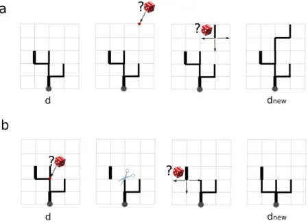
2.1.5. Neighbour state process: random pruning and branching
During simulated annealing, neighbouring random states for digraph d are generated (see line 7 in algorithm 1). A neighbour state is based on
random pruning (Fig. 1-b) and branching (Fig. 1-a) of the d graph as depicted on figure1 on a virtual example.
Figure 1: A neighbour state of tree d generated through random branching (a) or random pruning (b) processes. The two wide black segments are fixed parts of the network and the wide grey point corresponds to the tree root (outlet).
In this process, an edge belonging to the (ul− uf2) set is first randomly
selected (selection among the uncertain reaches), and two cases are therefore distinguished:
• If this selected edge already belongs to the ud digraph set of edges,
then the directed sub-graph (branch) upstream of the ending vertex of this edge is first pruned from digraph d to form dnew. Second, a
re-branching process is selected through a binary process with a prob-ability of 0.5. If selected, this re-branching process connects each of
the uf edges belonging to the upstream sub-graph with same
sequen-tial branching process as was used for the inisequen-tialisation of d0, and this
new branch is added to dnew.
• If the selected edge does not belong to (ud), a random walk
start-ing from its end node, reachstart-ing one of the d vertices, is performed. Consequently, a new branch is added to form dnew.
Due to its construction, this neighbour process allows the exploration of the entire l lattice for the reconstruction of d.
2.1.6. Energy functions
The choice of the energy function in the algorithm1governs the objective properties for the reconstructed networks. Here, we chose a bi-objective energy function. Our aim was that a reconstructed network should:
• converge to a target overall cumulative network length related to the extent of the catchment: this defines the catchment objective catch ; by using this convergence criterion, it is assumed that in future cases, the drainage network density or the cumulative length of a catchment can be predicted from environmental or anthropogenic variables (e.g., soil, catchment morphology and cultivated plot areas. . . ).
• reconnect a maximum number of fixed edges at the extent of the catch-ment: this defines the reconnection ratio objective ratio, equal to the fraction between the number of reconnected fixed edges and the num-ber of fixed edges;
The multi-objective energy function is energy = max(e1, e2), where
catchment energy: e1 = |Ld−catch|σ1 with σ1= catch ∗ γ1
reconnection ratio energy: e2 =
|Lf ∈d−Lf|
σ2 with σ2= Lf ∗ γ2
In these formulations, Ld=Pv∈udlength(v), Lf =Pv∈uf length(v),
Lf ∈dPv∈(ud&uf)length(v) denotes the cumulative length of f , d and f ,
respectively, within d edges. γ1, γ2 are convergence tuning parameters that
permit the differential adjustment of each of the objectives (e1, e2) relative
to the unique emax parameter.
Due to the construction of these formulations, all of the energies have normalised magnitude ranging from 0 to 1.
2.1.7. Simulated annealing decreasing temperature law
The simulated annealing initial decreasing temperature law follows the commonly employed equation:
Tk= Tini∗ (αk) (2)
where:
• δ = max(1,(Ll−catch)
catch ∗ 0.5)
• Tini = 0.51δ
The initial temperature parameter δ was fixed to a ’great’ cost, divided by 2 and normalised by the target catchment cumulative length. The α parameter was fixed such that exp ( −0.2
(α( kmax 5 ))∗5
) approximates 0.1. Both 0.51 and 0.1 values were fixed arbitrarily after trials and errors tests since automated fitted parameters for simulated annealing is still an open question (Wright,2010). There were also fixed according to suggestions from Aarts et al. (2003) for initial temperature related to the maximal cost between
two neighbouring solutions and from Zhang et al. (2010) in order to get a rejection rate of about 5-10 %.
2.2. Evaluating the ADN simulations with drainage network similarity met-rics
The previous subsection showed the way an ADN would be reconstructed given the following information: r, the known outlet of the network; l, the plot boundary lattice graph valued by elevation, and f , the set of fixed network reaches used to condition the reconstruction.
To assess the accuracy of the proposed ADN mapping method with re-spect to the f data or algorithm parameters, we computed the ditree network similarities based on scalar metrics. Theses metrics were used to compare each of the simulated ADNs to the actual one and, consequently, the forest dissimilarity distribution was computed.
As the objective function in algorithm 1 already uses global network geometry criteria (the drainage density), we chose to develop two comple-mentary network similarity metrics based on: 1) network topography and 2) network topology.
2.2.1. ADN topographical similarity metric
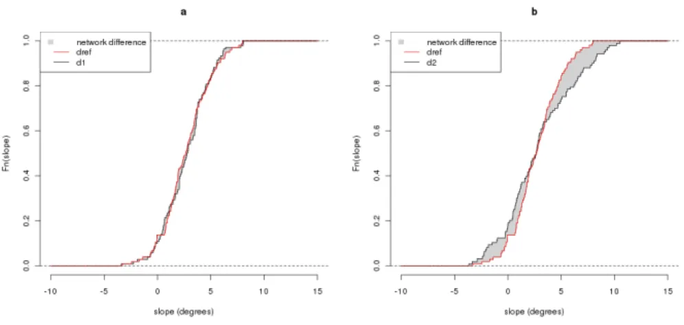
The topography of an ADN is fully contained in the slope of its network reaches. To summarize these slope distributions, any single synthetic slope statistic (e.g., mean and quantile) performs poorly. Therefore, we chose to use a metric based on the cumulative distribution of edge slopes. For a given network, we calculated the curve representing the cumulative distribution of slopes as follows: 1- for a given slope value θ, the proportion of the network length having slope smaller or equal than θ was computed; 2- this
was repeated for discretized and crescent values of the slope ranging from −90 to 90 degrees (see Figure2).
For two networks, the topographical similarity corresponds to the area between the two curves. This metric ht can be defined as:
ht(d1, dref) = | Z 90 −90 Fi(θ)dθ − Z 90 −90 Fref(θ)dθ|, (3)
where θ denotes the slope in degrees and Fi(θ) denotes the empirical
cumulative distribution function of the network slopes in relative cumulative lengths.
Figure 2: ADN topographical similarity computation through empirical cumulative edge slope distribution difference (grey areas): example of small (a) and great (b) dissimilarities for ditree d1 and d2 compared to dref
2.2.2. ADN topological similarity metric
Methods for the computation of the similarity between tree topologies have previously been developed in computational science to answer
prob-lems related to character chains, phylogenetic tree comparisons or the de-scription of deciduous tree architecture (Ferraro and Godin, 2000). These methods are all based on the Robinson-Foulds metric (Day, 1985) or Lev-enshtein or Jaro-Winkler distances (Jaro, 1985). These metrics are dedi-cated to valued trees with qualitative node labels. However, this is clearly not the problem in our case. In hydrology, topological characterisation of drainage networks is usually based on the Horton-Strahler, Shreve or Toku-naga upstream-downstream edge or node taxonomies (Barker et al.,1973). However, for a given ditree, these taxonomies cannot be easily reduced to a single value: it is usually represented in vectors or matrices as a branching matrix based on bi-order distributions, i.e. distributions of the twostrahler orders for stream joining downstream (Janey,1992, chapitre3).
To address this problem, we chose to develop the simple similarity met-ric hc, as proposed initially by Moslonka-Lefebvre et al. (2010) for
com-parison of gully networks in badlands extracted from remote sensing data (Thommeret et al.,2010). This metric is the distance between the Strahler barycenters of networks, where the Strahler barycenter of a network is the weighted barycenter of the network edge upstream nodes, with weights equal to Strahler orders: hc(d1, d2) = distance(G1, G2) (4) • xG1 = 1 P iw1i P iw1ix1i ; yG1 = 1 P iw1i P
iw1iy1i are the coordinates
of the d1 Strahler barycenter tree;
• xG2 = P1 jw2j P jw2jx2j ; yG2 = 1 P jw2j P
jw2jy2j are the coordinates
• w1i, w2j denotes the Strahler order of a node equal to that of the edge
for which the node is the upstream for trees d1, d2respectively. x1i, x2j
and y1i, y2j denote the coordinates of the edge upstream vertices of
trees d1, d2 respectively.
This unique metric combines the topology, geometry and geography of the network. It is further simply considered as the topological similarity metric.
3. Case study
3.1. The Muscat catchment and drainage network 3.1.1. Study site
The study area used here is the 2.6-km2 Muscat catchment located in the Languedoc region (south of France). This area was selected as being representative of the Languedocian vineyard landscape, where linear ele-ments play a major role in hydrological transfers. The area is successively composed of plateaus, sloping areas with terraces, gentle foot slopes formed from alluvial and colluvial deposits and a flat depression from upstream to downstream. The study area includes the Roujan elementary catchment, which has been equipped for conducting measurements of pollution, erosion and flooding since 1992 (Voltz and Albergel,2002). The drainage network drains cultivated plots and prevents erosion in the case of major runoff events. The positioning of the reaches that comprise most of this network within the landscape is highly variable and is highly dependent on reach functions. When the reach function is to capture surface waters, as in the case of high slopes, they are perpendicular to the terrain slope, especially
at the footstep of terrassettes. When the reach function is water trans-port, the reaches follow the slope direction. When reach function is to drain subsurface waters, there is no evident relationship with the local relief. 3.1.2. The actual Muscat drainage network
The actual drainage network of the studied catchment was exhaustively surveyed in 2004. It contains 239 edges and 240 nodes with 123 sources and 116 confluences (Fig. 3-a). Its cumulative length is 23,995 m that defines the catch parameter value.
Figure 3: The Muscat catchment data: a) the cultural plot lattice depicted on the 5-m hillshaded DTM; b) the actual drainage network in blue, with the reach width related to Strahler order ranging from 1 to 5; c) the plot lattice with the set f of known edges (blue:
c
BD-Topo for f2, red: remote sensing for f1)
3.1.3. The plot lattice and DTM data
For this catchment, a cultivated connected plot lattice containing 2,645 edges and 1,079 nodes was used (Fig. 3-b). The elevation was assigned to
each vertex of this lattice based on a 5-m resolution DTM having a random error of σz= 1m for the standard deviation. There is no internal sink within
this lattice that can trap random directed walks. 3.1.4. The ADN conditioning data
We used the whole set of known edges, f , to condition the reconstruction, as depicted in Figure3-c. This set was produced from:
• remote sensing detection based on LIDAR raw data (red lines). Re-mote sensing provides disconnected reaches, which may represent false detection, with a probability of 0.17 of false detection for upstream reaches that were not previously mapped in a geographical database. The cumulative length of the reaches is 15,400 m, i.e., 47% of the ac-tual network cumulative length. This set of fixed reaches corresponds to the f1 edge set because the direction of the reaches is unknown.
• the c BD-Topo-geographical database for hydrographic networks for the main downstream reaches (blue). Their cumulative length is 2,500 m, i.e., 7.5% of the actual network. This set of fixed reaches corre-sponds to the f2 edge set, which has a known direction.
• r which is the known outlet of the network that we want to reconstruct. Although it is not appropriate (no edge), we further consider that r can be the extreme case for the f conditioning data: only the outlet is fixed.
4. Results: reconstructed ADN on the Muscat catchment 4.1. Convergence efficiency
Beginning from the cultivated plot lattice shapefiles, algorithms were developed in the R statistical computing program (Ihaka and Gentleman,
1996) using the shapefiles and e1076 libraries (Team,2009). It took 9, 7.2 and 48 minutes on average to reconstruct a network using the (f = r), (f = f2) (f = f1 + f2) sets for conditioning, respectively, on a dual core
PC with 1 GB RAM. Additionally, r, f2, f1+ f2 denote the three exclusive
cases of f fixed edges used to condition the reconstruction.
The emax, γ1, γ2, kmaxparameters were adapted depending on the f
con-ditioning data:
• when using r or f2 to condition the reconstruction, the convergence
parameters were γ1= 1, γ2 = 1, emax= 0.01 and kmax = 500.
• when using f1+ f2 to condition the reconstruction, it took a long time
to achieve convergence due to both considerable constraints related to lattice space exploration and a multi-objective (e1, e2) dilemma (Kung
et al., 1975). A Pareto optimum providing a compromise between the duration of and the objective of accuracy for the simulation was found with the following convergence parameters: γ1 = 1, γ2 = 4 for
emax = 0.05 and kmax= 2, 000.
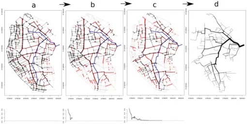
In Figure4, the evolution of energy within the simulated annealing pro-cess using f = (f1+ f2), as well as according to the reconstructed digraph,
Figure 4: Simulated annealing algorithm1 intermediary states: a) initial digraph and energy for k = 0; b) digraph and energy at iteration k = 30; c) digraph and energy at final iteration k = 309; d) final obtained ditree. On the top, the lattice edges are depicted in grey; the directed reconstructed graphs are indicated by black arrows. The fixed edges of f with a known direction ( c BD-Topo) are depicted in blue, and the fixed edges of f with an unknown direction (remote sensing) are depicted in red. On the bottom, the energy e is depicted as a function of k.
In Figure4, the cumulative length of the initial digraph d passing through at least 95 % of the f edges covers most of the lattice l and, consequently, has a high energy e due to its overly long cumulative network length. At the intermediary state (k = 30), the energy is still high (around 0.2) due to a weak f edge reconnection, and the graph d is segmented in spatial clusters due to a great amount of pruning occurring when the temperature remains high enough. For larger iterations (k > 200), the energy slowly decreases with local pruning and branching to converge to the desired maximum level of energy (emax= 0.05) at iteration k = 308.
4.1.1. Reconstructed network variability
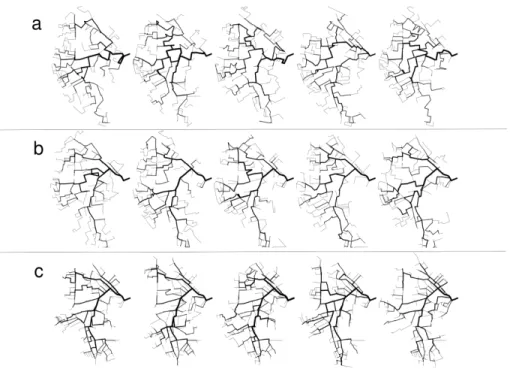
Three forests of 100 reconstructed networks were built using r, f2, f1+ f2
to condition the reconstruction. Some of the networks sampled from these three forests are depicted in Figure5.
Figure 5: Example of five reconstructed networks using a) r, b) f2, c) f1+f2. All networks
are depicted with a line width related to their Strahler orders.
In this Figure, the reconstructed networks look realistic compared to the actual network (Figure 3-b). However, differences appear between cases r, f2 and f1+ f2. The topology seems less realistic for r than for f1 + f2.
However, the reconstructed networks look more realistic in the parts of the catchment where the actual main branches belong to the f2 edges.
4.2. Conditioning data effects on network similarities
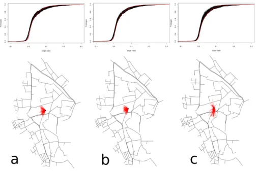
Similarities of the reconstructed network forests using the different sets of fixed edges r, f2 and f1+ f2 were computed. The ht, hcsimilarity
distri-butions can be deduced from the graphs in Figure6.
Figure 6: Similarity distribution of forests using a) r, b) f2, c) f1+ f2. On the top, the
Fθ(slope) curves are depicted for the actual network (red) and the reconstructed networks
(black). On the bottom, the Strahler barycenter of the actual network is depicted by the black point from which red segments join the reconstructed network Strahler barycenters.
The top part of Figure 6 shows that the ht topographic similarity
dis-tribution is quite similar for r and f2. For f1+ f2, the slope distribution
appears to be of higher magnitude where the slope is greater than 0.2 rad. In all cases, the reconstructed network slopes are not totally centred on the
actual slope distribution and overestimate very low and negative slopes. The bottom part of Figure 6 shows that the hc topological similarity
distribu-tion is once again quite similar for r and f2, but with a lower magnitude for
f2. For f1+ f2, the topological dissimilarities appear to be better centred,
despite an apparently higher magnitude.
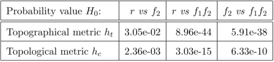
Mean and standard deviation statistics were computed from these dif-ferent similarity distributions (Table 4.2) and then tested for statistically significant differences, using a two sample comparison Welch T test (Ta-ble 4.2). These statistics confirm that the use of f2 slightly improves the
topological and topographical similarities of the networks.
f : r f2 f1+ f2
Actual edges length (%) 42.6 45.6 57.5
¯ Ld 23850.5 23868.5 24763 ¯ ht 0.00101 0.00118 0.00394 σht 0.00201 0.00217 0.00275 ¯ hc 244.9 230.2 197.5 σhc 23.5 22.2 37.5
Table 1: Dissimilarities statistics
Despite having a higher ratio of fixed reaches compared to f2, the use of
f1+ f2 significantly improves the topological similarity of the networks but
Probability value H0: r vs f2 r vs f1f2 f2 vs f1f2
Topographical metric ht 3.05e-02 8.96e-44 5.91e-38
Topological metric hc 2.36e-03 3.03e-15 6.33e-10
Table 2: Welch two sample T test probability values
This is probably due to the locations of the f1 edges corresponding to
false remote sensing detection (Bailly et al.,2008), with more being located in the terraced hillslides of the Muscat catchment and favouring higher slopes in the networks. This could also be produced from the necessary emax
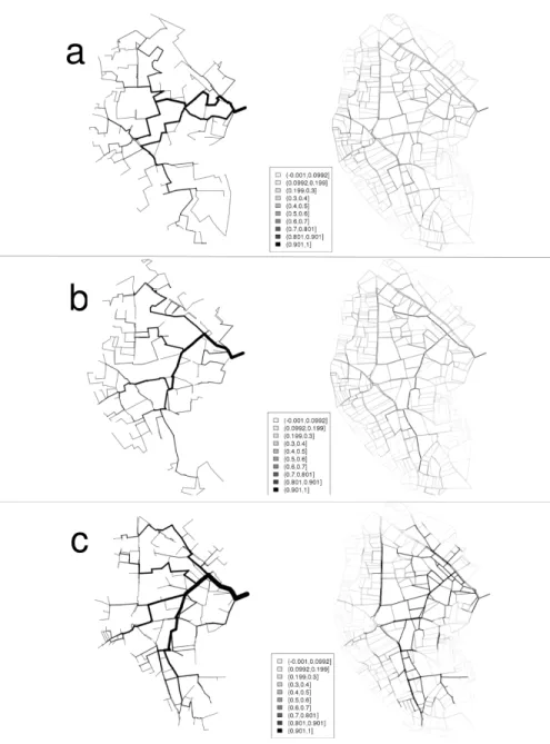
dif-ference (relaxation), favouring added edges upstream on terraced hillslides. From the reconstructed forests and similarity distributions, a median network corresponding the reconstructed network with minimized median orders on similarity metrics was computed. This median network is showed using a) r, b) f2, c) f1 + f2 on the left of figure 7. In addition,
uncer-tainties in network reconstruction was computed through the frequency in reconstructed networks for each one of the cultivated plot boundaries lattice edge. These uncertainties are also mapped using a) r, b) f2, c) f1+ f2 on
the right on figure7. On this figure, the median tree using f1+ f2 looks the
more realistic and close to the actual one. As expected, uncertainties are higher on upstream areas corresponding to terraced hillslides.
5. Conclusions
In this study, a simulated spatial annealing algorithm for the stochastic reconstruction of artificial drainage networks was proposed. This algorithm uses the plot boundary lattice of a cultivated landscape directed by DTM
Figure 7: The median reconstructed network (left) and frequencies of lattice edges in reconstructed networks (right) using a) r, b) f2, c) f1+ f2.
elevation and is conditioned by unconnected known reaches. A number of equi-probable drainage networks connected to a given outlet with an
upstream-downstream ditree structure were produced. They follow a given cumulative length and maximise the reconnection of unconnected known reaches. Randomness in the algorithm comes from upstream-downstream random walks along the cultivated plot lattice and according to random pruning or branching processes in the network.
This algorithm can be used to complete or interpolate from known re-gions of networks produced from ground observations, geographical databases or remote sensing detection. It also permits the representation of uncer-tainties in drainage network mapping through multiple realisations of the algorithm.
The results of applying the algorithm to the Muscat catchment with or without using edges detected from airborne scanner laser, from the c BD-Topo database, showed quite realistic reconstructed networks in all cases; the simulations are highly constrained by the 3D structure of the plot lat-tice. However, a quantitative study of the geometric, topographical and topological properties of the reconstructed networks using different crite-ria than were used as the objectives for simulated annealing resulted in equivocal conclusions. Adding uncertain information from remote sensing of network locations does not always benefit the model, as it increases the biases of some parameters of the network and reduces others, while adding considerable constraints related to convergence and a long duration to the reconstruction process. It appears that the location, rather than the ratio, of the unconnected true reaches is more important. This assumption could be assessed in future studies using the proposed reconstruction algorithm.
Another question regarding the realistic character of the simulations obtained using this algorithm is related to the final usage of the mapped drainage networks. In this case, only descriptive criteria were used, but
cri-teria based on the hydrological functioning of the simulated networks also need to be assessed. In other words, do uncertainties in drainage network maps resulting from the available data and the proposed algorithm have a significant influence when they are propagated into a given hydrological model ?
The proposed algorithm is generic and can be extended to other works, to other catchments and even using objectives related to other net-work properties. Its main requirements are a cultivated plot lattice that can be valued with elevations and known outlets. It also requires a value of the cumulative length of the network to be simulated. This drainage density is expected to be predicted spatially in future studies.
Acknowledgement(s)
The authors are grateful to the INSU-ECCO-PNRH French national pro-gram in hydrology for its general support of this study, which is included
in the MOBHYDIC project. They are also grateful to the
Languedoc-Roussillon region for the funding of this study through a Ph.D program.
Aarts, E., Korst, J., vanLaarhoven, P., 2003. Local search in combinato-rial optimization. Princeton: Princeton University Press, Ch. Simulated Annealing.
Amini, J., Blais, M. S. J., Lucas, C., Azizi, A., 2002. Automatic road-side extraction from large scale imagemaps. International Journal of Applied Earth Observation and Geoinformation 4, 95–107.
Bailly, J.-S., Lagacherie, P., Millier, C., Puech, C., Kosuth, P., 2008. Agrar-ian landscapes linear features detection from lidar: application to artifi-cial drainage networks. International Journal of Remote Sensing 29(12), 3489–3508.
Baltsavias, E., Zhang, C., 2005. Automated updating of road databases from aerial images. International Journal of Applied Earth Observation and Geoinformation 6, 199–213.
Barker, S. B., Cumminc, G., Horsfield, K., 1973. Quantitative morphometry of the branching structure of trees. J. theor. Biol. 40, 33–43.
Beven, K., Binley, A., 1992. The future of distributed models: Model cali-bration and uncertainty prediction. Hydrological processes 6, 279–298. Beven, K., Freer, J., 2001. Equifinality, data assimilation, and uncertainty
estimation in mechanistic modelling of complex environmental systems using the glue methodology. Journal of Hydrology 249 (1-4), 11–29. Bouldin, J., Farris, J., Moore, M., Cooper, C., 2004. Vegetative and
struc-tural characteristics of agriculstruc-tural drainages in the mississippi delta land-scapes. Environmental Pollution 132 (3), 403–411.
Carpentier, A., Paillisson, J., Mariona, L., Feunteun, E., Baisez, A., Rigaud, C., 2003. Trends of a bitterling (rhodeus sericeus) population in a man-made ditch network. C. R. Biologies 326, 166–173.
Comoretto, L., 2003. Analyse des chemins de l’eau d’un petit bassin rural sur mnt thr. Master’s thesis, Universit de Montpellier II.
hotspots? the floral and butterfly diversity of green lanes. Biological Con-servation 121 (4), 579–584.
Dages, C., Voltz, M., Lacas, J., Huttel, O., Negro, S., Louchart, X., 2008. An experimental study of water table recharge by seepage losses from a ditch with intermittent flow. Hydrological Processes 22, 3555–3563. Day, W., 1985. Optimal algorithms for comparing trees with labeled leaves.
Journal of Classification 1 (1).
Descombes, X., van Lieshout, M., Stoica, R., Zerubia, J., August 2001. Parameter estimation by a markov chain monte carlo technique for the candy-model. In: IEEE Workshop on Statistical Signal Processing. papier invit, Singapour.
Duke, G., Kienzle, S., Johnson, D., Byrne, J., 2006. Incorporating ancillary data to refine anthropogenically modified overland flow paths. Hydrolog-ical Processes 20, 1827–1843.
Fairfield, J., Leymarie, P., 1991. Correction to ?drainage networks from grid digital elevation models? Water Resources Research 27 (10), 2809. Ferraro, P., Godin, C., 2000. A distance measure between plant
architec-tures. Ann. For. Sci. 57, 445?461.
Garcia, M., Camarasa, A., 1999. Use of geomorphological units to improve drainage network extraction from a dem : Comparison between automated extraction and photointerpretation methods in the carraixet catchment (valencia, spain). International Journal of Applied Earth Observation and Geoinformation 1 (3-4), 187–195.
Heipke, C., Mayer, H., Wiedemann, C., Jamet, O., 1997. Evaluation of automatic road extraction. International Archives of Photogrammetry and Remote Sensing 23, 151–160.
Ihaka, R., Gentleman, R., 1996. R: A language for data analysis and graph-ics. Journal of Computational and Graphical Statistics 5 (3), 299–314. Janey, N., 1992. Modelisation et synthese d’image d’arbres et de bassins
fluviaux associant methodes combinatoires et plongement automatique d’arbres et cartes planaires. Ph.D. thesis, Universite de Franche-Comte. Jaro, M., 1985. Advances in record linking methodology as applied to the
1985 census of tampa florida. Journal of the American Statistical Society 84 (406), 414–420.
Kruskal, J., 1956. On the shortest spanning subtree of a graph and the traveling salesman problem. Proceedings of the American Mathematical Society 6, 48–50.
Kung, H., Luccio, F., Preparata, F., 1975. On finding the maxima of a set of vectors. Journal of the ACM 22 (4), 469–476.
Lacoste, C., Descombes, X., Zerubia, J., 2005. Point processes for unsuper-vised line network extraction in remote sensing. IEEE Transactions on Pattern Analysis and Machine Intelligence 27 (10), 1568–1579.
Lagacherie, P., Diot, O., Domange, N., Gouy, V., Floure, C., Kao, C., Moussa, R., Robbez-Masson, J., Szleper, V., 2006. An indicator approach for describing the spatial variability of human-made stream network in regard with herbicide pollution in cultivated watersheds. Ecological indi-cators 6, 265–279.
Lagacherie, P., Rabotin, M., Colin, F., Moussa, R., Voltz, M., 2010. Geo-mhydas: A landscape discretization tool for distributed hydrological mod-eling of cultivated areas. Computers & Geosciences 36 (8), 1021–1032. Lantuejoul, C., 2002. Geostatistical Simulation: Models and Algorithms.
Springer Verlag.
Mariani, R., Deseilligny, M. P., Labiche, J., Lecourtier, Y., Mullot, R., 1995. Image Analysis Applications and Computer Graphics. Vol. 1024/1995. Springer Berlin, Ch. Geographic map understanding. Algorithms for hy-drographic network reconstruction, pp. 514–515.
Molly, I., Stepinski, T., 2007. Automatic mapping of valley networks on mars. Computers & Geosciences 33, 728–728.
Moslonka-Lefebvre, M., Kervinio, Y., Mejri, R., Pointud, L., 2010. Meth-odes de comparaison de formes arborescentes: application aux reseaux hydrographiques sur sig. Tech. rep., AgroParisTech-ENGREF.
Moussa, R., Voltz, M., Andrieux, P., 2002. Effects of the spatial organization of agricultural management on the hydrological behaviour of a farmed catchment during flood events. Hydrological Processes 16, 393–412. O’Callaghan, J., Mark, D., 1984. The extraction of drainage networks from
digital elevation data. Computer Vision, Graphics, and Image Processing 28 (3), 323–344.
Pita, R., Mira, A., Beja, P., 2006. Conserving the cabrera vole, micro-tus cabrerae, in intensively used mediterranean landscapes,. Agriculture, Ecosystems and Environment 115 (3), 1–5.
Prim, R., 1957. Shortest connection networks and some generalizations. Bell System Technical Journal 36, 1389–1401.
Soille, P., Gratin, C., 1994. An efficient algorithm for drainage network extraction on dems. Journal of Visual Communication and Image Repre-sentation 5, 181–189.
Spitzer, F., 1970. Principles of the Random Walk. Vol. 34 of Graduate Texts in Mathematics. Springer-Verlag.
Stoica, R., Descombes, X., Zerubia, J., 2004. A gibbs point process for road extraction in remotely sensed images. International Journal of Computer Vision 57 (2), 121–136.
Team, R. D. C., 2009. R: A Language and Environment for Statistical Com-puting. R Foundation for Statistical Computing, Vienna, Austria, ISBN 3-900051-07-0.
URLhttp://www.R-project.org
Thommeret, N., Bailly, J. S., Puech, C., 2010. Extraction of thalweg net-works from dtms: application to badlands. Hydrology and Earth Sciences System 14, 1527–1536.
VanGroenigen, J., Stein, A., 1998. Constrained optimization of spatial sam-pling using continuous simulated annealing. Journal of Environmental Quality 27, 1078–1086.
Varado, N., 2004. Contribution au d´eveloppement d’une mod´elisation hy-drologique distribu´ee. application au bassin versant de la donga au b´enin. Ph.D. thesis, Universit´e de Grenoble.
Vassilopoulos, A., Evelpidou, N., Bender, O., Krek, A., 2008. Geoinforma-tion Technologies for Geo-Cultural Landscapes: European Perspectives. CRC Press.
Voltz, M., Albergel, J., 2002. Omere: Observatoire mediterraneen de l’environnement rural et de l’eau: Impact des actions anthropiques sur les transferts de masse dans les hydrosystemes mediterraneens ruraux. propo-sition d’observatoire de recherche en environnement. Tech. rep., Ministere de la Recherche.
Wilson, J., Lam, C., Deng, Y., 2007. Comparison of the performance of flow-routing algorithms used in gis-based hydrologic analysis. Hydrologi-cal Processes 21, 1026–1044.
Wright, M., 2010. Automating parameter choice for simulated annealing. Tech. rep., Lancaster university.
Zhang, L., M’Hallah, R., Leung, S., 2010. A simulated annealing with a new neighorhood structure based algorithm for high school timetabling problems. European Journal of Operational Research 203 (3), 550–558.