HAL Id: hal-01095123
https://hal.inria.fr/hal-01095123
Submitted on 18 Dec 2014
HAL is a multi-disciplinary open access
archive for the deposit and dissemination of
sci-entific research documents, whether they are
pub-lished or not. The documents may come from
teaching and research institutions in France or
L’archive ouverte pluridisciplinaire HAL, est
destinée au dépôt et à la diffusion de documents
scientifiques de niveau recherche, publiés ou non,
émanant des établissements d’enseignement et de
recherche français ou étrangers, des laboratoires
Predicate-aware, makespan-preserving software
pipelining of scheduling tables
Thomas Carle, Dumitru Potop-Butucaru
To cite this version:
Thomas Carle, Dumitru Potop-Butucaru. Predicate-aware, makespan-preserving software pipelining
of scheduling tables. ACM Transactions on Architecture and Code Optimization, Association for
Computing Machinery, 2014, 11, pp.1 - 26. �10.1145/2579676�. �hal-01095123�
Predicate-aware, makespan-preserving
software pipelining of scheduling tables
1 Thomas Carle, INRIA Paris-RocquencourtDumitru Potop-Butucaru, INRIA Paris-Rocquencourt
We propose a software pipelining technique adapted to specific hard real-time scheduling problems. Our technique optimizes both computation throughput and execution cycle makespan, with makespan being prioritary. It also takes advantage of the predicated execution mechanisms of our embedded execution plat-form. To do so, it uses a reservation table formalism allowing the manipulation of the execution conditions of operations. Our reservation tables allow the double reservation of a resource at the same dates by two different operations, if the operations have exclusive execution conditions. Our analyses can determine when double reservation is possible even for operations belonging to different iterations.
1. INTRODUCTION
In this paper, we take inspiration from a classical compilation technique, namely software pipelining, in order to improve the system-level task scheduling of a specific class of embed-ded systems.
Software pipelining.Compilers are expected to improve code speed by taking advantage of micro-architectural instruction level parallelism [Hennessy and Patterson 2007].
Pipelin-ing compilers usually rely on reservation tables to represent an efficient (possibly optimal)
static allocation of the computing resources (execution units and/or registers) with a tim-ing precision equal to that of the hardware clock. Executable code is then generated that enforces this allocation, possibly with some timing flexibility. But on VLIW architectures, where each instruction word may start several operations, this flexibility is very limited, and generated code is virtually identical to the reservation table. The scheduling burden is mostly supported here by the compilers, which include software pipelining techniques [Rau and Glaeser 1981; Allan et al. 1995] designed to increase the throughput of loops by allowing one loop cycle to start before the completion of the previous one.
Static (offline) real-time scheduling. A very similar picture can be seen in the system-level design of safety-critical real-time embedded control systems with distributed (parallel,
multi-core) hardware platforms. The timing precision is here coarser, both for starting dates,
which are typically given by timers, and for durations, which are characterized with worst-case execution times (WCET). However, safety and efficiency arguments[Fohler et al. 2008] lead to the increasing use of tightly synchronized time-triggered architectures and execu-tion mechanisms, defined in well-established standards such as TTA, FlexRay[Rushby 2001], ARINC653[ARINC653], or AUTOSAR[AUTOSAR]. Systems based on these platforms typ-ically have hard real-time constraints, and their correct functioning must be guaranteed by a schedulability analysis. In this paper, we are interested in statically scheduled systems where resource allocation can be described under the form of a reservation/scheduling table which constitutes, by itself, a proof of schedulability. Such systems include:
— Periodic time-triggered systems [Caspi et al. 2003; Zheng et al. 2005; Monot et al. 2010; Eles et al. 2000; Potop-Butucaru et al. 2010] that are naturally mapped over ARINC653, AUTOSAR, TTA, or FlexRay.
— Systems where the scheduling table describes the reaction to some sporadic input event (meaning that the table must fit inside the period of the sporadic event). Such systems
1
This work was partially funded by the FUI PARSEC project. Preliminary results of this work are also available online as the Chalmers’ master thesis of the first author http://publications.lib.chalmers.se/ records/fulltext/146444.pdf.
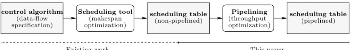
This paper scheduling table (non-pipelined) Pipelining (throughput optimization) scheduling table (pipelined) (data-flow specification) (makespan Scheduling tool optimization) control algorithm Existing work
Fig. 1. Proposed pipelined scheduling flow
can be specified in AUTOSAR, allowing, for instance, the modeling of computations syn-chronized with engine rotation events [Andr´e et al. 2007].
— Some systems with a mixed event-driven/time-driven execution model, such as those syn-thesized by SynDEx[Grandpierre and Sorel 2003].
Synthesis of such systems starts from specifications written in domain-specific formalisms such as Simulink or SCADE[Caspi et al. 2003]. These formalisms allow the description of concurrent data computations and communications that are conditionally activated at each cycle of the embedded control algorithm depending on the current input and state of the system.
The problem. The optimal scheduling of such specifications onto platforms with multiple, heterogenous execution and communication resources (distributed, parallel, multi-core) is NP-hard regardless of the optimality criterion (throughput, makespan, etc.) [Garey and Johnson 1979]. Existing scheduling techniques and tools [Caspi et al. 2003; Zheng et al. 2005; Grandpierre and Sorel 2003; Potop-Butucaru et al. 2010; Eles et al. 2000] heuristically solve the simpler problem of synthesizing a scheduling table of minimal length which implements one generic cycle of the embedded control algorithm. In a hard real-time context, minimizing table length (i.e. the makespan, as defined in the glossary of Fig. 2) is often a good idea, because in many applications it bounds the response time after a stimulus.
But optimizing makespan alone relies on an execution model where execution cycles can-not overlap in time (no pipelining is possible), even if resource availability allows it. At the same time, most real-time applications have both makespan and throughput requirements, and in some cases achieving the required throughput is only possible if a new execution cycle is started before the previous one has completed.
This is the case in the electronic control units (ECU) of combustion engines. Starting from the acquisition of data for a cylinder in one engine cycle, an ECU must compute the ignition parameters before the ignition point of the same cylinder in the next engine cycle (a makespan constraint). It must also initiate one such computation for each cylinder in each engine cycle (a throughput constraint). On modern multiprocessor ECUs, meeting both constraints requires the use of pipelining[Andr´e et al. 2007]. Another example is that of systems where a faster rate of sensor data acquisition results in better precision and improved control, but optimizing this rate must not lead to the non-respect of requirements on the latency between sensor acquisition and actuation. To allow the scheduling of such
systems we consider here the static scheduling problem of optimizing both makespan and throughput, with makespan being prioritary.
Contribution. To (heuristically) solve this optimization problem, we use a two-phase scheduling flow that can be seen as a form of decomposed software pipelining [Wang and Eisenbeis 1993; Gasperoni and Schwiegelshohn 1994; Calland et al. 1998]. As pictured in Fig. 1, the first phase of this flow consists in applying one of the previously-mentioned makespan-optimizing tools. The result is a scheduling table describing the execution of one generic execution cycle of the embedded control algorithm with no pipelining.
The second phase uses a novel software pipelining algorithm, introduced in this paper, to significantly improve the throughput without changing the makespan and while
preserv-Concept Description
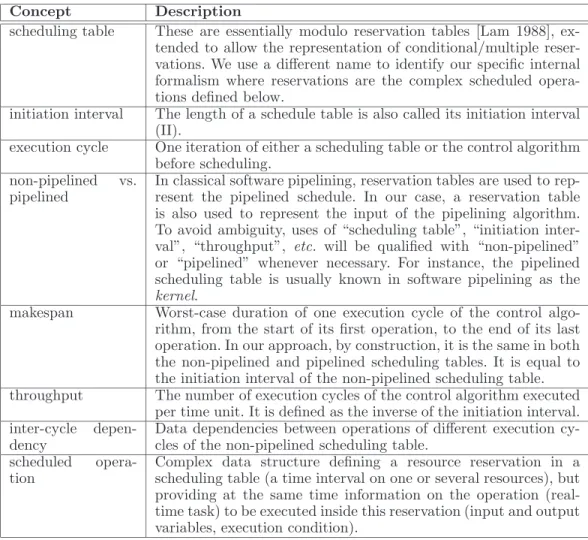
scheduling table These are essentially modulo reservation tables [Lam 1988], ex-tended to allow the representation of conditional/multiple reser-vations. We use a different name to identify our specific internal formalism where reservations are the complex scheduled opera-tions defined below.
initiation interval The length of a schedule table is also called its initiation interval (II).
execution cycle One iteration of either a scheduling table or the control algorithm before scheduling.
non-pipelined vs. pipelined
In classical software pipelining, reservation tables are used to rep-resent the pipelined schedule. In our case, a reservation table is also used to represent the input of the pipelining algorithm. To avoid ambiguity, uses of “scheduling table”, “initiation inter-val”, “throughput”, etc. will be qualified with “non-pipelined” or “pipelined” whenever necessary. For instance, the pipelined scheduling table is usually known in software pipelining as the
kernel.
makespan Worst-case duration of one execution cycle of the control algo-rithm, from the start of its first operation, to the end of its last operation. In our approach, by construction, it is the same in both the non-pipelined and pipelined scheduling tables. It is equal to the initiation interval of the non-pipelined scheduling table. throughput The number of execution cycles of the control algorithm executed
per time unit. It is defined as the inverse of the initiation interval. inter-cycle
depen-dency
Data dependencies between operations of different execution cy-cles of the non-pipelined scheduling table.
scheduled opera-tion
Complex data structure defining a resource reservation in a scheduling table (a time interval on one or several resources), but providing at the same time information on the operation (real-time task) to be executed inside this reservation (input and output variables, execution condition).
Fig. 2. Glossary of terms used in this paper. All notions are formally defined later
ing the periodic nature of the system. The approach has the advantage of simplicity and generality, allowing the use of existing makespan-optimizing tools.
The proposed software pipelining algorithm is a very specific and constrained form of
mod-ulo scheduling [Rau 1996]. Like all modmod-ulo scheduling algorithms, it determines a shorter initiation interval for the execution cycles (iterations) of the control algorithm, subject to
resource and inter-cycle data dependency constraints. Unlike previous modulo scheduling algorithms, however, it starts from an already scheduled code (the non-pipelined scheduling table), and preserves all the intra-cycle scheduling decisions made at phase 1, in order to preserve the makespan unchanged. In other words, our algorithm computes the best
initi-ation interval for the non-pipelined scheduling table and re-organizes resource reserviniti-ations
into a pipelined scheduling table, whose length is equal to the new initiation interval, and which accounts for the changes in memory allocation.
We have implemented our algorithm into a pipelining tool that is used, as we desired, in conjunction with an existing makespan-optimizing scheduling tool. The resulting two-phase flow gives good results on architectures without temporal partitioning [ARINC653], like the previously-mentioned AUTOSAR or SynDEx-generated applications and, to a certain extent, applications using the FlexRay dynamic segment.
For applications mapped onto partitioned architectures (ARINC 653, TTA, or FlexRay, the static segment) or where the non-functional specification includes multiple release date, end-to-end latency, or periodicity constraints, separating the implementation process in two phases (scheduling followed by pipelining) is not a good idea. We therefore developed a single-phase pipelined scheduling technique documented elsewhere [Carle et al. 2012], but which uses (with good results) the same internal representation based on scheduling tables to allow a simple mapping of applications with execution modes onto heterogenous architectures with multiple processors and buses.
Outline
The remainder of the paper is structured as follows. Section 2 reviews related work. Section 3 formally defines scheduling tables. Sections 4 and 5 present the pipelining technique and provide and provide a complex example. Section 5 deals with data dependency analysis. Section 6 gives experimental results, and Section 7 concludes.
2. RELATED WORK AND ORIGINALITY
This section reviews related work and details the originality points of our paper. Perform-ing this comparison required us to relate concepts and techniques belongPerform-ing to two fields: software pipelining and real-time scheduling. To avoid ambiguities when the same notion has different names depending on the field, we define in Fig. 2 a glossary of terms that will be used throughout the paper.
2.1. Decomposed software pipelining.
Closest to our work are previous results on decomposed software pipelining [Wang and Eisen-beis 1993; Gasperoni and Schwiegelshohn 1994; Calland et al. 1998]. In these papers, the software pipelining of a sequential loop is realized using two-phase heuristic approaches with good practical results. Two main approaches are proposed in these papers.
In the first approach, used in all 3 cited papers, the first phase consists in solving the loop scheduling problem while ignoring resource constraints. As noted in [Calland et al. 1998], existing decomposed software pipelining approaches solve this loop scheduling problem by using retiming algorithms. Retiming [Leiserson and Saxe 1991] can therefore be seen as a very specialized form of pipelining targeted at cyclic (synchronous) systems where each operation has its own execution unit. Retiming has significant restrictions when compared with full-fledged software pipelining:
— It is oblivious of resource allocation. As a side-effect, it cannot take into account execution conditions to improve allocation, being defined in a purely data-flow context.
— It requires that the execution cycles of the system do not overlap in time, so that one operation must be completely executed inside the cycle where it was started.
Retiming can only change the execution order of the operations inside an execution cycle. A typical retiming transformation is to move one operation from the end to the beginning of the execution cycle in order to shorten the duration (critical path) of the execution cycle, and thus improve system throughput. The transformation cannot decrease the makespan but may increase it.
Once retiming is done, the second transformation phase takes into account resource con-straints. To do so, it considers the acyclic code of one generic execution cycle (after re-timing). A list scheduling technique ignoring inter-cycle dependences is used to map this acyclic code (which is actually represented with a directed acyclic graph, or DAG) over the available resources.
The second technique for decomposed software pipelining, presented in [Wang and Eisen-beis 1993], basically switches the two phases presented above. Resource constraints are considered here in the first phase, through the same technique used above: list scheduling of
DAGs. The DAG used as input is obtained from the cyclic loop specification by preserving only some of the data dependences. This scheduling phase decides the resource allocation and the operation order inside an execution cycle. The second phase takes into account the data dependences that were discarded in the first phase. It basically determines the fastest way a specification-level execution cycle can be executed by several successive pipelined ex-ecution cycles without changing the operation scheduling determined in phase 1 (preserving the throughput unchanged). Minimizing the makespan is important here because it results in a minimization of the memory/register use.
2.2. Originality.
In this paper, we propose a third decomposed software pipelining technique with two sig-nificant originality points, detailed below.
2.2.1. Optimization of both makespan and throughput.Existing software pipelining techniques are tailored for optimizing only one real-time performance metric: the processing throughput of loops [Yun et al. 2003] (sometimes besides other criteria such as register usage [Govindara-jan et al. 1994; Zalamea et al. 2004; Huff 1993] or code size [Zhuge et al. 2002]). In addition to throughput, we also seek to optimize makespan, with makespan being prioritary. Recall that throughput and latency (makespan) are antagonistic optimization objectives during scheduling [Benoˆıt et al. 2007], meaning that resulting schedules can be quite different (an example will be provided in Section 4.1.2).
To optimize makespan we employ in the first phase of our approach existing schedul-ing techniques that were specifically designed for this purpose [Caspi et al. 2003; Zheng et al. 2005; Grandpierre and Sorel 2003; Potop-Butucaru et al. 2010; Eles et al. 2000]. But the main contribution of this paper concerns the second phase of our flow, which takes the scheduling table computed in phase 1 and optimizes its throughput while keeping its makespan unchanged. This is done using a new algorithm that conserves all the allocation and intra-cycle scheduling choices made in phase 1 (thus conserving makespan guarantees), but allowing the optimization of the throughput by increasing (if possible) the frequency with which execution cycles are started.
Like retiming, this transformation is a very restricted form of modulo scheduling software pipelining. In our case, it can only change the initiation interval (changes in memory alloca-tion and in the scheduling table are only consequences). By comparison, classical software pipelining algorithms, such as the iterative modulo scheduling of [Rau 1996], perform a full mapping of the code involving both execution unit allocation and scheduling. Our choice of transformation is motivated by three factors:
— It preserves makespan guarantees.
— It gives good practical results for throughput optimization. — It has low complexity.
It is important to note that our transformation is not a form of retiming. Indeed, it allows for a given operation to span over several cycles of the pipelined implementation, and it can take advantage of conditional execution to improve pipelining, whereas retiming techniques work in a pure data-flow context, without predication (an example will be provided in Section 4.1.2).
2.2.2. Predication.For an efficient mapping of our conditional specifications, it is important to allow an independent, predicated (conditional) control of the various computing resources. However, most existing techniques for software pipelining [Allan et al. 1995; Warter et al. 1993; Yun et al. 2003] use hardware models that significantly constrain or simply prohibit predicated resource control. This is due to limitations in the target hardware itself. One common problem is that two different operations cannot be scheduled at the same date on a given resource (functional unit), even if they have exclusive predicates (like the branches
of a test). The only exception we know to this rule is predicate-aware scheduling (PAS) [Smelyanskyi et al. 2003].
By comparison, the computing resources of our target architectures are not a mere func-tional units of a CPU (as in classical predicated pipelining), but full-fledged processors such as PowerPC, ARM, etc. The operations executed by these computing resources are large sequential functions, and not simple CPU instructions. Thus, each computing resource al-lows unrestricted predication control by means of conditional instructions, and the timing overhead of predicated control is negligible with respect to the duration of the operations. This means that our architectures satisfy the PAS requirements. The drawback of PAS is that sharing the same resource at the same date is only possible for operations of the same cycle, due to limitations in the dependency analysis phase. Our technique removes this limitation (an example will be provided in Section 4.1.3).
To exploit the full predicated control of our platform we rely on a new intermediate representation, namely predicated and pipelined scheduling tables. By comparison to the modulo reservation tables of [Lam 1988; Rau 1996], our scheduling tables allow the explicit representation of the execution conditions (predicates) of the operations. In turn, this allows the double reservation of a given resource by two operations with exclusive predicates. 2.3. Other aspects
A significant amount of work exists on applying software pipelining or retiming techniques for the efficient scheduling of tasks onto coarser-grain architectures, such as multi-processors [Kim et al. 2012; Yang and Ha 2009; Chatha and Vemuri 2002; Chiu et al. 2011; Caspi et al. 2003; Morel 2005]. To our best knowledge, these results share the two fundamental limi-tations of other software pipelining algorithms: Optimizing for only one real-time metric (throughput) and not fully taking advantage of conditional execution to allow double allo-cation of resources.
Minor originality points of our technique, concerning code generation and dependency analysis will be discussed and compared with previous work in Sections 4.4 and 5.
3. SCHEDULING TABLES
This section defines the formalism used to represent the non-pipelined static schedules produced by phase 1 of our scheduling flow and taken as input by phase 2. Inspired from [Potop-Butucaru et al. 2010; Grandpierre and Sorel 2003], our scheduling table formalism remains at a significantly lower abstraction level. The models of [Potop-Butucaru et al. 2010; Grandpierre and Sorel 2003] are fully synchronous: Each variable has at most one value at each execution cycle, and moving one value from a cycle to the next can only be done through explicit delay constructs. In our model, each variable (called a memory cell) can be assigned several times during a cycle, and values are by default passed from one execution cycle to the next.
The lower abstraction level means that time-triggered executable code generated by any of the previously-mentioned scheduling tools can directly be used as input for the pipelining phase. Integration between the scheduling tools and the pipelining algorithm defined next is thus facilitated. The downside is that the pipelining technique is more complex, as detailed in Section 4.4.2.
3.1. Architecture model
We model our multi-processor (distributed, parallel) execution architectures using a very simple language defining sequential execution resources, memory blocks, and their
intercon-nections. Formally, an architecture model is a bipartite undirected graph A =< P, M, C >,
with C ⊆ P × M. The elements of P are called processors, but they model all the computa-tion and communicacomputa-tion devices capable of independent execucomputa-tion (CPU cores, accelerators, DMA and bus controllers, etc.). We assume that each processor can execute only one
oper-v2
v1
P1 M1 P2 M2 P3
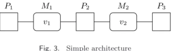
Fig. 3. Simple architecture
ation at a time. We also assume that each processor has its own sequential or time-triggered program. This last assumption is natural on actual CPU cores. On devices such as DMAs and accelerators, it models the assumption that the cost of control by some other processor is negligible.2
The elements of M are RAM blocks. We assume each RAM block is structured as a set of disjoint cells. We denote with Cells the set of all memory cells in the system, and with
CellsM the set of cells on RAM block M . Our model does not explicitly specify memory
size limits. To limit memory usage in the pipelined code we rely instead on the mechanism detailed in Section 4.4.3.
The elements of C are the interconnections. Processor P has direct access to memory block M whenever (P, M ) ∈ C. All processors directly connected to a memory block M can access M at the same time. Therefore, care must be taken to prohibit concurrent read-write or write-write access by two or more processors to a single memory cell, in order to preserve functional determinism (we will assume this is ensured by the input scheduling table, and will be preserved by the pipelined one).
The simple architecture of Fig. 3 has 3 processors (P1, P2, and P3) and 2 memory blocks
(M1and M2). Each of the Mi blocks has only one memory cell vi.
3.2. Scheduling tables
On such architectures, Phase 1 scheduling algorithms perform static (offline) allocation and scheduling of embedded control applications under a periodic execution model. The result is represented with scheduling tables, which are finite time-triggered activation patterns. This pattern defines the computation of one period (also called execution cycle) of the control algorithm. The infinite execution of the embedded system is the infinite succession of periodically-triggered execution cycles. Execution cycles do not overlap in time (there is no pipelining).
Formally, a scheduling table is a triple S =< p, O, Init >, where p is the activation period of execution cycles, O is the set of scheduled operations, and Init is the initial state of the memory.
The activation period gives the (fixed) duration of the execution cycles. All the operations of one execution cycle must be completed before the following execution cycle starts. The activation period thus sets the length of the scheduling table, and is denoted by len(S).
The set O defines the operations of the scheduling table. Each scheduled operation o ∈ O is a tuple defining:
— In(o) ⊆ Cells is the set of memory cells read by o. — Out(o) ⊆ Cells is the set of cells written by o.
— Guard(o) is the execution condition of o, defined as a predicate over the values of memory cells.
— We denote with GuardIn(o) the set of memory cells used in the computation of Guard(o). There is no relation between GuardIn(o) and In(o).
— Res(o) ⊆ P is the set of processors used during the execution of o. — t (o) is the start date of o.
2
C A B time 0 P2 P1 P3 1 2 A@true B@true C@true Processor (a) (b)
Fig. 4. Simple dataflow specification (a) and (non-pipelined) scheduling table for this specification (b) — d(o) is the duration of o. The duration is viewed here as a time budget the operation must
not exceed. This can be statically ensured through a worst-case execution time analysis. All the resources of Res(o) are exclusively used by o after t (o) and for a duration of d(o) in cycles where Guard(o) is true. The sets In(o) and Out(o) are not necessarily disjoint, to model variables that are both read and updated by an operation. For lifetime analysis pur-poses, we assume that input and output cells are used for all the duration of the operation. The cells of GuardIn(o) are all read at the beginning of the operation, but we assume the duration of the computation of the guard is negligible (zero time).3
To cover cases where a memory cell is used by one operation before being updated by another, each memory cell can have an initial value. For a memory cell m, Init(m) is either
nil, or some constant.
3.2.1. A simple example. To exemplify, we consider the simple data-flow synchronous spec-ification of Fig. 4(a), which we map onto the architecture of Fig. 3. Depending on the non-functional requirements given as input to the scheduling tool of Phase 1 (allocation constraints, WCETs, etc.) one possible result is the scheduling table pictured in Fig. 4. We assumed here that A is must be mapped onto P1 (e.g. because it uses a sensor peripheral
connected to P1), that B must be mapped onto P2, that C must be mapped onto P3 and
that A, B, and C have all duration 1.
This table has a length of 3 and contains the 3 operations of the data-flow specification (A, B, and C). Operation A reads no memory cell, but writes v1, so that In(A) = ∅ and
Out(A) = {v1}. Similarly, In(B) = {v1}, Out(B) = In(C) = {v2}, and Out(C) = ∅. All
3 operations are executed at every cycle, so their guard is true (guards are graphically represented with “@true”). The 3 operations are each allocated on one processor: Res(A) = {P1}, Res(B) = {P2}, Res(C) = {P3}. Finally, t(A) = 0, t(B) = 1, t(C) = 2, and d(A) =
d(B) = d(C) = 1. No initialization of the memory cells is needed (the initial values are all
nil).
3.3. Well-formed properties
The formalism above provides the syntax of scheduling tables, and allows the definition of operational semantics. However, not all syntactically correct tables represent correct implementations. Some of them are non-deterministic due to data races or due to operations exceeding their time budgets. Others are simply un-implementable, for instance because an operation is scheduled on processor P , but accesses memory cells on a RAM block not connected to P . A set of correctness properties is therefore necessary to define the well-formed scheduling tables.
However, some of these properties are not important in this paper, because we assume that the input of our pipelining technique, synthesized by a scheduling tool, is already correct. For instance, we assume that all schedules are implementable, with data used by a
3
The memory access model where an operation reads its inputs at start time, writes its outputs upon completion, and where guard computations take time can be represented on top of our model.
P1 P2 P3 A@true iteration 1 0 A@true iteration 2 A@true iteration 3 A@true iteration 4 B@true iteration 1 B@true iteration 2 B@true iteration 3 C@true iteration 1 C@true iteration 2 1 2 3 Prologue Steady state . . . . time
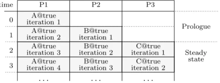
Fig. 5. Pipelined execution trace for the example of Fig. 4
f st(C) = 2
time P1 P2 P3
0 f st(A) = 0A@true f st(B) = 1B@true C@true
Fig. 6. Pipelined scheduling table (kernel) for the example of Fig. 4
processor being allocated in adjacent memory banks. This is why we only formalize here two correctness properties that will need attention in the following sections because pipelining transformations can affect them.
We say that two operations o1 and o2 are non-concurrent, denoted o1⊥o2, if either their
executions do not overlap in time (t (o1) + d(o1) ≤ t (o2) or t (o2) + d(o2) ≤ t (o1)), or if they
have exclusive guards (Guard(o1) ∧ Guard(o2) = false). With this notation, the following
correctness properties are assumed respected by input (non-pipelined) scheduling tables, and must be respected by the output (pipelined) ones:
Sequential processors. No two operations can use a processor at the same time. Formally,
for all o1, o2∈ O, if Res(o1) ∩ Res(o2) 6= ∅ then o1⊥o2.
No data races. If some memory cell m is written by o1 (m ∈ Out(o1)) and is used by o2
(m ∈ In(o2) ∪ Out(o2)), then o1⊥o2.
4. PIPELINING TECHNIQUE OVERVIEW 4.1. Pipelined scheduling tables
4.1.1. A simple example.For the example in Fig. 4, an execution where successive cycles do not overlap in time is clearly sub-optimal. Our objective is to allow the pipelined execution of Fig. 5, which ensures a maximal use of the computing resources.
In the pipelined execution, a new instance of operation A starts as soon as the previous one has completed, and the same is true for B and C. The first two time units of the execution are the prologue which fills the pipeline. In the steady state the pipeline is full and has a throughput of one computation cycle (of the non-pipelined system) per time unit. If the system is allowed to terminate, then completion is realized by the epilogue, not pictured in our example, which empties the pipeline.
We represent the pipelined system schedule using the pipelined scheduling table pictured in Fig. 6. Its length is 1, corresponding to the throughput of the pipelined system. The operation set contains the same operations A, B, and C, but there are significant changes. The start dates of B and C are now 0, as the 3 operations are started at the same time in each pipelined execution cycle. A non-pipelined execution cycle spans over several pipelined cycles, and each pipelined cycle starts one non-pipelined cycle.
To account for the prologue phase, where operations progressively start to execute, each operation is assigned a start index fst(o). If an operation o has fst(o) = n, it will first be executed in the pipelined cycle of index n (indices start at 0). Due to pipelining, the instance
y A C B D x P2 P1 M1 Bus M2 (a) (b)
Fig. 7. Example 2: Dataflow specification (a) and a bus-based implementation architecture (b)
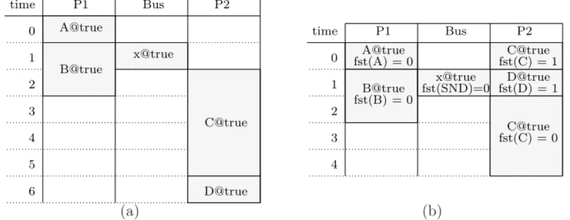
x@true 5 6 time 0 1 2 P1 A@true 3 Bus P2 B@true C@true D@true 4 x@true fst(C) = 0 fst(D) = 1 time 0 1 2 P1 3 Bus P2 4 C@true D@true A@true B@true C@true fst(A) = 0 fst(B) = 0 fst(SND)=0 fst(C) = 1 (a) (b)
Fig. 8. Example 2: Non-pipelined scheduling table produced by phase 1 of our technique (a) and pipelined table produced by phase 2 (b) for the example of Fig. 7
of o executed in the pipelined cycle m belongs to the non-pipelined cycle of index m− fst(o). For instance, operation C with fst(C) = 2 is first executed in the 3rd pipelined cycle (of
index 2), but belongs to the first non-pipelined cycle (of index 0).
4.1.2. Example 2: makespan vs. throughput optimization .The example of Fig. 7 showcases how the different optimization objectives of our technique lead to different scheduling results, when compared with existing software pipelining techniques.
The architecture is here more complex, involving a communication bus that connects the two identical processors. Communications over the bus are synthesized during the scheduling process, as needed. Note that the bus is modeled as a processor performing communication operations. This level of description, defined in Section 3.1, is accurate enough to support our pipelining algorithms. The makespan-optimizing scheduling algorithms used in phase 1 use more detailed architecture descriptions (outside the scope of this paper).
The functional specification is also more complex, involving parallelism and different durations for the computation and communication operations. The durations of A, B, C, and D on the two processors are respectively 1, 2, 4, and 1, and transmitting over the bus any of the data produced by A or C takes 1 time unit.
Fig. 8(a) provides the non-pipelined scheduling table produced for this example by the makespan-optimizing heuristics of [Potop-Butucaru et al. 2009]. Operations A and B have been allocated on processor P 1 and operations C and D have been allocated on P 2. One communication is needed to transmit data x from P 1 to P 2. The makespan is here equal to the table length, which is 7. The throughput is the inverse of the makespan (1/7).
When this scheduling table is given to our pipelining algorithm, the output is the pipelined scheduling table of Fig. 8(b). The makespan remains unchanged (7), but the table length is now 5, so the throughput is 1/5. Note that the execution of operation C starts in one
x@true P2 5 time 0 1 2 P1 3 Bus 4 C@true A@true B@true fst(A) = 0 fst(B) = 0 fst(SND)=0 fst(C) = 0 fst(D) = 1D@true fst(D) = 1 fst(x)=0 y@true fst(y)=1 time 0 1 2 P1 3 Bus A@true B@true fst(A) = 0 fst(B) = 0 P2 C@true fst(C) = 0 C@true D@true fst(C) = 1 x@true (a) (b)
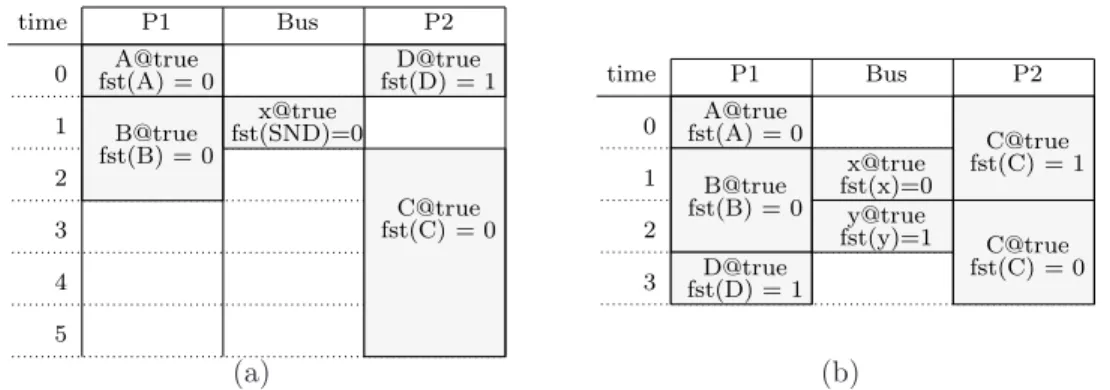
Fig. 9. Example 2: At left, the result of retiming the scheduling table of Fig. 8(a). At right, the result of directly applying throughput-optimizing modulo scheduling onto the specification of Fig. 7.
old m @(m=1) F1 @(m=2) F2 @(m=3) F3 ∆ @true init=1 @true MC m @true G m = 1 m= 2 m= 3 (a) (b)
Fig. 10. Example 3: Dataflow specification with conditional execution (a) and possible mode transitions (b)
pipelined execution cycle (at date 2), but ends in the next, at date 1. Thus, operation C has two reservations, one with fst(C) = 0, and one with fst(C) = 1.
Operations spanning over multiple execution cycles are not allowed in retiming-based techniques. Thus, if we apply retiming to the scheduling table of Fig. 8(a), we obtain the pipelined scheduling table of Fig. 9(a). For this example, the makespan is not changed, but the throughput is worse than the one produced by our technique (1/6).
But the most interesting comparison is between the output of our pipelining technique and the result of throughput-only optimization. Fig. 9(b) provides a pipelined scheduling table that has optimal throughput. In this table, operation D is executed by processor P 1, so that the bus must perform 2 communications. The throughput is better than in our case (1/4 vs. 1/5), but the makespan is worse (8 vs. 7), even though we chose a schedule with the best makespan among those with optimal throughput.
4.1.3. Example 3: Predication handling.To explain how predication is handled in our ap-proach, consider the example of Fig. 10. We only picture here the functional specification. As architecture, we consider two processors P 1 and P 2 connected to a shared memory M 1 (a 2-processor version of the architecture in Fig. 3(b)).
Example 3 introduces new constructs. First of all, it features a delay, labeled ∆. Delays are used in our data-flow formalism to represent the system state, and are a source of
inter-iteration dependences. Each delay has an initial value, which is given as output in the first
execution cycle, and then outputs at each cycle the value received as input at the previous cycle. The data-flow formalism, including delays, is formally defined in [Potop-Butucaru et al. 2009].
The functional specification also makes use of conditional (predicated) execution. Oper-ations F 1, F 2, and F 3 (of length 3, 2, and 1, respectively) are executed in those execution
MC@true time 0 1 P1 P2 2 3 4 5 6 F1 F2 F3 G G G @m=1 @m=2 @m=3 @m=3 @m=2 @m=1
Fig. 11. Example 3: non-pipelined scheduling table
cycles where the output m of operation M C equals respectively 1, 2, or 3. Operations M C and G are executed in all cycles.
The output m of operation M C (for mode computation) is used here to represent the
exe-cution mode of our application. This mode is recomputed in the beginning of each exeexe-cution
cycle by M C, based on the previous mode and on unspecified inputs directly acquired by M C. We assume that the application has only 3 possible modes (1, 2, and 3), and that transition between these modes is only posible as specified by the transitions of Fig. 10(b). This constraint is specified with a predicate over the inputs and outputs of operation M C. All data-flow operations can be associated such predicates, which will be used in the anal-yses of the next sections. Assuming that the input port of operation M C is called old m and that the output port is called m, the predicate associated to M C is:
(old m = m) or (old m = 1 and m = 2) or (old m = 2) or (old m = 3 and m = 2) This predicate states that either there is no state change (old m = m), or there is a transition from state 1 to state 2 (old m = 1 and m = 2), or that the old state is 2, so the new state can be any of the 3 (old m = 2), or that there is a transition from state 3 to state 2 (old m = 3 and m = 2).
We assume that operations M C, F 1, F 2, and F 3 are executed on processor P 1, and that G is executed on P 2. Under these conditions, one possible non-pipelined schedule produced by Phase 1 is the one pictured in Fig. 11. Note that this table features 3 conditional reservations for operation G, even if G does not have an execution condition in the data-flow graph. This allows G to start as early as possible in every given mode.
This table clearly features the reservation of the same resource, at the same time, by multiple operations. For instance, operations F 1, F 2, and F 3 share P 1 at date 1. Of course, each time this happens the operations must have exclusive predicates, meaning that there is no conflict at runtime.
Pipelining this table using the algorithms of the following sections produces the schedul-ing table of Fig. 12. The most interestschedul-ing aspect of this table is that the reservations
G@m=1,fst=1 and G@m=3,fst=0, which belong to different execution cycles of the
non-pipelined table, are allowed to overlap in time. This is possible because the dependency analysis of Section 5 determined that the two operations have exclusive execution condi-tions. In our case, this is due to the fact that m cannot change its value directly from 1 to 3 when moving from one non-pipelined cycle to the next.
When relations between execution conditions of operations belonging to different exe-cution cycles are not taken into account, the resulting pipelining is that of Fig. 13. Here, reservations for G cannot overlap in time if they have different fst values.
time 0 1 P1 P2 2 3 MC@true F3 @m=3 fst = 0 G @m=3 fst=1 G @m=2 fst = 0 F1 @m=1 fst = 0 F2 @m=2 fst = 0 G @m=1 fst=1 G @m=2 fst=1 G @m=3 fst = 0
Fig. 12. Example 3: Pipelined scheduling table pro-duced by our technique
time 0 1 P1 P2 2 3 4 fst=1 @m=2 MC@true @m=1 fst=1 G G F1 @m=1 fst=0 F2 @m=2 fst=0 F3 @m=3 fst=0 G @m=2 fst=0 G @m=1 fst=0 G @m=3 fst=0
Fig. 13. Example 3: Pipelined scheduling table where inter-cycle execution condition analysis has not been used to improve sharing.
The current implementation of our algorithms can only analyze predicates with Boolean arguments. Thus, our 3-valued mode variable m needs re-encoding with 2 Boolean variables. In other words, in the version of Example 3 that can be processed by our tool, the operation M C actually has 2 Boolean inputs and 2 Boolean outputs, and the predicate above is defined using these 4 variables.
4.2. Construction of the pipelined scheduling table
The prologues of our pipelined executions are obtained by incremental activation of the steady state operations, as specified by the fst indices (this is a classical feature of modulo scheduling pipelining approaches). Then, the pipelined scheduling table can be fully built using Algorithm 1 starting from the non-pipelined table and from the pipelined initiation interval. The algorithm first determines the start index and new start date of each operation by folding the non-pipelined table onto the new period. Algorithm AssembleSchedule then determines which memory cells need to be replicated due to pipelining, using the technique provided in Section 4.4.
Input: S : non-pipelined scheduling table b
p : pipelined initiation interval Output: bS : pipelined schedule table
for all o in O do
fst(o) := ⌊t(o)bp ⌋
bt(o) := t(o) − fst(o) ∗ bp end for
b
S := AssembleSchedule(S, bp, fst, bt)
Algorithm 1: BuildSchedule
4.3. Dependency graph and maximal throughput
The period of the pipelined system is determined by the data dependences between suc-cessive execution cycles and by the resource constraints. If we follow the classification of [Hennessy and Patterson 2007], we are interested here in true data dependences, and not in name dependences such as anti-dependences and output dependences. A true data depen-dency exists between two operations when one uses as input the value computed by the other. Name dependencies are related to the reuse of variables, and can be eliminated by variable renaming. For instance, consider the following C code fragment:
Here, there is a true data dependence (on variable y) between statements 2 and 3. There is also an anti-dependence (on variable y) between statements 1 and 2 (they cannot be re-ordered without changing the result of the execution). Renaming variable y in statements 2 and 3 removes this anti-dependence and allows re-ordering of statements 1 and 2:
x := y + z; y2:= 10; z := y2;
In our case, not needing the analysis of name dependences is due to the use of the rotating register files (detailed in Section 4.4) which remove anti-dependences, and to the fact that output dependences are not semantically meaningful in our systems whose execution is meant to be infinite.
We represent data dependences as a Data Dependency Graph (DDG) – a formalism that is classical in software pipelining based on modulo scheduling techniques[Allan et al. 1995]. In this section we define DDGs and we explain how the new period is computed from them. The computation of DDGs is detailed in Section 5.
Given a scheduling table S =< p, O, Init >, the DDG associated to S is a directed graph DG =< O, V > where V ⊆ O × O × N. Ideally, V contains all the triples (o1, o2, n) such
that there exists an execution of the scheduling table and a computation cycle k such that operation o1 is executed in cycle k, operation o2 is executed in cycle k + n, and o2 uses
a value produced by o1. In practice, any V including all the arcs defined above (any
over-approximation) will be acceptable, leading to correct (but possibly sub-optimal) pipelinings. The DDG represents all possible dependences between operations, both inside a compu-tation cycle (when n = 0) and between successive cycles at distance n ≥ 1. Given the static scheduling approach, with fixed dates for each operation, the pipelined scheduling table must respect unconditionally all these dependences.
For each operation o ∈ O, we denote with tn(o) the date where operation o is executed
in cycle n, if its guard is true. By construction, we have tn(o) = t (o) + n ∗ p. In the
pipelined scheduling table of period bp, this date is changed to btn(o) = t (o) + n ∗ bp. Then,
for all (o1, o2, n) ∈ V and k ≥ 0, the pipelined scheduling table must satisfy btk+n(o2) ≥
btk(o1) + d(o1), which implies:
b
p ≥ max
(o1,o2,n)∈V,n6=0
⌈t (o1) + d(o1) − t (o2)
n ⌉
Our objective is to build pipelined scheduling tables satisfying this lower bound constraint and which are well-formed in the sense of Section 3.3.
4.4. Memory management issues
Our pipelining technique allows multiple instances of a given variable, belonging to succes-sive non-pipelined execution cycles, to be simultaneously live. For instance, in the example of Figures 4 and 5 both A and B use memory cell v1 at each cycle. In the pipelined table,
A and B work in parallel, so they must use two different copies of v1. In other words, we
must provide an implementation of the expanded virtual registers of [Rau 1996].
The traditional software solution to this problem is the modulo variable expansion of [Lam 1988]. However, this solution requires loop unrolling, which would increase the size of our scheduling tables. Instead, we rely on a purely software implementation of rotating
register files [Rau et al. 1992], which requires no loop unrolling, nor special hardware
sup-port. Our implementation of rotating register files includes an extension for identifying the good register to read in the presence of predication. To our best knowledge, this extension (detailed in Section 4.4.2) is an original contribution.
4.4.1. Rotating register files for stateless systems. Assuming that bS is the pipelined version of S, we denote with max par = ⌈len(S)/len( bS)⌉ the maximal number of
simultaneously-active computation cycles of the pipelined scheduling table. Note that max par = 1 + maxo∈Ofst(o).
In the example of Figures 4 and 5 we must use two different copies of v1. We will say that
the replication factor of v1is rep(v1) = 2. Each memory cell v is assigned its own replication
factor, which must allow concurrent non-pipelined execution cycles using different copies of v to work without interference. Obviously, we can bound rep(v) by max par. We use a tighter margin, based on the observation that most variables (memory cells) have a limited lifetime inside a non-pipelined execution cycle. We set rep(v) = 1 + lst(v) − fst(v), where:
fst(v) = minv∈In(o)∪Out(o)fst(o) lst(v) = maxv∈In(o)∪Out(o)fst(o)
Through replication, each memory cell v of the non-pipelined scheduling table is replaced by rep(v) memory cells, allocated on the same memory block as v, and organized in an array v, whose elements are v[0], . . . , v[rep(v)−1]. These new memory cells are allocated cyclically, in a static fashion, to the successive non-pipelined cycles. More precisely, the non-pipelined cycle of index n is assigned the replicas v[n mod rep(v)] for all v. The computation of rep(v) ensures that if n1 and n2 are equal modulo rep(v), but n1 6= n2, then computation cycles
n1 and n2cannot access v at the same time.
To exploit replication, the code generation scheme must be modified by replacing v with v[(cid − fst(o)) mod rep(v)] in the input and output parameter lists of every operation o that uses v. Here, cid is the index of the current pipelined cycle. It is represented in the generated code by an integer. When execution starts, cid is initialized with 0. At the start of each subsequent pipelined cycle, it is updated to (cid + 1) mod R, where R is the least common multiple of all the values rep(v).
This simple implementation of rotating register files allows code generation for systems where no information is passed from one non-pipelined execution cycle to the next (no inter-cycle dependences). Such systems, such as the example in Figures 4 and 5, are also called state-less.
4.4.2. Extension to stateful predicated systems. In stateful systems, one (non-pipelined) ex-ecution cycle may use values produced in previous exex-ecution cycles. In these cases, code generation is more complicated, because an execution cycle must access memory cells that are not its own.
For certain classes of applications (such as systems without conditional control or affine loop nests), the cells to access can be statically identified by offsets with respect to the current execution cycle. For instance, the M C mode change function of Example 3 (Sec-tion 4.1.3) always reads the variable m produced in the previous execu(Sec-tion cycle.
But in the general case, in the presence of predicated execution, it is impossible to stat-ically determine which cell to read, as the value may have been produced at an arbitrary distance in the past. This is the case if, for instance, the data production operation is itself predicated. One solution to this problem is to allow the copying of one memory cell onto another in the beginning of pipelined cycles. But we cannot accept this solution due to the nature of our data, which can be large tables for which copying implies large timing penalties.
Instead, we modify the rotating register file as follows: Storage is still ensured by the v circular buffer, which has the same length. However, its elements are not directly addressed through the modulo counter (cid − fst(v)) mod rep(v) used above. Instead, this counter points in an array srcv whose cells are integer indices pointing towards cells of v. This
allows operations from several non-pipelined execution cycles (with different cid and fst(o)) to read the same cell of v, eliminating the need for copying.
The full implementation of our register file requires two more variables: An integer nextv
and an array of Booleans write flagvof length rep(v). Since v is no longer directly addressed
by pointing to the cell where a newly-produced value can be stored next. One cell of v is allocated (and nextv incremented) whenever a non-pipelined execution cycle writes v for
the first time. Subsequent writes of v from the same non-pipelined cycle use the already allocated cell. Determining whether a write is the first from a given non-pipelined execution cycle is realized using the flags of write flagv. Note that the use of these flags is not needed
when a variable can be written at most once per execution cycle. This is often the case for code used in embedded systems design, such as the output of the Scade language compiler, or the output of the makespan-optimizing scheduling tool used for evaluation. If a given execution cycle does not write v, then it must read the same memory cell of nextvthat was
used by the previous execution cycle.
The resulting code generation scheme is precisely described by the following rules: (1) At application start, for every every memory cell (variable) v of the initial specification,
srcv[0], write flagv[0], nextv are initialized respectively with 0, false, and 1. If Init(v) 6=
nil then v[0] (instead of v) is initialized with this value.
(2) At the start of each pipelined cycle, for memory cell (variable) v of the initial scheduling table, assign to srcv[(cid − fst(v)) mod rep(v)] the value of srcv[(cid − fst(v) − 1) mod
rep(v)], and set write flagv[(cid − fst(v)) mod rep(v)] to false.
(3) In all operations o replace each input and output cell v with v[srcv[(cid − fst(o)) mod
rep(v)]]. The same must be done for all cells used in the computation of execution
conditions.
(4) When an operation o has v as an output parameter, then some code must be added before the operation (inside its execution condition). There are two cases. If v is not an input parameter of o, then the code is the following:
1: if not write flagv[(cid − fst(o)) mod rep(v)] then
2: write flagv[(cid − fst(o)) mod rep(v)] = true
3: srcv[(cid − fst(o)) mod rep(v)] = nextv
4: nextv= (nextv+ 1) mod rep(v)
5: end if
If v is also an input parameter of o, then only line 2 is needed from the previous code. 4.4.3. Accounting for book keeping costs. The software implementation of the rotating register files induces a timing overhead of its own. This overhead is formed of two components: — Per operation costs, which can be conservatively accounted for in the WCET of the
operations, as it is provided to the Phase 1 of our scheduling flow:
— For each operation and for each input and output parameter, the cost of the indirection of point (3) above. This amounts to 2 indirections, one addition, and one modulo operation.
— For each operation and for each output parameter, the cost of the bookkeeping oper-ations defined at point (4) above.
— Per iteration costs, associated to point (2) above, and which must be added to the length of the pipelined scheduling table. This amounts to updating the srcv and write flagv
data structures for all v. These costs are also bounded and can be accounted for with worst-case figures in Phase 1.
One important remark here is that our operations are large-grain tasks, meaning that these costs are often considered negligible, even for hard real-time applications.
The use of rotating registers also results in memory usage overheads. These overheads come from the replication of memory cells and from the pointer arrays srcv which must be
stored on the same memory bank as v for all memory cell v. We will assume that the cost of src is negligible, and only be concerned with the cost of replication, especially for large data.
time 0 P2 P1 P3 1 2 A@true B@true C@true D@true 3
Fig. 14. Dependency analysis example, non-pipelined
1
time P1 P2 P3
0 f st(A) = 0A@true C@true B@true
f st(D) = 1D@true f st(B) = 0
f st(C) = 1
Fig. 15. Dependency analysis example, pipelined
If the replication of a large piece of data is a concern, then we can prohibit it altogether by requiring that all accesses to that memory cell are sequenced. This is done by adding a “sequencer” processor to the architecture model, and requiring all accesses to that memory cell to use the sequencer processor (this requires modifications to both the architecture and the functional specification). The introduction of sequencers may limit the efficiency of our pipelining algorithms. However, being able to target specific memory cells means that we can limit efficiency loss to what is really necessary on our memory-constrained embedded platforms. This simple approach satisfies our current needs.
5. DEPENDENCY ANALYSIS AND MAIN ROUTINE
Dependency analysis is a mature discipline, and powerful algorithms have been used in practice for decades [Muchnick 1997]. However, previous research on inter-iteration depen-dency analysis has mostly focused on exploiting the regularity of code such as affine loop nests. To the best of our knowledge, existing algorithms are unable to analyze specifications such as our Example 3 (Section 4.1.3) with the precision we seek. Doing this requires that inter-iteration dependency analysis deals with data-dependent mode changes (which are a common feature in embedded systems design).
Performing our precise inter-iteration dependency analysis requires the (potentially infi-nite) unrolling of the non-pipelined scheduling table. But our specific pipelining technique allows us to bound the unrolling, and thus limit the complexity of dependency analysis. By comparison, existing pipelining and predicate-aware scheduling techniques either assume that the dependency graph is fully generated before starting the pipelining algorithm [Rau and Glaeser 1981], or use the predicates for the analysis of a single cycle[Warter et al. 1993]. The core of our dependency analysis consists in the lines 1-10 of Algorithm 3, which act as a driver for Algorithm 2. The remainder of Algorithm 3 uses DDG-derived information to drive the pipelining routine (Algorithm 1).
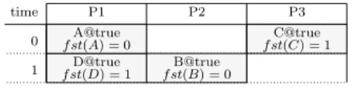
Both the data dependency analysis and pipelining driver take as input a flag that chooses between two pipelining modes with different complexities and capabilities. To understand the difference, consider the non-pipelined scheduling table of Fig. 14. Resource P1 has an
idle period between operations A and D where a new instance of A can be started. However, to preserve a periodic execution model, A should not be restarted just after its first instance (at date 1). Indeed, this would imply a pipelined throughput of 1, but the fourth instance of A cannot be started at date 3 (only at date 6). The correct pipelining starts A at date 2, and results in the pipelined scheduling table of Fig. 15.
Determining if the reuse of idle spaces between operations is possible consists in deter-mining the smallest integer n greater than the lower bound of Section 4.3, smaller than the length of the initial table, and such that a well-formed pipelined table of length n can be constructed. This computation is performed by lines 14-19 of Algorithm 3. We do not provide here the code of function WellFormed, which checks the respect of the well-formed properties of Section 3.3.
This complex computation can be avoided when idle spaces between two operations are excluded from use at pipelining time. This can be done by creating a dependency between
any two operations of successive cycles that use a same resource and have non-exclusive execution conditions. In this case, the pipelined system period is exactly the lower bound of Section 4.3, and the output scheduling table is produced with a single call to Algorithm 1 (BuildSchedule) in line 12 of Algorithm 3. Of course, Algorithm 2 needs to consider (in lines 10-16) the extra dependences.
Excluding the idle spaces from pipelining also has the advantage of supporting a sporadic execution model. In sporadic systems the successive computation cycles can be executed with the maximal throughput specified by the pipelined table, but can also be triggered arbitrarily less often, for instance to tolerate timing variations, or to minimize power con-sumption in systems where the demand for computing power varies. On the contrary, using the idle spaces during pipelining imposes synchronization constraints between successive execution cycles. For instance, in the pipelined system of Fig. 15, the computation cycle of index n cannot complete before operation A of cycle n + 1 is completed.
The remainder of this section details the dependency analysis phase. The output of this analysis is the lower bound defined in Section 4.3, computed as period lbound. The analysis is organized around the repeat loop which incrementally computes, for cycle ≥ 1, the DDG dependences of the type (o1, o2, cycle). The computation of the DDG is not complete: We
bound it using a loop termination condition derived from our knowledge of the pipelining algorithm. This condition is based on the observation that if period lbound ∗ k ≥ len(S) then execution cycles n and n + k cannot overlap in time (for all n).
The DDG computation works by incrementally unrolling the non-pipelined scheduling table. At each unrolling step, the result is put in the SSA4-like data structureS that allows
the computation of (an over-approximation of) the dependency set. Unrolling is done by annotating each instance of an operation o with the cycle n in which it has been instantiated. The notation is on. Putting in SSA-like form is based on splitting each memory cell v into
one version per operation instance producing it (vn
o, if v ∈ Out(o)), and one version for the
initial value (vinit). Annotation and variable splitting is done on a per-cycle basis by the
Annotate routine (not provided here) which changes for each operation o its name to on,
and replaces Out(o) with {vn
o | v ∈ Out(o)} (n is here the cycle index parameter). Instances
of S produced by Annotate are then assembled into S by the Concat function which simply adds to the date of every operation in the second argument the length of its first argument. Recall that we are only interested in dependences between operations in different cycles. Then, in each call to Algorithm 2 we determine the dependences between operations of cycle 0 and operations of cycle n, where n is the current cycle. To determine them, we rely on a symbolic execution of the newly-added part of S, i.e. the operations ok with k = n.
Symbolic execution is done through a traversal of list l, which contains all operation start and end events of S, and therefore S, ordered by increasing date. For each operation o of S, l contains two elements labeled start(o) and end(o). The list is ordered by increasing event date using the convention that the date of start(o) is t (o), and the date of end(o) is
t (o) + d(o). Moreover, if start(o) and end(o′) have the same date, the start(o) event comes
first in the list.
At each point of the symbolic execution, the data structure curr identifies the possible producers of each memory cell. For each cell v of the initial table, curr(v) is a set of pairs w@C, where w is a version of v of the form vk
o or vinit, and C is a predicate over memory
cell versions. In the pair w@C, C gives the condition on which the value of v is the one corresponding to its version w at the condidered point in the symbolic simulation. Intuitively, if vk
o@C ∈ curr(v), and we symbolically execute cycle n, then C gives the condition under
which in any real execution of the system v holds the value produced by o, n − k cycles before. The predicates of the elements in curr(v) provide a partition of true. Initially, curr(v)
4
Inputs: S : non-pipelined scheduling table l : the list of events of S
n : integer (cycle index)
fast pipelining flag : boolean
InputOutputs: S : annotated scheduling table curr : current variable assignments
DDG : Data Dependency Graph
1: S := Concat(S, Annotate(S, n)) 2: while l not empty do
3: e := head(l) ; l := tail(l) 4: if e = start(o) then 5: Replace Guard(on) by W wi@Ci∈curr(vi),i=1,k (C1∧ . . . ∧ Ck) ∧ go(w1, . . . , wk) where Guard(o) = go(v1, . . . , vk).
6: for all p operation in S, u ∈ Out(p), v ∈ In(o) do
7: if u0
p@C ∈ curr(v) and ¬Exclusive(C, Guard(on)) then
8: DDG := DDG ∪ {(p, o, n)}
9: end if
10: if fast pipelining flag then 11: if Res(o) ∩ Res(p) 6= ∅ then
12: if ¬Exclusive(Guard(on), Guard(p0)) then
13: DDG := DDG ∪ {(p, o, n)} 14: end if 15: end if 16: end if 17: end for 18: else 19: /* e = end(o) */ 20: for all v ∈ Out(o) do 21: new curr := {vn
o@Guard(on)}
22: for all vkp@C ∈ curr(v) do
23: C′ := C ∧ ¬Guard(on)
24: if ¬Exclusive(C, Guard(on)) then 25: new curr := new curr ∪ {vk
p@C′}
26: end if
27: end for
28: curr(v) := new curr
29: end for
30: end if 31: end while
Algorithm 2: DependencyAnalysisStep
is set to {vinit@true} for all v. This is changed by Algorithm 2 (lines 20-29), and by the
call to InitCurr in Algorithm 3. We do not provide this last function, which performs the symbolic execution of the nodes ofS annotated with 0. Its code is virtually identical to that of Algorithm 2, lines 1 and 6-17 being excluded.
At each operation start step of the symbolic execution, curr allows us to complete the SSA transformation by recomputing the guard of the current operation over the split variables (line 5 of Algorithm 2). In turn, this allows the computation of the dependences (lines 6-17). Guard comparisons are translated into predicates that are analyzed by a SAT solver. This translation into predicates also considers the predicates relating inputs and outputs of the
data-flow operations, as intuitively explained in Section 4.1.3. The translation and the call to SAT are realized by the Exclusive function, not provided here.
Input: S : non-pipelined schedule table
fast pipelining flag : boolean
Output: bS : pipelined schedule table 1: l := BuildEventList(S) 2: period lbound := 0 3: cycle := 0 4: S := Annotate(S, cycle) 5: curr := InitCurr(S) 6: repeat 7: cycle:=cycle + 1 8: (S, curr, DDG) := DependencyAnalysisStep(S, l,
cycle,fast pipelining flag, S, curr, DDG)
9: period lbound := max(period lbound, max(o1,o2,cycle)∈DDG⌈
t(o1)+d(o1)−t(o2) cycle ⌉ )
10: until period lbound ∗ cycle ≥ len(S) 11: if fast pipelining flag then
12: S := BuildSchedule(S, period lbound)b 13: else
14: for new period := period lbound to len(S) do 15: S := BuildSchedule(S, new period)b
16: if WellFormed(bS) then 17: goto 21 18: end if 19: end for 20: end if 21: return Algorithm 3: PipeliningDriver 5.1. Complexity considerations
The pipelining algorithm per se consists in Algorithm 1 and its driver (lines 11-20 of Al-gorithm 3). The complexity of AlAl-gorithm 1 is linear in the number of operations in the scheduling table. As explained above, the complexity of the driver routine (lines 11-20 of Algorithm 3) depends on the value of fast pipelining flag. When it is set to true, a single call to Algorithm 1 is performed. When it is set to false, the number of calls to Algorithm 1 is bounded by len(S).
In our experiments, fast pipelining flag is set for all examples, and the pipelining time is negligible.
But the main source of theoretical complexity in our pipelining technique is hidden in the dependency analysis implemented by Algorithm 2 and its driver (lines 1-10 or Algorithm 3). In Algorithm 3, the number of iterations in the construction of the DDG is up-bounded by len(S) (which can be large). Algorithm 2 is polynomial (quadratic) in the number of operations of the scheduling table, but involves comparisons of predicates with Boolean arguments (instances of the Boolean satisfiability problem SAT). Hence, our algorithm is overall NP-complete.
In practice, however, DDG construction time is negligible for all examples, real-life and synthesized. There are 2 reasons to this:
— In examples featuring predicated execution, the predicates remain simple, so that SAT instances are solved in negligible time.
— The number of iterations in the construction of the DDG is bounded by the condition in line 10 of Algorithm 3. In our experiments the maximal number of iterations is 2. 6. EXPERIMENTAL RESULTS
We have implemented our pipelining algorithms in a prototype tool. We have integrated this tool with an existing makespan-optimizing scheduling tool[Potop-Butucaru et al. 2009] to form the full, two-phase flow of Fig. 1.
We have applied the resulting toolchain on 4 significant, real-life examples from the testbench of the SynDEx scheduling tool[Grandpierre and Sorel 2003]. As no standard benchmarks are available in the embedded world, we have also applied our toolchain on a larger number of automatically synthesized dataflow graphs.
Our objective was to evaluate both the standalone pipelining algorithm, and the two-phase flow as a whole. Comparing with optimal scheduling results was not possible.5Instead,
we rely on comparisons with existing scheduling and pipelining heuristics:
(1) To evaluate the standalone algorithm, we measure the throughput gains obtained through pipelining, by comparing the initiation intervals of our examples before and after pipelining.
(2) To evaluate the two-phase flow as a whole, we compare its output to the output of a clas-sical throughput-optimizing software pipelining technique, namely the FRLC algorithm of [Wang and Eisenbeis 1993].
The testbench. The largest examples of our testbench (“cycab” and “robucar”) are
em-bedded control applications for the CyCab electric car [Pradalier et al. 2005]. The other two applications are an adaptive equalizer and a simplified model of an automotive knock control application [Andr´e et al. 2007].
We have used a script to automatically synthesize 30 examples (of which the first 10 are also presented individually in the result tables). For each example, synthesis is done as follows: We start with a graph containing only one data-flow node and no dependency. We apply a fixed number of expansion steps (3 steps for the examples in Fig. 17). At every step, each node is replaced with either a parallel or a sequential composition of newly-created nodes. The sequential and parallel choices are equiprobable. The number of nodes generated through expansion is chosen with a uniform distribution in the interval [1..5]. Dependences are also generated randomly at each step, and all previously-existing dependences are pre-served. We implement these data-flow graphs on an architecture containing 5 processors and one broadcast bus. To model the fact that the architecture is not homogenous, the durations
5
Providing optimal solutions to our scheduling problem proved intractable even for small systems with 10 blocks and 3 processors.
Example size Scheduling table length (initiation interval) example blocks processors initial pipelined gain
(makespan) (kernel)
cycab 40 3 1482 1083 27%
robucar 84 3 1093 1053 8%
ega 67 2 84 79 6%
knock 5 2 6 3 50%
Fig. 16. Pipelining gains for the real-life applications. Durations are in time units whose actual real-time length depends on the application (e.g. milliseconds).