Quality Assessment of the French OpenStreetMap Dataset

HAL Id: hal-02320425

https://hal.archives-ouvertes.fr/hal-02320425

Submitted on 18 Oct 2019

HAL is a multi-disciplinary open access archive for the deposit and dissemination of sci-entific research documents, whether they are pub-lished or not. The documents may come from teaching and research institutions in France or abroad, or from public or private research centers.

L’archive ouverte pluridisciplinaire HAL, est destinée au dépôt et à la diffusion de documents scientifiques de niveau recherche, publiés ou non, émanant des établissements d’enseignement et de recherche français ou étrangers, des laboratoires publics ou privés.

Dataset

Jean-François Girres, Guillaume Touya

To cite this version:

Jean-François Girres, Guillaume Touya. Quality Assessment of the French OpenStreetMap Dataset. Transactions in GIS, Wiley, 2010, 14 (4), pp.435-459. �10.1111/j.1467-9671.2010.01203.x�. �hal-02320425�

Quality Assessment of the French OpenStreetMap dataset

Jean-François Girres1, Guillaume Touya1

1

COGIT Laboratory, IGN, 73 Avenue de Paris, 94165 Saint-Mandé, France

ABSTRACT. The concept of Volunteered Geographic Information (VGI) has recently emerged from the new Web 2.0 technologies. The OpenStreetMap project is currently the most significant example of a system based on VGI. It aims at producing free vector geographic databases using contributions from Internet users. Spatial data quality becomes a key consideration in this context of freely downloadable geographic databases. This article studies the quality of French OpenStreetMap data. It extends the work of Haklay to France, provides a larger set of spatial data quality element assessments (i.e. geometric, attribute, semantic and temporal accuracy, logical consistency, completeness, lineage, and usage), and uses different methods of quality control. The outcome of the study raises questions such as the heterogeneity of processes, scales of production, and the compliance to standardized and accepted specifications. In order to improve data quality, a balance has to be struck between the contributors’ freedom and their respect of specifications. The development of appropriate solutions to provide this balance is an important research issue in the domain of user-generated content. KEYWORDS: OpenStreetMap, spatial data quality, VGI, specifications

1. Introduction

With the advent of the current Web 2.0, contributors do not just look for content but are also creating it themselves, as showing the success of Facebook, MySpace, YouTube or forums. This new phenomenon generates new methods of production that Tapscott and Williams (2007) describe as the crowdsourcing, which consists in using the expertise of a large number of users to perform tasks at a lower cost. At the same time, the success of open source

software is extended by the emergence of open databases that can be used more or less freely depending on the type of license. Thus, some new spatial data producers as local

administrations (Touya, 2004) prefer to make an entire community benefit from the data they produce rather than keep data for private use. Together with the democratisation of GPS, these two phenomena meet up today turning everyone into a sensor of geographic

information, able to provide a contributively created geographic information or Volunteered Geographic Information (VGI) (Goodchild, 2007). That is what Sui (2008) called the

wikification of geographic information.

In this context, the rapid development of the OpenStreetMap project (OSM), born in 2004 in England, is not surprising (http://www.openstreetmap.org). Each project member is invited to submit data acquired mainly by GPS. It is then available mapped on the website like in cartography sites as GoogleMaps or the Geoportals. But above all OpenStreetMap data are freely downloadable in vector format. The project, which was originally limited to English roads, has spread around the world, and allows to capture topographic databases. Given the possible applications of spatial vector databases (mapping, geographic analysis, urban planning or risk prevention), the question of the quality of such data should be asked,

including comparison with institutional geographic databases, as those of the French National Mapping Agency (Institut Geographique National, IGN). Thus, Haklay (2009) suggested comparing British OSM data with those of the Ordnance Survey, the English national mapping agency. The objective of the work presented in this paper is to extend this work to French data taking into account different aspects of quality of a geographic database, and to analyse the OpenSteetMap’s production model compared to those of institutional databases.

The objective of this work is also to experiment quality control methods and tools for a geographic database.

The second part of this section describes more precisely the OSM project with its data, methods, objectives and its applications. The third part proposes a study of OSM data quality compared to the BD TOPO ® from IGN, regarding all aspects of spatial data quality. Then, the fourth section puts into perspective the question of databases production models. The fifth section discusses the definition of spatial data quality regarding the preceding analysis. Finally, the article ends with a conclusion and further research.

2. What is OpenStreetMap?

OpenStreetMap (OSM) is a collaborative project like Wikipedia, started in England in 2004 by Steve Coast. The aim of OSM is to create and provide free geographic data. The project aims to compensate the lack of free data because geographic data, even freely available, are provided with licenses restricting the use of information and the creativity according to project leaders. The data are distributed under the license “Creative Commons Attribution-ShareAlike 2.0 license”. This license allows using the data completely freely, in condition to distribute any derived data under the same license. For instance, corrected OSM data can not be sold.

Data stored in OSM by contributors of the project are modelled and stored in tagged geometric primitives (see 3.2). For example, a road is a polyline with tags highway =

"primary", oneway = "no" and name = "N10". Geometric primitives are of three types: points, paths (polylines) and relationships (linking points and paths with tags) that are not really geometric primitives. The surfaces are represented by closed paths. There are quite precise specifications listing the accepted tags and fields of values (Figure 1). A contributor can submit a new tag or a new value, that can be added to the specifications after a vote. Even if it is not advised, the contributor is free to use tags and values outside of these specifications. To facilitate the work of the contributor, there are also information files showing how to tag a given situation: in the Figure 2, the situation of the image is modelled by 3 items (2 roads and a tramway line). Data are available from any area specified for export in a specific XML based format. It has to be translated if anyone wishes to use the data in another application.

Figure 1. Preview of the specifications (in French) of the tag "highway".

Data is captured using a GIS software adapted to OSM data with editing functions to create OSM geometric primitives and tag them. Different software exist to edit and capture OSM data (Potlatch ®, JOSM ®, Merkaartor ®). In such software, data can be created directly but come generally from free sources like personal GPS tracks, satellite imagery or as cadastral data that have been made available for the project.

Figure 2. Preview of an information leaflet to tag situations. Here, a tramway line.

OSM applications currently aim to foster mapping creativity of potential contributors of geographic data. Thus, there are various sites proposing OSM data as CloudMade (route calculation) or GeoFabrik (which provides OSM data in shapefile for example). Allan (2008) offers maps suitable for cyclists.

3. Quality assessment of OpenStreetMap data in France

3.1. Quality of a geographic database

To assess the quality of spatial data provided by OpenStreetMap, we use quality control methods in a geographic database. For the geometric precision and some other aspects, we use as a reference dataset, the BD Topo ® Large Scale Referential (RGE) from IGN. Vauglin (1997) differentiates several components in the description of geographic database quality. We propose those retained by the ISO norm (Kresse and Fadaie, 2003):

- Geometric accuracy: assesses the positioning and geometries resolution from the ground reality.

- Attribute accuracy: assesses the accuracy of attributes captured according to the specifications of the database.

- Completeness: evaluates if all data are present in the database.

- Logical consistency: assesses the degree of internal consistency as modelling rules and specifications (including respect of integrity constraints (Servigne et al, 2000)).

- Semantic accuracy: assesses if the semantics carried by the objects correspond to the real world.

- Currentness: evaluates the actuality of the database relative to changes in the real world. - Lineage: concerns the lineage of objects, their capture and their evolution.

- Usage: evaluates how well the database fits for the use that will be made.

3.2. Comparison of data models

Institutional geographic databases are structured in classes, attributes and relationships (Goodchild, 1992). An object of a geographic database belongs therefore to a class, for example road segment, and has values for different attributes of the class, such as "Highway" for the attribute nature and "20m" for the attribute width. The BD TOPO ® IGN is composed of thirty classes divided into different themes such as hydrography, buildings or transportation systems.

As stated in section 2, OMS data follow a different model rather used in the management of Internet resources, the Resource Description Framework (RDF) defined in Manola and Miller (2004). Information is modelled as a triple (resource, property, value). In the case of OSM, the resource is a geometric primitive with coordinates, the property is a tag and the value is a value of the tag. The triple follow the form: (point(x, y); highway; primary). This RDF information is represented in XML as in (Figure 3). Compared to a conventional structure in classes and attributes, RDF allows the easy integration of not obvious objects to identify in classes but on which we know certain properties. Lemmens (2006) explains that the RDF is particularly effective if it is coupled with a RDF Schema model that describes resources and properties with a vocabulary. In the case of OSM, specifications are not as structured as in a RDFS model.

Figure 3. Example of a geometric primitive (a point) tagged in RDF in the XML export format of OSM.

The RDF structure can pose several problems. It is quite complex to translate data into RDF classes and attributes. Several solutions are possible to switch from one to another, but the translation into classes inevitably generate losses on the tag information and the number of classes is not easy to decide. For example, tags that characterise highway roads may include points, lines, or surfaces and the separation into classes is not clear. The reverse transition is automatic (Lemmens, 2006). Another problem concerns identification of real world objects. The ideal way would be to carry a unique identifier on the real world entities, or on an object. In the case of OSM, identifiers refer to the geometric primitives which generates difficulties to manage and update databases.

Nevertheless, structuring geographic data in a RDF format can also prove interesting. Goodwin et al (2008) translated Ordnance Survey Administrative database in RDF to facilitate interoperability but using an ontology to formalise properties contrary to OSM. Goodwin et al (2008) also noticed that topology relations explicitly stored in RDF allowed good querying performance.

<node id="25213726" lat="43.3020693" lon="-0.3420626" version="3" changeset="52741" user="betsubetsu" uid="43565" visible="true" timestamp="2008-06-04T16:10:13Z">

<tag k="name" v="Station Shell"/> <tag k="postal_code" v="64000"/> <tag k="created_by" v="Potlatch 0.9c"/> <tag k="amenity" v="fuel"/>

<tag k="fuel_lpg" v="yes"/> <tag k="is_in" v="PAU"/>

<tag k="source" v="stations.gpl.online.fr"/>

<tag k="address" v="65, Avenue Maréchal Leclerc"/> </node>

3.3. Geometric Accuracy

To estimate geometric accuracy, comparisons are realised between the OSM data (data sets to compare) and BD TOPO ® the reference datasets. BD TOPO® is a metric resolution database which means that positional accuracy is around 1 meter but varies among themes (some are more precise than others). “Homologous” objects are selected and matched manually to avoid errors related to an automatic process. Differences in position are then computed on each pair of homologous objects. A specific application is developed in Java, based on the GeOxygene library (Bucher et al, 2009).

3.3.1. Points primitives

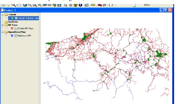
The comparison test of point objects is realised on road intersections from road layers of the two databases in the region of Hendaye. Pre-treatment using a topological map from

GeOxygene allows generating nodes, corresponding to road intersections. A sample of 207 pairs of homologous point objects is achieved by manual selection, trying as best as possible to cover the entire study area (Figure 4).

Figure 4. Localization (in green) of the 207 pairs of homologous point objects

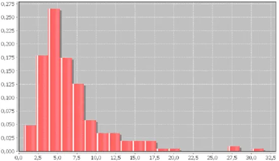
For each pair of selected point objects, Euclidean distance is used to generate a distance distribution drawn in Figure 5 and summarised in Table 1. The distribution of positional differences presented in Figure 5 shows a concentration between 2.5 and 10 meters. The average positional difference, computed from the sample, is about 6.65 meters. This distance is close to the average difference of about 6 meters observed between OSM and Ordnance Survey datasets according to Haklay (2009). Important differences - the maximum distance recorded is 31.58 meters - are relatively marginal. They are certainly due to errors of capture by the operator. This first result already shows a key property of OSM namely the

heterogeneity of data quality, highlighted by the important standard deviation that is three times more important that the reference precision (1.5 m).

Figure 5. Distribution of Euclidean distances from the sample of road intersections

Table 1. Statistics computed from Euclidean distances between crossroads.

3.3.2. Linear primitives

To characterise positional differences between linear objects, two distances are used: the Hausdorff distance and the average distance.

The Hausdorff distance measures the maximum deviation between two polylines, as shown in Figure 6a. The Hausdorff distance dH between polylines L1 and L2 is defined as follows: dH = max (d1, d2)

where d1 represents the maximum of the shortest distances from L1 to L2 and d2 is the maximum of the shortest distances from L2 to L1.

Figure 6. Hausdorff distance (a) and average distance (b) between two polylines

(b)

(a)

The average distance between two polylines, introduced by McMaster (1986), measures a distance defined by the ratio between the surface S separating the two polylines L1 and L2 with their average length, as shown in Figure 6b. The equation of the average distance dM is defined as follows: dM = 2 2 1 L L S 

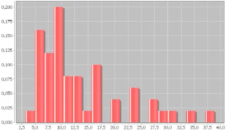
Two tests are performed to characterise the geometric accuracy of linear objects from OSM data: roads and coastline. For the road network, a selection of 50 pairs of homologous linear objects in the region of Hendaye is used.

Figure 7. Distribution of Hausdorff distances from the sample of roads

The distribution of Hausdorff distances shown in Figure 7 indicates a concentration between 5 and 15 meters with a peak between 5 and 10 meters. The average of maximum deviations (Table 2) reaches 13.57 meters. It is important to nuance the interpretation of extreme values (beyond 20 meters), which may be biased by the introduction of extremities of polylines (departure and arrival nodes) in the computation of Hausdorff distance. Once again, the standard deviation shows a significant heterogeneity in positional accuracy.

Table 2. Statistics calculated on distances between road linear features.

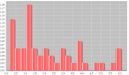
Distribution of average distances as shown in Figure 8 and Table 2 is fairly spread, but in very small distances (0 to 6 meters), knowing that in the reality, a road is around 6 meters

wide. The distances computed between OSM and BD TOPO® road networks are close to reference accuracy but the standard deviation nearly as important as the mean shows heterogeneity.

Figure 8. Distribution of average distances from the sample of roads

A comparison of the theme coastline is also conducted in the region of Hendaye, after

extraction of three pairs of homologous linear objects, as shown in Figure 9. Some portions of the coastline, with important differences, have not been taken into account. Indeed, the

coastline specified by IGN on the BD TOPO® (level of highest tides with a 120 tide coefficient) can penetrate deeply inlands in some estuaries. This area however may not be represented in OSM data, because of the lack of specifications of capture, and the subjectivity of the operator in his perception of the coastline.

Figure 9. Representation of the 3 sample couples of coastlines. The grey area shows the gap between each couple.

The couple No. 1 (Figure 9), captured in urban areas, present small differences (Hausdorff distance of 25.93 meters and average distance of 0.82 meters). Couples No. 2 and No. 3 (Figure 9), captured in areas of bays and cliffs, present significant differences, respectively Hausdorff distances of 139.66 meters and 154.56 meters, and average distances of 32.21 and 26.58 meters. The curvilinear abscise difference between the two couple’s reaches 11% of the total length of the reference dataset (BD TOPO®).

Such results are particularly interesting because they illustrate the importance of defining precise specifications to avoid subjectivity: subjectivity leads to big quality problems that could be easily avoided with specifications defining precisely what should be captured as a coastline and how it should be done.

1

3.3.3. Polygonal primitives

To characterise differences between polygonal objects, the distance used is the surface distance, proposed by Vauglin (1997) (Figure 10).

The distance is therefore surface dS: dS = 1 -









Figure 10. Surface distance between two polygons.

The surface distance is defined in the interval [0, 1]. If the distance is equal to 0, the two polygons are equal, if the distance is equal to 1, the two polygons are disjoint.

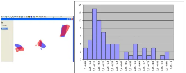
The comparison of polygonal objects is carried on the theme lakes in the mountainous region of l’Alpe d'Huez. A sample of 68 pairs of homologous surfaces is used (Figure 11).

Figure 11. Selection of OSM polygonal objects (blue) and BD Topo (red) and distribution of surface distances.

The distribution of surface distances (Figure 11) shows a concentration peak between 0.1 and 0.25, which corresponds to quite low differences.Indeed, Bel Hadj Ali and Vauglin (1999) proposed a polygon object matching process partly based on surface distance and considered such distribution as showing little difference. They compared cadastral buildings with

buildings from topographic data (considered as quite close in position and shape) and noticed that 25% were under 0.05, which is not the case here, and 70% were between 0.15 and 0.45.

0 2 4 6 8 10 12 14 0 0 ,0 5 0 ,0 5 0 ,1 0 ,1 0 ,1 5 0 ,1 5 0 ,2 0 ,2 0 ,2 5 0 ,2 5 0 ,3 0 ,3 0 ,3 5 0 ,3 5 0 ,4 0 ,4 0 ,4 5 0 ,4 5 0 ,5 0 ,5 0 ,5 5 0 ,5 5 0 ,6 0 ,6 0 ,6 5 0 ,6 5 0 ,7 0 ,7 0 ,7 5 0 ,7 5 0 ,8 0 ,8 0 ,8 5 0 ,8 5 0 ,9 0 ,9 0 ,9 5 0 ,9 5 1

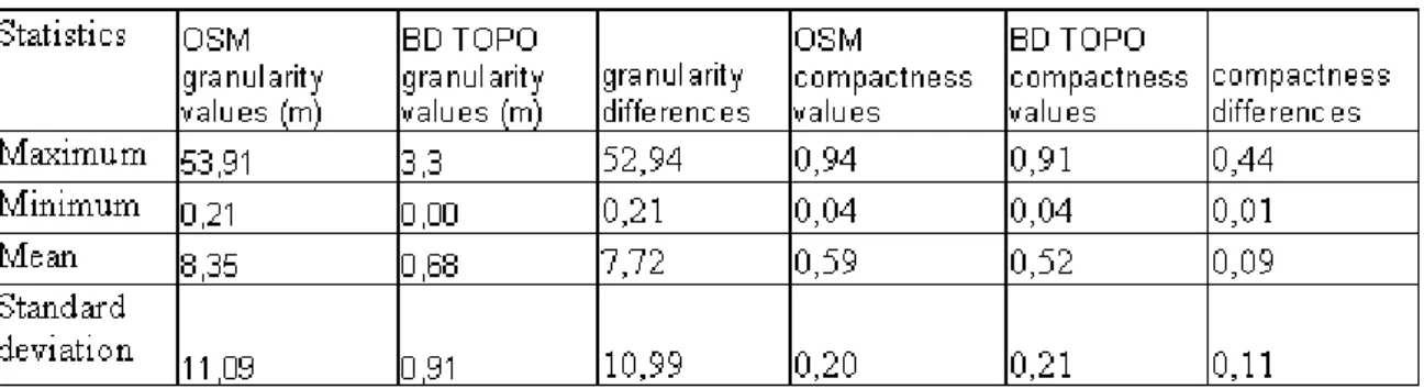
Table 3. Granularity and compactness statistical analysis of lakes in OSM and BD TOPO®.

However, comparison of polygonal primitives requires both a comparison of positions but also of shapes. To cope with this requirement, granularity and compactness measures were carried out on the same dataset (Table 3). The granularity measure used simply returns the shortest segment of the polygon. It measures resolution differences and the standard deviation shows great heterogeneity compared to BD TOPO®. Compactness is computed using Miller's measure (McEachren, 1985): 2 2 perimeter area C  

Compactness differences allow the assessment of shape differences between OSM lakes and BD TOPO ones. Table 3 show that, here, the differences are small.

3.4. Semantic and attribute accuracy

Table 4 shows quantitative results on attribute accuracy while Figure 12 shows qualitative assessment on attribute accuracy. Quantitative results show that the main tag of each type of objects analysed is mostly informed (except for roads where the ratio is only 85%) while the secondary attributes are rarely informed. Qualitative results are based on the same method as for geometry but using here the Levenstein distance that compares strings. Qualitative results show that only 55% of the lake names are informed as in BD TOPO® but when they are, the names are nearly identical (a distance of between 1 and 3 generally correspond to simple spelling mistakes).

Table 4. Quantitative attribute quality assessment: attribute filling of the shapefile layers extracted from CloudMade (October 2009) covering completely France.

Semantic accuracy assessment was also carried out on the nature or function of 585 roads represented in the tag highway in OSM data that was compared to the nature attribute of BD TOPO® roads. The main roads, corresponding to "Motorway" and "Primary" values have semantically correct classification as nearly 100% have their BD TOPO® homologous classified the same way. But only 49% of the secondary roads are semantically correct compared to BD TOPO®. The error made by the contributors is mainly the underestimation of road importance: roads considered as "secondary" in BD TOPO® are classified as

"Residential" or "Tertiary" in OSM data. The number of local roads in the OSM sample was to low to do the same comparison. Our interpretation is that when semantic classification specifications are clear like for main roads, the semantic accuracy is good which pleads once again for better specifications.

Figure 12. Statistics of Levenstein distance between lake names in OSM and BD TOPO® and distribution of the distances on the right.

Other qualitative remarks can be made on the heterogeneity of attribute values allowed in OSM. The One Way tag, when filled, contains in the whole French road data the values 0, 1, -1, yes, no, true or false.

Semantic and attribute accuracy are not guaranteed by the specifications which explains the quantitative and qualitative results. Several issues explain the low accuracy:

- Specifications, by their global reach, are extremely detailed but don’t cover a classification commonly accepted by all contributors, who according to their profiles will be concerned in a limited part of the semantic possibilities. This causes semantic incoherencies depending on contributors: for example, secondary, tertiary and residential roads will not be classified in the same way.

- Even if it is not recommended, you can enter tags and values that are not present in the specifications.

- There is not a commission for the management of names, no more than recommendations for formatting (capitalisation, prefixes, etc. ...). There is therefore a very high unaccuracy in the names that are captured in the tag "name": for example on the same point of interest, we can have "Eglise Saint Jacques" and "Ecole Saint-Jacques".

As a consequence, standardised specifications are highly required to improve semantic and attribute quality of OSM data.

0 5 10 15 20 25 30 35 0 2 2 4 4 6 6 8 8 1 0 1 0 1 2 1 2 1 4 1 4 1 6 1 6 1 8 1 8 2 0

3.5. Completeness

Figure 13. Heterogeneity of “Administrative Limit” layer completeness

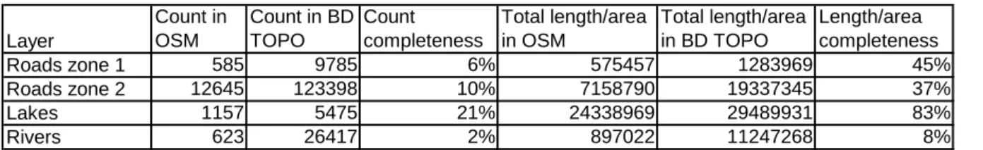
Goodchild (2009) claims that completeness and currentness are the most significant aspects of VGI quality. Some aspects of completeness are measured in Table 5. Regarding the number of objects, OSM is far from being complete for every theme considered. Regarding the total length/area of objects, the difference is less important. This result means that smaller objects are more likely to be absent, reflecting the fact that contributors are more focused on

capturing attracting objects (the most useful for their interest).

Table 5. Completeness analysis for different object layers with the BD TOPO® as reference.

It appears that the data density does not depend only on the density of information on the territory but also on the density of OSM contributors, that clearly excludes a number of territories (Figure 13). Thus, territories are best represented in rich areas and / or with a young population as shown by the extracts of the 15th arrondissement of Paris (Figure 14a) or the University Paul Sabatier in Toulouse (Figure 14b). The middle-size towns remain captured exhaustively, but lacks are observed at street level in some areas (Figure 15a). Completeness becomes very problematic in more rural and non profitable areas as in the Creuse (Figure 15a) where only a public utility mission would require surveys. Even in tourist areas like the Côte d'Azur, there are empty areas. Our assessment is confirmed by a more systematic analysis performed on English OSM data from Haklay (2009), who has shown that disadvantaged areas were less well covered.

Layer Count in OSM Count in BD TOPO Count completeness Total length/area in OSM Total length/area in BD TOPO Length/area completeness Roads zone 1 585 9785 6% 575457 1283969 45% Roads zone 2 12645 123398 10% 7158790 19337345 37% Lakes 1157 5475 21% 24338969 29489931 83% Rivers 623 26417 2% 897022 11247268 8%

Figure 14. Extracts of OSM in areas well covered where data is quite diverse and complete: (a) in the 15th arrondissement of Paris (b) on the University Paul Sabatier in Toulouse.

Figure 15. Extracts of OSM: (a) the town-center of Pau : medium-sized cities are moderately complete: most buildings and some streets are missing. (b) in Creuse: The information is extremely poor (municipal limits and some main roads).

3.6. Logical consistency

The logical consistency measures the consistency of different database objects with other objects of the same theme (intra-theme consistency) or objects of other themes (inter-theme consistency). For example, linear roads must be captured in network and must share the same geometry as the administrative boundaries when it is the case in the reality. Respect for logical consistency is generally done by the introduction of integrity constraints (Servigne et al, 2000). However, OSM does not contain any integrity constraints. Respect for logical consistency depends on the carefulness of each contributor during the capture. This results in a very bad logical consistency. Different cases of logical inconsistency of OSM data are presented below.

Figure 16. Problems of internal consistency in the road network: (a) roads are not connected at an intersection, (b) unstructured road network.

Regarding intra-theme consistency, connectivity of roads is relatively assured (approx. 95%) using the snapping capacity of the capture tools (Figure 16a) while in the BD TOPO ®, this

(a)

(b)

error is guaranteed at less than 1% using auto-correction tools. Furthermore the structure of the network is not at all guaranteed (Figure 16b) while a good model implicates to finish each line at every intersection (Egenhofer, 1993). Nevertheless, whatever the region tried, the use of a simple geoprocess in ArcGIS, that computes the administrative units from the linear limits, crashes because of bad topology. In this case, the bad intra-theme consistency limits the use of data like in the case of multiple captures of the same real world entity (Figure 17b).

Figure 17. (a) The selected administrative limit (blue) is not at all consistent with the roads (b) Several lakes are captured in the same location.

Regarding inter-theme consistency, Figure 17a and Figure 18 shows how the capture of the administrative boundary has been carried out independently of the roads or the coastline, which generates strong inconsistencies. Moreover some statistics have been computed on river/administrative limit consistency: 68% of the tested administrative unit are not consistent with rivers but with great heterogeneity. Some parts are completely consistent ("La Garonne" for example) but most are completely inconsistent ("La Seine").

Figure 18. Example of both types of inconsistencies: between administrative borders, that are sometimes captured on the coastline and sometimes not, and between coastline and administrative borders that should share geometry.

3.7. Currentness

The process of publication and diffusion of a particular update is faster in OSM, where contributions are automatically integrated without moderation. But the management of updates is not systematic and depends on the interests of contributors. Table 6 shows the evolution of French OSM data in number of objects over three months: a 30% mean increase for all objects. This evolution illustrates the reactivity of OSM contributors although the evolutions are mainly completions than updates.

Table 6. Comparison of “France_shapefile” themes (extracted from CloudMade) between June 2009 and October 2009.

3.8. Lineage

A data lineage is provided: a comment about the data storage is associated to the contributor. However, we don’t know how the data were captured except the software used. We do not know which support was used, as GPS tracks or satellite imagery. This can be quite annoying in the case of data for which methods can be multiple or even illegal. Instead, in the BD TOPO ®, a source attribute informs the method used to capture data (photo restitution, map or field collection...).

Moreover, the historic of modifications is not kept, making the integration of institutional data difficult: if the geometry is changed, it becomes impossible to propagate the official updates. Goodchild (2008) claims that each contributor cannot be trusted the same between institutions qualified as authoritative and simple contributors that are at most asserted. Coleman et al (2009) confirms such confidence differences and proposes call upon moderators like in Wikipedia to control the different type of contributions. A proper lineage metadata would allow to grant trustful contributions with rights forbidding less trustful contributions to update them.

3.9. Usage

Following the precedent discussion, we agree with the conclusions of Haklay (2009) that typical applications of OSM vector data appear to be limited to mapping. Navigation

applications are limited by the problems of logical consistency: it is necessary to restructure all data in a GIS to use them for navigation, but then the lack of completeness would cause errors hardly acceptable. Road and river topological inconsistencies would also prevent the network be automatically pruned (Touya, 2007) which is necessary to display it at different scales. Even classical geo-processing process like generating administrative polygons from limits massively fails because of low quality logical consistency (see section 3.6). Urban planning applications would be limited in particular by the strong heterogeneity of geometric precision. Finally, any application based on OSM data would face major problems of updating management.

The strong heterogeneity of OSM data resolution also affects their mapping. Ruas (2004) shows that resolution and scale represent key concepts in cartographic visualisation linked to generalisation purposes (Mackaness et al, 2007). Differences in resolution between themes, or with other themes, severely limit the possibility of automatic generalisation, and therefore, a correct representation of data at different scales. This also blocks a real definition of the

Layer Objects – june 09 Objects – oct 09 Evolution (objects) Evolution (%) France_poi 76653 111440 34787 45,4% France_highway 674205 886680 212475 31,5% France_coastline 1201 1200 -1 0% France_administrative 42286 51413 9127 21,5% France_water 10531 12507 1976 18,8% France_natural 20958 24756 3798 18,1% TOTAL 825834 1087996 262162 31,7%

reference scale of these data, which corresponds in the optimal scale for mapping (Mackaness et al, 2007).

4. Specifications to Improve VGI Quality

The evaluation of different aspects of OSM data quality reveal the key role of specifications to ensure quality as several error types come from a lack or fuzzy specifications. The

specifications of a geographic database gather the selection and modelling choices of the database (Figure 19). In OSM, the specifications are rich and complex but informal specifications instead of being recorded in written formalised and well accepted

specifications. A contributor is advised to follow the specification but does not have to. For instance, the inaccuracy of the coastline (Figure 9) is due to a lack of capture specifications: expert contributors aware of the challenges of quality and consistent contributions will strictly meet the specifications while novice contributors will probably ignore them. Goodchild (2008) agrees with the idea that VGI data lack standardised and precise specifications to be quality geographic data. Indeed, he claims that although crowdsourcing has proved qualitative in different domains, geographic information has particularities that require modelling and capture agreements.

Figure 19. Production process of structured institutional databases (Balley et al, 2006).

Gesbert (2005) proposes a formal model for geographic database specifications to allow the specifications to be machine-interpretable. Abadie (2009) extends this formalisation to propose an XML specification model that helps to detect automatically inconsistencies in data, which could be useful to improve OSM data.

The definition of a reference scale and of a resolution (Ruas, 2004) is also related to the definition of specifications. The capture of a contribution should be based on a reference scale, a resolution described in the specifications to avoid resolution heterogeneity.

OpenStreetMaps clearly lacks reference scale ranges: captured data should be specified to be used in a specific scale range where its quality and resolution is good enough like in the

Real World Categorisation Selection

Modelling

Implementation Capture

A real world lake: permanent water area …

Lakes with area > 50 m² are represented

…

A lake will be a surfacic object with name and identifier attributes

… Logical data model

Which real world objects are observed?

For each type, which objects are represented?

Which conceptual data model to represent the objects?

Which logical data model to implement the objects?

ScaleMaster (Brewer and Buttenfield, 2007). Actually, each OSM feature has its own reference scale and resolution (buildings and built-up areas do not have the same resolution but coexist in OSM) but the information is not available in metadata.

However, Coleman et al (2009) show that the majority of VGI contributors are occasional contributors and mostly interested amateurs that could be afraid of strict specifications for contributions. The success of VGI lies in the simplicity of contributions and many debates in the OSM contributor community show that should not be too restrained, even to improve quality. We believe that the improvement of OSM data quality requires to find the ideal balance between specifications and contribution freedom. A convenient way to reach such balance is to use automatic consistency checking with strict specification. Brando and Bucher (2010) propose to let contributions be simple and free but to check contribution consistency with the specifications. The automatic process would provide corrected and consistent contribution to the contributor that would be free to accept the modifications or not.

6. Conclusion and further work

In conclusion, this article assessed the data quality of the reference site for free and contributively created data OpenStreetMap. We described its models and objectives and assessed its data quality by comparing different components with an IGN database as a reference. We have shown that a production model of topographic data such as OSM has the advantage of responsiveness, flexibility, enabling a wealth of contents in privileged places. But the main drawback is a very high heterogeneity in several domains, limiting highly the possible applications. The contribution of the paper is the demonstration that data quality should not be summarised to geometrical position. The heterogeneity is due to the lack of standardised and precise specifications to would allow contributors to provide good quality data.

In perspective, improvements and evolution of quality control processes represent an integrant part of ongoing researches in the conception of an evaluation model of geometric imprecision in under qualified vector databases using, or not, reference datasets. The aim of this work is also to produce a more relevant and useful information on spatial data quality to the final user, based on knowledge of processes of production. Those first experimentations performed on OSM databases can help to calibrate the future model and also propose a first reference in the evaluation of OSM data quality, with Haklay (2009). A final issue that will be tackled is the use of formal specifications to allow good quality VGI: a PhD has just started in our lab on this specific topic.

Acknowledgments

We first thank Damien Boilley, an OpenStreetMap passionate contributor for his explanations on the project. We also thank Bénédicte Bucher, who initiated this study.

References

Abadie N 2009 Formal specifications to automatically identify heterogeneities. Proceedings of 12th International Conference

on Geographic Information Science (AGILE'09), Pre-Conference Workshop “Challenges in Spatial Data

Harmonisation”, Hannover (Germany).

Allan A 2008 Osm cycle maps. In Proceedings of 44th Annual Summer School. Society of Cartographers, 2008.

Balley S, Bucher B, Libourel T 2006 A service to customize the structure of a geographical dataset. In Proceedings of

Semantic Based GIS workshop (SEBGIS), Montpellier, France.

Bel Hadj Ali A, Vauglin F 1999 Geometrical Matching of Polygons in GISs and Assessment of Geometrical Quality of Polygons. In Proceedings of the International Symposium on Spatial Data Quality (ISSDQ'99), Hong Kong: 33-41 Brewer C, Buttenfield B 2007 Framing Guidelines for Multi-Scale Map Design Using Databases at Multiple Resolutions.

Cartography and Geographic Information Science 34 (1): 3-15.

Bucher B, Brasebin M, Buard E, Grosso E, Mustière S 2009 GeOxygene: built on top of the expertness of the French NMA to host and share advanced GI Science research results. In Proceedings of International Opensource Geospatial Research

Symposium 2009 (OGRS'09), 8-10 July, Nantes (France).

Coleman D J, Georgiadou Y, Labonte J 2009 Volunteered Geographic Information: the nature of motivation of produsers.

International Journal of Spatial Data Infrastructures Research 4, Special Issue GSDI-11.

Egenhofer M 1993 What's Special about Spatial, Database Requirements for Vehicle Navigation in Geographic Space.

SIGMOD Record 22, n°2, Washington D.C., 1993: 398-402

Gesbert N 2004 Formalisation of Geographical Database Specifications. Proceedings of 8th conference on Advanced

Databases and Information Systems (ADBIS'04), 22-25 September, Budapest (Hungary)

Goodchild M F 1992 Geographical data modelling. Computers & Geosciences 18, n°4: 401-408.

Goodchild M F 2007 Citizens as Voluntary Sensors: Spatial Data Infrastructure in the World of Web 2.0. International

Journal of Spatial Data Infrastructures Research 2: 24-32.

Goodchild M F 2008 Spatial Accuracy 2.0. In Proceedings of the 8th _{International Symposium on Spatial Data Accuracy}

Assessment in Natural Resources and Environmental Sciences, Shangai, China: 1-7.

Goodwin J, Dolbear C, Hart J 2008 Geographical Linked Data: The Administrative Geography of Great Britain on the Semantic Web. Transactions in GIS 12, 1: 19-30

Haklay M 2009 How good is OpenStreetMap information? A comparative study of OpenStreetMap and Ordnance Survey datasets for London and the rest of England. Environment & Planning B, to be published.

Jackobsson A, Vauglin F 2001 Status of Data Quality in European National Mapping Agencies. In Proceedings of 20th

International Cartographic Conference, ICA, Beijing, China 2001, vol 5: 2875-2883.

Kresse W, Fadaie K 2003 Iso Standards for Geographic Information. Springer-Verlag Berlin and Heidelberg GmbH & Co. K, 2003.

Lemmens R 2006 Semantic Interoperability of Distributed Geo-Services ". PhD thesis, ITC, Netherlands.

MacEachren A M 1985 Compactness of geographic shape: comparison and evaluation of measures. Geografiska Annaler

67(B): 53-67

Mackaness W, Ruas A, Sarjakoski T 2007 Generalisation of geographic information: cartographic modelling and applications. Elsevier.

Manola F, Miller E 2004 RDF Primer, W3C Recommendation. WWW document,

http://www.w3.org/TR/rdf-primer/.

McMaster R 1986 A statistical Analysis of Mathematical Measures for Linear Simplification. The American Cartographer

23, 1986.

Perret J, Boffet Mas A, Ruas A 2009 Understanding Urban Dynamics : the use of vector topographic databases and the

creation of spatio-temporal databases. In Proceedings of 24th _{International Cartographic Conference, ICA, Santiago}

(Chile), 15-21 november 2009.

Ruas A 2004 Le changement de niveau de détail dans la représentation de l'information géographique. Habilitation thesis, Université Marne la Vallée.

Servigne S, Ubeda T, Puricelli A, Laurini R 2000 A Methodology for Spatial Consistency Improvement of Geographic Databases. GeoInformatica 4, n°1, 2000: 7-34

Sui D Z 2008 The wikification of GIS and its consequences: Or Angelina Jolie's new tattoo and the future of GIS ".

Computers, Environment and Urban Systems 32, n°1: 1-5.

Tapscott D, Williams A D 2007 Wikinomics: How Mass Collaboration Changes Everything. Hardcover, 2007. Touya G 2004 Elaboration d’un fond cartographique départemental. Master Thesis, ENSG.

Touya G 2007 River Network Generalisation based on Structure and Pattern Recognition. In Proceedings of 23rd

International Cartographic Conference, ICA, Moscow (Russia).

Vauglin F 1997 Modèles statistiques des imprécisions géométriques des objets géographiques linéaires. PhD Thesis, Université Marne la Vallée.