HAL Id: inserm-00502110
https://www.hal.inserm.fr/inserm-00502110
Submitted on 18 Feb 2011
HAL is a multi-disciplinary open access
archive for the deposit and dissemination of
sci-entific research documents, whether they are
pub-lished or not. The documents may come from
teaching and research institutions in France or
abroad, or from public or private research centers.
L’archive ouverte pluridisciplinaire HAL, est
destinée au dépôt et à la diffusion de documents
scientifiques de niveau recherche, publiés ou non,
émanant des établissements d’enseignement et de
recherche français ou étrangers, des laboratoires
publics ou privés.
Jiasong Wu, Huazhong Shu, Lu Wang, Lotfi Senhadji
To cite this version:
Jiasong Wu, Huazhong Shu, Lu Wang, Lotfi Senhadji. Fast algorithms for the computation of sliding
sequency-ordered complex Hadamard transform. IEEE Transactions on Signal Processing, Institute
of Electrical and Electronics Engineers, 2010, 58 (11), pp.5901-5909. �10.1109/TSP.2010.2063026�.
�inserm-00502110�
Abstract—Fast algorithms for computing the forward and
inverse sequency-ordered complex Hadamard transforms (SCHT) in a sliding window are presented. The first algorithm consists of decomposing a length-N inverse SCHT (ISCHT) into two length-N/2 ISCHTs. The second algorithm, calculating the values of window i+N/4 from those of window i and one length-N/4 ISCHT and one length-N/4 modified ISCHT (MISCHT), is implemented by two schemes to achieve a good compromise between the computation complexity and the implementation complexity. The forward SCHT algorithm can be obtained by transposing the signal flow graph of the ISCHT. The proposed algorithms require O(N) arithmetic operations and thus are more efficient than the block-based algorithms as well as those based on the sliding FFT or the sliding DFT. The application of the sliding ISCHT in transform domain adaptive filtering (TDAF) is also discussed with supporting simulation results.
Index Terms—Fast algorithm, sequency-ordered complex
Hadamard transform, sliding algorithm
I. INTRODUCTION
HE discrete orthogonal transforms play an important role in the fields of digital signal processing, filtering and communications. In the past decades, various transforms including discrete Fourier transform (DFT) [1], discrete Hartley transform (DHT) [2], discrete cosine transform (DCT) and discrete sine transform (DST) [3], and Walsh-Hadamard
This work was supported by the National Natural Science Foundation of China under Grant 60873048, by the National Basic Research Program of China under Grant 2010CB732503, by a Program of Jiangsu Province under Grant SBK200910055 and the Natural Science Foundation of Jiangsu Province under Grant BK2008279. This work is also supported by the “Eiffel Doctorate” excellence grant of the French Ministry of Foreign and European Affairs.
J. Wu is with the Laboratory of Image Science and Technology, School of Biological Science and Medical Engineering, Southeast University, Nanjing 210096, China, the Centre de Recherche en Information Biomédicale Sino-Français (CRIBs), Nanjing 210096, China, INSERM, U 642, 35000 Rennes, France, and the Laboratoire Traitement du Signal et de l’Image (LTSI), Université de Rennes 1, 35000 Rennes, France (e-mail: [email protected]).
H. Shu and L. Wang are with the Laboratory of Image Science and Technology, School of Computer Science and Engineering, Southeast University, Nanjing 210096, China, and also with the Centre de Recherche en Information Biomédicale Sino-Français (CRIBs), Nanjing 210096, China (e-mail: shu. [email protected]; [email protected]).
L. Senhadji is with INSERM, U 642, 35000 Rennes, France, with the Laboratoire Traitement du Signal et de l’Image (LTSI), Université de Rennes 1, 35000 Rennes, France, and with the Centre de Recherche en Information Biomédicale Sino–Français (CRIBs), 35000 Rennes, France (e-mail: [email protected]).
transform (WHT) [4], [5] have been introduced and found wide applications in many scientific and technological areas. Recently, Aung et al. introduced the sequency-ordered complex Hadamard transform (SCHT) [6], which can be an alternative of DFT in some applications requiring lower computational complexity such as spectrum analysis and image watermarking. It was shown that the SCHT performs better than the WHT in asynchronous CDMA system [7]. Two
block-based algorithms including the radix-2
decimation-in-time (DIT) [6] and decimation-in-sequency (DIS) [8] have been developed for fast computation of SCHT.
An interesting case appears when the spectrum of a nonstationary process, such as speech, radar, biomedical, and communication signals, is required. This leads to the so-called sliding transform, also known as time-dependent or short-time transform [1], to determine the time-varying spectrum. Basically, the sliding transform means that the transform is computed on a fixed-length window of the signal, which is continuously updated with new samples as the oldest ones are discarded [9]. In such cases, the signal properties (amplitudes, frequencies, and phases) usually change with time, a single orthogonal transform is not sufficient to describe the entire signal [10], [11]. Assume that the window contains N complex values xi, xi+1, …, xi+N–1 at time instant i, then, the sliding
orthogonal transform is defined by [10]
, (1)
where wm is a window function, and is an
orthogonal basis set. YN(k, i) represent the orthogonal
transform of the windowed signal around time i.
In the past, the sliding orthogonal transforms have been investigated and found applications in spectrogram analysis and adaptive filter design. Since the computation of sliding transform at each position of a sliding window is an intensive task, many fast algorithms were proposed [9-24]. Among them, the sliding FFT [14-16] and the sliding DFT [17-19] have attracted many attentions due to their extensive applications. By applying a property of radix-2 DIT FFT algorithm, Farhang-Boroujeny et al. proposed an efficient sliding FFT algorithm, which needs 4N–8log2N real
multiplications, log2N–1 multiplications with the imaginary
number j and 4N–4log2N–2 real additions [14], [15]. The
sliding FFT algorithm was then extended to other discrete orthogonal transforms such as DHT, DCT, DST and WHT [16]. Based on the circular shift property of DFT, Jacobsen and Lyons developed a fast sliding DFT algorithm, which
Fast algorithms for the computation of sliding
sequency-ordered complex Hadamard transform
Jiasong Wu, Member, IEEE, Huazhong Shu, Senior Member, IEEE, Lu Wang and Lotfi Senhadji,
Senior Member, IEEE
Recently, special attention has also been paid on the fast computation of sliding WHT [20-24] due to the real-time application requirement of pattern matching in many cases, such as video block motion estimation in H. 264 [21]. A fast algorithm, based on the radix-2 DIS WHT algorithm, which decomposes a length-N WHT into two length-N/2 WHTs plus 2N–2 additions, for the sliding WHT was proposed in [22]. This algorithm was further improved by Ben-Artzi et al. [23], who proposed the gray code kernel algorithm that utilizes the previously computed values in the leaves of the tree structure. Ouyang and Cham [24] presented a more efficient algorithm to compute the sliding WHT, which computes the length-N WHT from two length-N/4 WHTs plus 3N/2+1 additions.
Inspired by the research work presented in [22] and [24], we propose in this correspondence two fast algorithms for efficient computation of sliding SCHTs. The first algorithm consists of decomposing a length-N inverse SCHT (ISCHT) into two length-N/2 ISCHTs. The second algorithm, calculating the values of window i+N/4 from those of window
i and one length-N/4 ISCHT and one length-N/4 Modified
ISCHT (MISCHT), is implemented by two schemes to achieve a good compromise between the computation complexity and the implementation complexity.
The paper is organized as follows. In Section II, preliminaries about the forward and inverse sliding SCHTs are given. The proposed sliding ISCHT algorithms are described and the comparison results with other algorithms are provided in Section III. Transform domain adaptive filtering is given in Section IV to illustrate the potential application of sliding ISCHT. Section V concludes the paper.
II.
P
RELIMINARYIn this section, we first give the definition of sliding SCHT based on the general sliding transform given in (1) and SCHT in [6]. Consider M input signal elements xi where i = 0, 1, …,
M–1, which is divided into overlapping windows of size N (M
> N). Let XN(i) = [xi, xi+1, …, xi+N–1]T and YN(i) = [yi, yi+1, …,
yi+N–1]T be respectively the complex input vector and the
transformed complex vector of the ith window, where T denotes the transposition, and let N = 2n, n ≥ 1, the length-N
forward and inverse sliding SCHTs are defined as [6]
(2)
(3)
where the superscript H denotes the Hermitian transposition,
HN is the order-N ISCHT matrix whose elements are given by
(4) where (5) (6) (8) From (4) to (8), we have (9)
If we ignore the normalization factor 1/N in (2), it can be seen that the implementation of the forward sliding SCHT can be obtained by transposing the signal flow graph of the sliding ISCHT. Therefore, for simplicity, we take the sliding ISCHT into consideration. Let
(10)
(11)
where HN(k), k = 0, 1, …, N–1, is the kth column of ISCHT
matrix . , k = 0, 1, …, N–1, is the kth row of . Note that the matrix verifies the symmetry
property, that is, .
Let xN(k, i) be the kth ISCHT projection value for the ith
window, that is
for k = 0, 1, …N–1; i = 0, 1, …, M–N, (12) Let us also define
for k=1, 3, …, N–1; i = 0, 1, …, M–N; N = 2n, n ≥ 2.
(13)
Equation (3) can then be rewritten as
III. FAST ALGORITHMS FOR SLIDING ISCHT
In this section, we derive two fast algorithms for computing the sliding ISCHT.
Algorithm 1: Decomposing a length-N ISCHT into two length-N/2 ISCHTs
By performing a similar strategy as presented in [22], and by utilizing a property of radix-2 DIS ISCHT algorithm, we extend the algorithm proposed in [8] to the sliding ISCHT algorithm. By performing the radix-2 DIS method on HN [8],
we have
(15)
where IN is the identity matrix of order N,
(16) and PN is the permutation matrix such that for the input vector YN(i):
(17) Equation (15) can be rewritten as
(18)
(19)
where is the Kronecker product and denotes the lower integer part of x. The starting point is
.
The tree structure of ISCHT matrix construction is shown in Fig. 1. Using the projection relationships in (12) and (13), (18) and (19) can be equivalently expressed as their projection values:
(20)
(21)
The starting point is . So far, the algorithm in [8] has been extended to the
sliding ISCHT. The main difference between (18) and (20) is that the latter computes the current projection values from those of the last layer in the tree structure shown in Fig. 1. Using a similar analysis of the computational complexity and
memory storage requirement reported in [14-16] and [22], it can be seen that N/2–1 multiplications with j, 2(N–1) complex additions, and 2N(log2N–1) words of memory are needed for
computing the length-N = 2n sliding ISCHT. Note that the
multiplication by j or –j can be realized by switching the real and imaginary parts of the input with one sign changing, so that there is no memory storage requirement. As stated in [8], the operations of swapping and subtraction can be jointly performed with the help of the 2:1 complex multiplexers to accomplish the multiplications with –j. The proposed
Algorithm 1 is similar to the algorithm reported in [22], but
slightly different from the sliding FFT algorithms [14-16] since the latter are based on the radix-2 DIT FFT algorithm. Note that if we extend the radix-2 DIT ISCHT algorithm [6] to sliding algorithm, we obtain exactly the same algorithm as those presented in [14-16].
Algorithm 2: Computing the values of window i+N/4 from those of window i and one length-N/4 ISCHT and one length-N/4 MISCHT
Inspired by a research work presented in [24], we propose another algorithm which computes the values of length-N sliding ISCHT of window i+N/4 from those of window i.
A. Fast algorithm for N = 4
The proposed algorithm is shown in Table I, from which we have (22) where (23) (24)
B. Fast algorithm for N = 8
The proposed algorithm is shown in Table II, from which we have (25) where (26) (27)
where S2 and P4 are respectively defined in (16) and (17).
C. Fast algorithm for N = 2n, n ≥ 3
Using the same strategy as for N = 4 and N = 8, we have (28)
(29)
, (30)
where SN and PN are given in (16) and (17).
The derivation of (28) is given in Appendix. Fig. 2 shows the signal graph of the proposed Algorithm 2, whose computational complexity and memory storage requirement are analyzed as follows (assuming that the algorithm is implemented in parallel):
1) The computation of (30) for u = N/4–1 needs 1 complex addition. Note that the values of dN(i+u), u = 0, 1, …, N/4–2,
have already been obtained during the computation of xN(k,
i+v), v = 1, 2, …, N/4–1. Memory size of N/2 is required for
storing dN(i+u), u = 0, 1, …, N/4–1. The input yi+u and yi+N+u
for u = 0, 1, …, N/4–1, needs N memory, which can be released after performing (30) since it will not be used in the following steps.
2) The computation of (29) needs a length-N/4 ISCHT (HN/4)
and a length-N/4 MISCHT (HN/4SN/4). Memory size of N is
needed for storing the values tN/2(i+u), u = 0, 1, …, N/2 – 1.
We also assume that the computation of length-N/4 ISCHT
and length-N/4 modified ISCHT needs and
memory, respectively.
3) The computation of (28) needs N/2 multiplications with j and N complex additions. The values of xN(k, i+v), v = 0, 1,
…, N/4–1, can be obtained by zero padding method reported in [21]. For the implementation, we first distribute 2N memory for xN(k, i), k = 0, 1, …, N–1, which is then overlaid
by xN(k, i+N/4), k = 0, 1, …, N–1 after performing (28).
Thus, the computational complexity and memory storage requirement of Algorithm 2 are given by
(31) (32) Note that the additions shown in (31) are complex additions.
In the following, we discuss the way to compute HN/4 and HN/4SN/4 appearing in (29). For the length-N/4 MISCHT
HN/4SN/4, the input data is first multiplied by SN/4, resulting in
the change of the two inputs: dN(i) replaced by jdN(i+N/4) and
jdN(i+N/8) by dN(i+N/8). This change makes the
implementation of HN/4SN/4 not exactly the same as that of HN/4. So algorithm 1 is used for the implementation of
HN/4SN/4. On the contrary, the length-N/4 ISCHT HN/4 can be
implemented by either algorithm 1 or algorithm 2. Therefore, two schemes are presented in the following.
In this case, (31) becomes
(33)
with the initial value and
The memory complexity in (32) becomes
(34)
with the initial values and .
Scheme 2: Implementing both length-N/4 ISCHT and MISCHT by algorithm 1
In this case, the computational complexity in (31) becomes
for N = 2m, m ≥ 4. (35)
From (32), the memory storage requirement is given by (36) It should be noted that the above algorithm can not be simply obtained from the existing sliding DFT and related algorithms. Generally speaking, the sliding DFT utilizes the first-order shift property [17-19] to establish the relationship between
xN(k, i+1) and xN(k, i), and other discrete orthogonal transforms
(DCT, DST, DHT) use the first-order shift property [12] or the second-order shift property [9-11] to establish the relationship between xN(k, i+1), xN(k, i) and xN(k, i-1). However, the
proposed Algorithm 2 establishes the relationship between xN(k,
i+N/4) and xN(k, i).
When using the algorithms in [6] and [8], N(log2N–1)/4
multiplications with j, Nlog2N complex additions and 2N
memory are needed for length-N ISCHT. The comparison results are shown in Table III. It can be seen from this table that the proposed algorithms reduce significantly the real additions compared to the algorithms reported in [6] and [8], but at the cost of a little more memory storage requirement. The computational complexity and the memory storage requirement of the sliding FFT in [14-16] and sliding DFT in [17-19] are shown in Table IV. For comparison purpose, Tables III and IV give the real multiplications, multiplications with j and real additions where one complex multiplication is implemented by four real multiplications and two real additions. Note also that when analyzing the complexity of the sliding FFT and the sliding DFT, the savings of the special
twiddle factors ( ) have been taken into account. As can be seen from Tables III and IV, the proposed algorithms are also more efficient than the algorithms shown in [14-19]. This is because the proposed algorithms only need the multiplications with j and real additions, and can save the memory for storing the twiddle factors.
The computation of the forward SCHT, if ignoring the normalization factor 1/N, can be simply realized by replacing j by –j in (16), HN by in (18)-(21) and x by y in (28)-(30).
IV. AN APPLICATIONEXAMPLE
In this section, we gave an example of ISCHT domain least-mean-square (LMS) adaptive filter with supporting simulation result to illustrate the potential application.
Transform domain LMS adaptive filters (TDLMSAF) introduced by Narayan et al.[25], exploit the de-correlation properties of some well-known signal transforms such as DFT, DCT, DHT and WHT, in order to pre-whiten the input data and speed up filter convergence [p413, 26]. For a given process x(n), the performance of the TDLMSAF algorithm may vary significantly depending on the selection of the transformation matrix T. A transform which performs well for a given input process may perform poorly once the statistics of the input change [p210-p211, 27].
Similar to the DFT domain LMS adaptive filter [25-28], the ISCHT domain LMS adaptive filter algorithm, shown in Fig. 3, is described as follows:
The input signal vector is first transformed into ISCHT domain by
(37) Then, is multiplied by the ISCHT domain adaptive weight vector
(38) to obtain the filter output
(39) The output error is given by
(40) where d(i) denotes the desired response.
The weight vector WN(i) is updated by the power-normalized
LMS algorithm
(41)
where µ is a positive step-size, e(i) is the output error and D(i) is a diagonal matrix of the estimated input powers which is defined by
(42) The aforementioned transform domain LMS adaptive filters with the proposed sliding ISCHT algorithms, sliding FFT [14-16] and sliding DFT [17-19] have been implemented using “C++” programming language. The execution time
comparison and signal-to-noise ratio (SNR) analysis between the proposed algorithms and sliding FFT and sliding DFT are carried out on a PC machine, which has an AMD single core CPU with speed of 3200MHz and 4096MB RAM. The run time of these algorithms have been calculated using GNU GCC complier version 3.4.5.
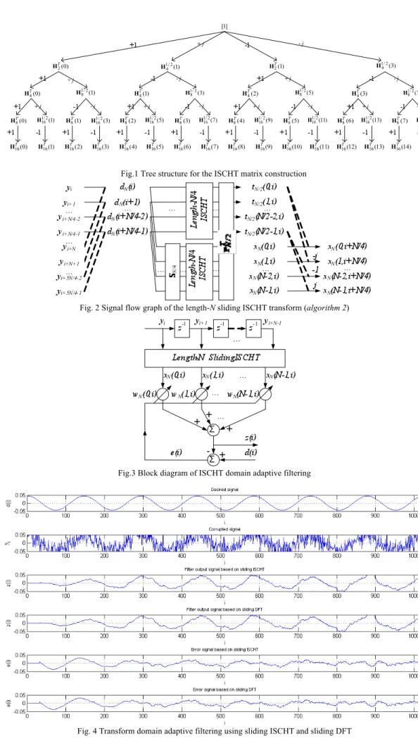
In this example, a 7 Hz sinusoid with 1024 samples per second corrupted by additive Gaussian white noise with SNR equal to 0dB is processed through the 32-tap filter. The parameters are set as µ = 0.01 and β = 0.9. The resulting SNRs of filtered signals by TDLMSAF using sliding ISCHT, sliding FFT, and sliding DFT are exactly the same (6.98dB). Fig. 4 shows the desired signal, corrupted signal and the filtered signals processed by TDLMSAF. Table V shows the execution time of sliding transforms and their corresponding TDLMSAFs. The execution times represent the average obtained by repeating the execution of the algorithms. It can be seen from this table that the proposed sliding ISCHT saves 10.0%-13.9% compared to sliding DFT, and saves 22.4%-25.8% compared to sliding FFT in the execution of sliding transformations. While the TDLMSAF with proposed sliding ISCHT is 3.3%-4.1% faster than TDLMSAF with sliding DFT, and 6.4%-7.3% faster than TDLMSAF with sliding FFT.
V. CONCLUSION
In this correspondence, we have presented two fast algorithms for computing the forward and inverse sliding SCHT. The arithmetic complexity order of the proposed algorithms is N, a factor of log2N improvement is made over
the block-based algorithm for the length-N SCHT. The proposed algorithms are also more efficient than that of the sliding FFT algorithm and the sliding DFT algorithm. The application of sliding ISCHT to transform domain adaptive filtering (TDAF) has been discussed. Note that the proposed algorithms can be easily extended to multidimensional case.
APPENDIX
To prove (28), we need first the following lemma:
Lemma 1: Let hN(k, l) be the (kth, lth) element of the
matrix HN, then we have
Proof: By the definition of hN(k, l) given in (4), we have
(A1) where (A2) Using (7), (6) becomes
On the other hand, it can be deduced from (8) that
(A4)
(A5)
Using (6), (A4) and (A3), we have
(A6)
Substituting (A6) into (A1) leads to
(A7)
The proof of can be
done in a similar way by using the relationship (A5). Lemma 2: The following relationship holds for k = 0, 1, …,
N/2 – 1, l = 0, 1, …, N/4 – 1
. (A8) Proof: Letting m = 2k, m and m+1 can then be expressed in binary representation as (A9) (A10) Thus (A11) (A12)
Since 0 ≤ l ≤ N/4–1, we have , it can be deduced
from (6) and (8) that
(A13)
The proof has been completed.
Based on the above two lemma, we provide the derivation of (28) in the following.
Equation (12) can be written as
(A14)
Similarly,
(A15) Using Lemma 1, (A14) and (A15) become
(A16)
(A17)
(A16) can be rewritten as
(A18) Substituting (A18) into (A17), we have
(A19) where , l = 0, 1, …, N/4–1, (A20) k = 0, 1, …, N–1. (A21)
From (18), we have
, k = 0, 1, …, N/2–1, l = 0, 1, …,
N/4–1. (A22)
Using Lemma 2 and (A22), we obtain
(A23) The above equation can be expressed in matrix representation as
(A24)
Using the relationship and (15), we
obtain
(A25) The proof of (28) has been completed.
ACKNOWLEDGMENT
The authors would like to thank the reviewers and Associate Editor Dr. Gross for their insightful suggestions for improving the manuscript. We are also thankful to Dr. Aung for providing his MATLAB code constructing the SCHT matrix and Dr. Ouyang for helpful discussion.
REFERENCES
[1] O.K. Ersoy, “A comparative review of real and complex Fourier-related transforms,” Proc. IEEE, vol. 82, pp. 429-447, 1994..
[2] N.C. Hu, H. I. Chang, and O. K. Ersoy, “Generalized discrete Hartley transforms,” IEEE Trans. Signal Process., vol. 40, no. 12, pp. 2931-2940, 1992.
[3] A.K. Jain, “A sinusoidal family of unitary transforms,” IEEE Trans.
Pattern Anal. Machine Intell., vol. 1, no. 10, pp. 356-365, 1979.
[4] S. Boussakta and A.G.J. Holt, “Fast algorithm for calculation of both Walsh-Hadamard and Fourier transforms (FWFTs),” Electron. Lett., vol. 25, no. 20, pp. 1352–1354, 1989.
[5] B. Arambepola and K. Partington, “Walsh-Hadamard transform for complex-valued signal,” Electron. Lett., vol. 28, no. 3, pp. 259-261, 1992.
[6] A. Aung, B.P. Ng, and S. Rahardja, “Sequency-ordered complex Hadamard transform: Properties, computational complexity and applications,” IEEE Trans. Signal Process., vol. 56, no. 8, pp. 3562–3571, Aug. 2008.
[7] A. Aung, B.P. Ng, and S. Rahardja, “Performance of SCHT sequences in asynchronous CDMA system,” IEEE Commun. Lett., vol. 11, pp. 641–643, 2007.
[8] G. Bi, A. Aung, and B.P. Ng, “Pipelined hardware structure for sequency-ordered complex Hadamard transform,” IEEE Signal Process.
Lett., vol. 15, pp. 401–404, 2008.
[9] J.A.R. Macias and A.G. Exposito, “Recursive formulation of short-time discrete trigonometric transforms,” IEEE Trans. Circuits.Syst. II, vol. 45, no. 4, pp. 525–527, Apr. 1998.
[10] V. Kober, “Fast algorithms for the computation of sliding discrete sinusoidal transforms,” IEEE Trans. Signal Process., vol. 52, no. 6, pp. 1704–1710, Jun. 2004.
[11] V. Kober, “Fast algorithms for the computation of sliding discrete Hartley transforms,” IEEE Trans. Signal Process., vol. 55, no. 6, pp. 2937–2944, Jun. 2007.
[12] J.-C. Liu and T.-P. Lin, “Running DHT and real-time DHT analyzer,”
Electron. Lett., vol. 24, no. 12, pp. 762–763, 1988.
[13] M. Jarmasz and G.A. Martens, “Simple design for a fast sliding DFT computer,” IEEE ICASSP’82. vol. 7, May 1982, pp. 502 – 505. [14] B. Farhang-Boroujeny and Y.C. Lim, “A comment on the computational
complexity of sliding FFT,” IEEE Trans. Circuits Syst., vol. 39, no. 12, pp. 875-876, Dec. 1992.
[15] B. Farhang-Boroujeny and S. Gazor, “Generalized sliding FFT and its application to implementation of block LMS adaptive filters,” IEEE
Trans. Signal Process., vol. 42, no. 3, pp. 532-538, Mar. 1994.
[16] B. Farhang-Boroujeny, “Order of N complexity transform domain adaptive filters,” IEEE Trans. Circuits.Syst. II, vol. 42, no. 7, pp. 478–480, Jul. 1995.
[17] A. Papoulis, Signal analysis. New York: McGraw-Hill, 1977.
[18] E. Jacobsen and R. Lyons, “The sliding DFT,” IEEE Signal Process.
Mag., vol. 20, no. 2, pp. 74–80, Mar. 2003.
[19] E. Jacobsen and R. Lyons, “An update to the sliding DFT,” IEEE Signal
Process. Mag., vol. 21, no. 1, pp. 110–111, Jan. 2004.
[20] B. Mozafari and M.H. Savoji, “An efficient recursive algorithm and an explicit formula for calculating update vectors of running Walsh-Hadamard transform,” IEEE ISSPA’07, Feb. 2007, pp. 1-4. [21] Y. Moshe and H. Hel-Or, “Video block motion estimation based on
gray-code kernels,” IEEE Trans. Image Process., vol. 18, no. 10, pp. 2243-2254, Oct. 2009.
[22] Y. Hel-Or and H. Hel-Or, “Real time pattern matching using projection kernels,” IEEE Trans. Pattern Anal. Mach. Intell., vol. 27, no. 9, pp. 1430-1445, Sept. 2005.
[23] G. Ben-Artzi, H. Hel-Or, and Y. Hel-Or, “The gray-code filter kernels,”
IEEE Trans. Pattern Anal. Mach. Intell., vol. 29, no. 3, pp.382-393, Mar.
2007.
[24] W. Ouyang and W.K. Cham, “Fast algorithm for Walsh Hadamard transform on sliding windows,” IEEE Trans. Pattern Anal. Mach. Intell., vol. 32, no. 1, pp. 165-171, 2009.
[25] S.S. Narayan, A.M. Peterson, and M.J. Narashima, “Transform domain LMS algorithm,” IEEE Trans. Acoust., Speech, Signal Process., vol. 31, no. 3, pp. 609-615, Jun. 1983.
[26] A.H. Sayed, Adaptive Filters. New York: Wiley, 2008.
[27] B. Farhang-Boroujeny, Adaptive Filters: Theory and Applications. New York: Wiley, 1998.
[28] J.J. Shynk, “Frequency-domain and multirate adaptive filtering,” IEEE
Fig.1 Tree structure for the ISCHT matrix construction
Fig. 2 Signal flow graph of the length-N sliding ISCHT transform (algorithm 2)
Fig.3 Block diagram of ISCHT domain adaptive filtering
Table I Fast algorithm for length-4 ISCHT
yi yi+1 yi+2 yi+3 yi+4 Proposed algorithm 2
x4(0,i)
x4(0,i+1)
1 1 1 1
1 1 1 1 x4(0,i+1)= x4(0,i)-(yi-yi+4)
x4(1,i)
x4(1,i+1)
1 j -1 -j
1 j -1 -j x4(1,i+1)=-j[x4(1,i)-(yi-yi+4)]
x4(2,i)
x4(2,i+1)
1 -1 1 -1
1 -1 1 -1 x4(2,i+1)=-[x4(2,i)-(yi-yi+4)]
x4(3,i)
x4(3,i+1)
1 -j -1 j
1 -j -1 j x4(3,i+1)=j[x4(3,i)-(yi-yi+4)]
Table II Fast algorithm for length-8 ISCHT
yi yi+1 yi+2 yi+3 yi+4 yi+5 yi+6 yi+7 yi+8 yi+9 Proposed algorithm 2
x8(0,i)
x8(0,i+2)
1 1 1 1 1 1 1 1
1 1 1 1 1 1 1 1
x8(0,i+2)=
x8(0,i)–[( yi - yi+8)+( yi+1- yi+9)]
x8(1,i)
x8(1,i+2)
1 1 j j -1 -1 -j -j
1 1 j j -1 -1 -j -j
x8(1,i+2)=
-j{x8(1,i)-[( yi - yi+8)+( yi+1- yi+9)]}
x8(2,i)
x8(2,i+2)
1 j -1 -j 1 j -1 -j
1 j -1 -j 1 j -1 -j
x8(2,i+2)=
–{x8(2,i)–[( yi–yi+8)+j( yi+1–yi+9)]}
x8(3,i)
x8(3,i+2)
1 j -j 1 -1 -j j -1
1 j -j 1 -1 -j j -1 xj{x8(3,i+2)= 8(3,i)–[( yi–yi+8)+j( yi+1–yi+9)]}
x8(4,i)
x8(4,i+2)
1 -1 1 -1 1 -1 1 -1
1 -1 1 -1 1 -1 1 -1
x8(4,i+2)=
x8(4,i)–[( yi–yi+8)–( yi+1–yi+9)]
x8(5,i)
x8(5,i+2)
1 -1 j -j -1 1 -j j
1 -1 j -j -1 1 -j j
x8(5,i+2)=
–j{x8(5,i)–[( yi–yi+8)–( yi+1- yi+9)]}
x8(6,i)
x8(6,i+2)
1 -j -1 j 1 -j -1 j
1 -j -1 j 1 -j -1 j
x8(6,i+2)=
–{x8(6,i)–[( yi–yi+8)–j( yi+1–yi+9)]}
x8(7,i)
x8(7,i+2)
1 -j -j -1 -1 j j 1
1 -j -j -1 -1 j j 1
x8(7,i+2)=
j{x8(7,i)–[( yi–yi+8) –j( yi+1–yi+9)]}
Table III Comparison results of the proposed algorithms with the block-based ones in [6] and [8]. “Muls (j)” means multiplication with j, “Adds” means real additions, “Me” denotes memory (words)
Algorithm 2 Algorithms in [6] and [8] Algorithm 1 Scheme 1 Scheme 2 N Muls
(j) Adds Me Muls(j) Adds Me Muls (j) Adds Me Muls (j) Adds Me
4 1 16 8 1 12 8 2 10 10 2 10 10 8 4 48 16 3 26 32 5 26 28 5 26 28 16 12 128 32 7 60 96 13 56 56 13 58 56 32 32 320 64 15 124 256 28 120 112 27 122 112 N (≥16) N(log2N –1)/4 2N log2N 2N N/2–1 4N–4 2N(log2N –1) N-log4N- 1 or N-log4(N/2) –2 4N-2log4N-4 or 4N-2log4(N/2) –4 N/2+max{3N, + N(log2N–3)} 7N/8–1 4N–6 N/2+max{3N, N(log 2N–3)}
Table IV The computational complexity and the memory complexity of the sliding FFT in [14]-[16] and sliding DFT in [17]- [19]. “Muls” represents real multiplications, “Muls (j)” means multiplication with j , “Adds” means real additions. “Me” denotes memory (words)
Sliding FFT Algorithms in [14]-[16]
Sliding DFT [17]-[19]
N
Muls Muls (j) Adds Me Muls Muls (j) Adds Me
4 0 1 6 8 0 2 10 10 8 8 2 18 40 16 2 26 26 16 32 3 46 120 48 2 58 58 32 88 4 106 312 112 2 122 122
N (≥4) 4N–8log2N log2N–1 4N–4log2N-2 2Nlog2N-8 4N-16 2 4N-6 4N-6
Table V Comparison of execution time on an AMD single core CPU using the GCC complier Execution time of sliding
transformation (ms) Complete execution time of filtering (ms) Algorithm 1 2.2771 12.1219 Algorithm 2 (scheme 1) 2.3377 12.1945 Sliding ISCHT Algorithm 2 (scheme 2) 2.3813 12.2297 Sliding FFT [14]-[16] 3.0681 13.0721 Sliding DFT [17]-[19] 2.6437 12.6426
![Table III Comparison results of the proposed algorithms with the block-based ones in [6] and [8]](https://thumb-eu.123doks.com/thumbv2/123doknet/14549308.536707/10.918.161.761.804.1060/table-iii-comparison-results-proposed-algorithms-block-based.webp)
