Average and Quantile Effects in Nonseparable Panel Models

Average and Quantile Effects in Nonseparable Panel Models

The MIT Faculty has made this article openly available. Please share

how this access benefits you. Your story matters.

Citation

Chernozhukov, Victor. et al. “Average and Quantile Effects in

Nonseparable Panel Models.” Econometrica 81.2 (2013): 535–580.

As Published

http://dx.doi.org/10.3982/ecta8405

Publisher

The Econometric Society

Version

Author's final manuscript

Citable link

http://hdl.handle.net/1721.1/110242

Terms of Use

Creative Commons Attribution-Noncommercial-Share Alike

arXiv:0904.1990v4 [stat.ME] 26 Mar 2013

Average and Quantile Effects in Nonseparable Panel Models

Victor Chernozhukov MIT

Iv´an Fern´andez-Val BU Jinyong Hahn UCLA Whitney Newey MIT March 27, 2013

1_{We thank J. Angrist, G. Chamberlain, D. Chetverikov, B. Frandsen, B. Graham, J. Hausman, and} many seminar participants for comments. Brad Larsen and Seongyeon Chang provided capable research assistance. Parts of this paper were given at the 2007 CEMMAP Microeconometrics: Measurement Matters Conference, the Shanghai Lecture of the 2010 World Congress of the Econometric Society, and conferences in between. We gratefully acknowledge research support from the NSF.

Abstract

Nonseparable panel models are important in a variety of economic settings, including discrete choice. This paper gives identification and estimation results for nonseparable models under time homogeneity conditions that are like “time is randomly assigned” or “time is an instrument.” Partial identification results for average and quantile effects are given for discrete regressors, under static or dynamic conditions, in fully nonparametric and in semiparametric models, with time effects. It is shown that the usual, linear, fixed-effects estimator is not a consistent estimator of the identified average effect, and a consistent estimator is given. A simple estimator of identified quantile treatment effects is given, providing a solution to the important problem of estimating quantile treatment effects from panel data. Bounds for overall effects in static and dynamic models are given. The dynamic bounds provide a partial identification solution to the important problem of estimating the effect of state dependence in the presence of unobserved heterogeneity. The impact of T , the number of time periods, is shown by deriving shrinkage rates for the identified set as T grows. We also consider semiparametric, discrete-choice models and find that semiparametric panel bounds can be much tighter than nonparametric bounds. Computationally-convenient methods for semiparametric models are presented. We propose a novel inference method that applies in panel data and other settings and show that it produces uniformly valid confidence regions in large samples. We give empirical illustrations.

1

Introduction

Interesting empirical questions are often formulated in terms of the ceteris paribus effect of x on y, when observed x is an individual choice variable partly determined by preferences or technology. Panel data holds out the hope of controlling for individual preferences or technology by using multiple observations for a single economic agent. This hope is particularly difficult to realize with discrete or other nonseparable models and/or multidimensional individual effects. These models are, by nature, not additively separable in unobserved individual effects, making them challenging to identify and estimate. There are some simple solutions, such as the conditional MLE for the slope parameter of a binary-choice logit model with an individual location effect. However these are rare and dependent on specific models or distributions. For example, the slope parameter of the binary-choice model with a time dummy is identified only for logit as shown by Chamberlain (2010), and the average treatment effect is not identified even for logit without a time dummy, as shown below.

A fundamental idea for using panel data to identify the ceteris paribus effect of x on y is to use changes in x over time to estimate the effect. In order for changes over time in x to correspond to ceteris paribus effects, the distribution of variables other than x must not vary over time. This condition is like “time being randomly assigned” or “time is an instrument.” In this paper we consider identification via such time homogeneity conditions. They are also the basis of many previous panel results, including Chamberlain (1982), Manski (1987), and Honore (1992). Here we consider the identifying power of time homogeneity for nonseparable models, i.e. for models that are not additively separable in unobserved factors. We allow for multidimensional heterogeneity, as motivated by models where effects of interest, such as price and income elasticities, are distributed among individuals in unrestricted ways; see Altonji and Matzkin (2005), Browning and Carro (2007), and Fernandez-Val and Lee (2010), among others. We also weaken the strict time homogeneity conditions to allow some time effects.

Models with discrete regressors have many applications and are the subject of most of this paper. With discrete regressors, time homogeneity only leads to partial identification of many effects, though some conditional effects are identified. This paper considers partial identification and estimation of average and quantile effects, under static or dynamic conditions, in fully nonparametric and in semiparametric models, with time effects.

For the nonparametric, static model we give simple estimators of the identified average effect of x on y, conditional on x varying over time. These estimators extend Chamberlain (1982, pp. 10-17) to multiple regressors with location and scale time effects. We also find that linear, fixed-effects estimate a variance-weighted average effect instead of the average effect. For bounded y we move beyond the analysis of identified effects and give simple estimators of sharp bounds for

average effects. These bounds provide nonparametric, partial-identification estimates of average effects in important cases, such as binary choice in panel data.

The quantile estimators given here are more novel than the average-effect estimators. They provide simple estimators of the effect of x on quantiles of y, conditional on x varying over time, that allow for location and scale time effects. Estimators of sharp bounds are also provided for the unconditional, overall quantile effect. The estimators allow for multidimensional heterogeneity, for example for both location and slope to vary across individuals in an unrestricted way. In this way we provide a solution for the important problem of nonparametric quantile regression in panel data with individual effects, for discrete regressors. Graham, Hahn and Powell (2009) also consider quantile effects in linear, heterogenous coefficients models, but impose conditions which essentially restrict the heterogeneity to be one-dimensional, and focus on identification of the distribution of coefficients.

Dynamics is often an important feature of economic models with intertemporal choice. Here we give a dynamic, nonseparable, panel model that nests the static one. Simple estimators of bounds on average and quantile effects are provided. We show that these results provide a partial-identification solution to the important problem of distinguishing state dependence from heterogeneity.

This paper shows the impact of the number of time periods T on identification. We find that the identified set of effects shrinks to a point exponentially quickly as T grows, when individual effects are bounded and time period disturbances are not, and that the rate is some power of T−1 more generally. In a nonparametric, dynamic, binary-choice model we find that the rate is faster the larger the variance of the period-specific disturbance relative to the variance of the individual effect.

In numerical examples we find that the nonparametric bounds can be quite wide, motivating more informative models. Semiparametric models that specify the distribution of the outcome given regressors and individual effect is an important class of more informative models. Here we describe both static and dynamic semiparametric models. When restrictions are imposed on the heterogeneity, like only some coefficients varying across individuals, semiparametric models can have substantially tighter bounds than nonparametric models. We find that in the important binary-logit model with just a location effect the average effect bounds shrink exponentially quickly as T grows, in both dynamic and static models, even when the nonparametric bounds shrink slowly. This result quantifies the gain in information of a semiparametric model with just a location effect over the nonparametric model. We also find quite tight bounds for semiparametric models relative to nonparametric ones in numerical examples.

We show that semiparametric, discrete-choice models have finite dimensional parameteriza-tions. This reduces bounds calculation and estimation to a finite-dimensional problem, albeit

a large dimensional, highly nonlinear, and computationally difficult one. To make computation more feasible we use grids of fixed values for individual effects, so that average choice probabilities are finite-dimensional, linear combinations. We combine this with minimum squared distance fitting of data cell probabilities to obtain a quadratic programming approach for estimating the individual-effect distributions. This approach is computationally convenient and overcomes problems with previously proposed methods, as further discussed below. We also allow the grid to grow in order to approximate the true support points. It turns out that because the model is finite dimensional there is no need to limit the number of grid points. Mathematically, a richer fixed grid simply corresponds to a bigger submodel of the finite-dimensional model.

The semiparametric bounds build on Honor´e and Tamer (2003, 2006) and Chernozhukov, Hahn, and Newey (2004). Both papers gave results for bounds in semiparametric, nonlinear, panel-data models. Honore and Tamer (2006) proposed linear programming, minimum dis-tance, and maximum likelihood methods for dynamic models. Chernozhukov, Hahn, and Newey (2004) proposed sieve likelihood estimation of bounds for static models. These approaches are not very useful for estimation. Plugging in sample frequencies in place of cell probabilities in the linear-programming algorithm produces empty identification regions because the frequen-cies need not satisfy constraints imposed by the model. Also, the minimum-distance objective function is computationally difficult, as is sieve maximum likelihood, given the dimensionality of the individual-effect distributions. Honore and Tamer (2006) also assumed a fixed known grid for true individual effects, while we consider an approximation to an unknown grid.

The inferential problem for the semiparametric models is also rather challenging. The models impose data-dependent constraints that are often infeasible in finite samples or under misspec-ification, which produces empty confidence regions. We overcome these difficulties by project-ing these data-dependent constraints onto the model space usproject-ing the quadratic-programmproject-ing approach mentioned above, thus producing an always-feasible, data-dependent constraint set. We then suggest linear and nonlinear programming methods that use these new modified con-straints. Our inference procedures have the appealing justification of targeting the true model under correct specification and targeting a best approximating model under incorrect specifi-cation. We also develop two novel inferential procedures, one called the perturbed bootstrap, that is described in the paper, and another called modified projection, that is described in the Supplementary Material. These methods produce uniformly valid inference in large samples and may be of substantial independent interest.

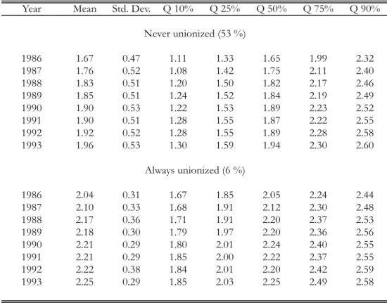
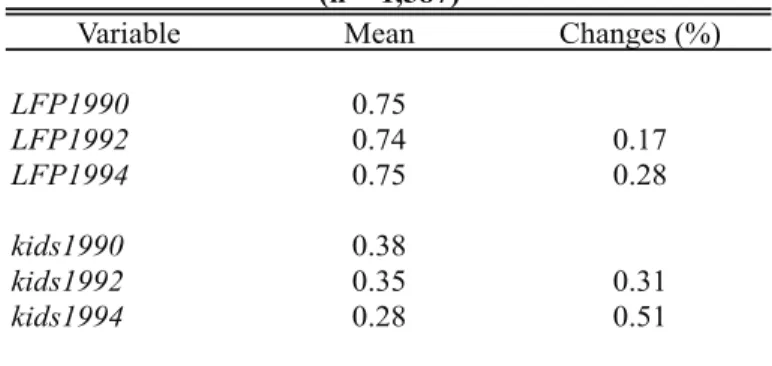
We give two empirical illustrations. One is to estimate the effect of unions on earnings quantiles. There we find that a decline in the union effect as the quantile increases can be attributed to individual heterogeneity. The other illustration is to estimate the effects of fertility on women’s labor force participation. There we compare nonparametric and semiparametric

estimates.

Recent research has considered nonseparable panel models with time homogeneity and con-tinuous regressors. Graham and Powell (2011) give estimators of the average effect in a linear model with heterogeneous slopes. Hoderlein and White (2011) give estimators of the average derivative conditional on equality of regressors across time periods.

Chamberlain (1980, 1984), Altonji and Matzkin (2005), Bester and Hansen (2008), and others have used control functions for panel data estimation. We focus instead on time homogeneity with unrestricted dependence between individual effects and regressors. Bias-corrected, fixed-effects estimation of semiparametric models has been proposed by Hahn and Kuersteiner (2002), Alvarez and Arellano (2003), Woutersen (2002), Hahn and Newey (2004), and Fern´andez-Val (2009). These estimators depend on large T for consistency while we estimate identified effects and bounds for fixed T .

Section 2 describes the models and effects we consider. Section 3 discusses estimation of identified effects. Sections 4 and 5 derive bounds for the static and dynamic nonparametric models respectively. Section 6 describes the impact of T . Section 7 describes and gives results for semiparametric, discrete-choice models. Section 8 gives computationally convenient methods for semiparametric models and numerical examples. Section 9 considers estimation and inference for semiparametric models. Section 10 gives empirical examples. The Supplementary Material Chernozhukov et. al. (2012) includes a variety of omitted discussions and results along with the proofs of results stated in the paper.

2

The Models and Effects

The data consist of n observations on Yi = (Yi1, ..., YiT)′ and Xi = [Xi1, ..., XiT]′, for a

depen-dent variable Yit and a vector of regressors Xit. Throughout we assume that the observations

(Yi, Xi), (i = 1, ..., n), are independent and identically distributed. The nonparametric models

we consider satisfy

Assumption 1: There is a function g0(x, α, ε) and vectors αi and εit of random variables

such that

Yit = g0(Xit, αi, εit), (i = 1, ..., n; t = 1, ..., T ).

The vector αi consists of time invariant individual effects that often represent individual

heterogeneity. The vector εitrepresents period-specific disturbances. Altonji and Matzkin (2005)

considered models satisfying Assumption 1. The invariance of g0 over time in this Assumption

be one of the components of εit, allowing the function to vary over time in a completely general

way. The next condition, together with Assumption 1, imposes time homogeneity on the model. Assumption 2: εit|Xi, αi = εd i1|Xi, αi, for all t.

This is a static, or “strictly exogenous” time homogeneity condition, where all leads and lags of the regressor are included in the conditioning variable Xi. It requires that the conditional

distribution of εitgiven Xiand αidoes not depend on t, but does allow for dependence of εitover

time. An equivalent condition is ˜εit|Xi = ˜εd i1|Xi for ˜εit= (αi, εit). Thus, the time invariant αihas

no distinct role in this model. The condition is just that whatever the unobserved disturbances are, their conditional distribution given Xi does not depend on t.

This seems a basic condition that helps panel data provide information about the effect of x on y. It is like “time is randomly assigned” or “time is an instrument” with the distribution of factors other than x not varying over time, so that changes in x over time can help identify the effect of x on y. Assumption 2 also turns out to be a natural strengthening of linear model conditions, as shown in Theorem A1 and the associated discussion in the Supplementary Material.

A dynamic model can be obtained by only including current and lagged Xis in the

condi-tioning set for each t, as in the following condition:

Assumption 3: εit|Xit, ..., Xi1, αi= εd i1|Xi1, αi, for all t.

This is a “predetermined” version of time homogeneity that is nested within the static model of Assumptions 1 and 2, as shown in Theorem A2 of the Supplementary Material. Here the conditional distribution given only current and lagged regressors must be time invariant. It also implies that the conditional distribution of εit given current and lagged regressors only

depends on Xi1. Here εit can be thought of as additional information that is independent of

the past regressors. A conditional-mean version of this condition arises in rational-expectations models that implies disturbances have mean zero conditional on past information. Here the stronger conditional independence restriction is imposed as seems needed for a nonseparable model. The conditioning on Xi1 is a way to account for the initial conditions of this dynamic

model. Bhargava and Sargan (1983) adopted this approach in a linear model as have Honore and Tamer (2006) and Browning and Carro (2007) in a likelihood setting.

If Xit includes lagged Yit then Assumption 3 specifies that the model is “dynamically

com-plete,” ruling out Yit = g0(Xit, αi, εit) as one equation of a dynamic system. For instance, Xit

could be Yi,t−1, in which case Yit = g0(Yit−1, αi, εit) is an explicit nonseparable dynamic model

where Yit ∈ {0, 1} is binary, representing state dependence, with αi representing unobserved

heterogeneity. This example is treated in Section 5.

We will focus in the nonparametric model on two objects, the average structural function (ASF) of Blundell and Powell (2003) and the quantile structural function (QSF) of Imbens and Newey (2009). The ASF is

µ(x) = E[g0(x, αi, εit)] =

Z

g0(x, α, ε)dF (α, ε),

where throughout the paper F denotes the cumulative distribution function (CDF) of a random vector that appears as the arguments of F . This object is useful for quantifying the effect of x on the mean of the outcome Yit. In the treatment-effects literature the average treatment effect

(ATE) of changing x from xb (before) to xa (after) is ∆ = µ(xa_{) − µ(x}b).

The QSF q(λ, x) is the λth quantile of g0(x, αi, εit). Under conditions specified below the

QSF will equal the inverse of the CDF of g0(x, αi, εit),

q(λ, x) = G−1(λ, x), G(y, x) = E[1(g0(x, αi, εit) ≤ y)].

In the treatment-effects literature the λth quantile treatment effect (QTE) of changing x from xb to xa is

∆λ = q(λ, xa) − q(λ, xb),

as in Lehmann (1974). This effect does not give the quantile of the treatment effect but does quantify the shift in the distribution of Yitthat is due to a change in x. It accounts for

multidi-mensional individual effects that may be correlated with x.

The static model implies a conditional-mean model that has been considered by Chamberlain (1982), Hahn (2001), Wooldridge (2005), and Chernozhukov et. al. (2007). This conditional-mean model specifies that there is an αi and m0(x, α) such that E[Yit|Xi, αi] = m0(Xit, αi). A

conditional mean ATE, as in Wooldridge (2005), isR [m0(xa, α) − m0(xb, α)]dF (α). This model

and effect differ from those we consider in specifying conditional-mean restrictions, while we specify conditional distribution restrictions. In Theorem A3 of the Supplementary Material we show that the conditional-mean model is implied by Assumptions 1 and 2, or 1 and 3, and that the conditional mean ATE is equal to the ATE we consider. Thus all results we give for the ATE, including bounds, apply to the conditional mean models, such as that of Chernozhukov et. al. (2007).

To help explain the relationship between the conditional-mean model and the model of our paper, and to illustrate other results, it is useful to consider examples. Binary choice is a very

important model for panel data, as it has many applications. For this reason we use binary choice as a main example. The most common model has been one with a scalar individual effect that is an additive shift to a linear combination of Xit, where

Yit= 1(Xit′ β∗+ αi ≥ εit),

for scalar εitand an unknown parameter vector β∗. In this example g0(x, α, ε) = 1(x′β∗+ α ≥ ε)

and the ATE is

∆ = Z

[1(xa′β∗_{+ α ≥ ε) − 1(x}b′β∗_{+ α ≥ ε)]dF (ε, α).}

This is an unusual object in the binary choice literature but is equal to a conditional mean ATE. In particular, if εit is independent of (Xi, αi) with CDF H(ε) for each t. Then E[Yit|Xi, αi] =

Pr(Yit = 1|Xi, αi) = H(Xit′ β∗+ αi) and

∆ = Z

[H(xa′β∗_{+ α) − H(x}b′β∗+ α)]dF (α).

Thus the ATE is also the effect of changing x on the choice probabilities averaged over the individual effect, i.e. the conditional mean ATE.

Our model also includes binary choice with individual-specific slopes as a special case. Eco-nomic motivation for varying slopes is provided by Browning and Carro (2007, 2009) who point out that with constant slopes the sign of the treatment effect is the same for every individual and give empirical examples where varying slopes are important. A general model with varying slopes is Yit= 1(X_it′αi ≥ εit) where Xitnow includes a constant and εitis independent of (Xi, αi)

with CDF H(ε). In this model ∆ =

Z

[H(xa′_{α) − H(x}b′α)]dF (α),

accounting for individual specific slopes. When Xit is discrete and fully saturated (e.g. consists

of a full set of dummies, one for every discrete outcome) this model is actually equivalent to the general static model. It will be more restrictive when the distribution of α is restricted in some way, such as having some components of α be constant. In the semiparametric analysis described below we show how to impose such restrictions.

Time effects are clearly important in practice but identification of treatment effects will preclude including t among the regressors Xit in the nonparametric model of Assumptions 1

- 3. Identification will be based on variation over time in Xit, and if t is a regressor then

g0(Xit, αi, εit) has unrestricted variation over time, precluding identification of the effect of any

other regressor. Some time effects can be allowed for by restricting the way t enters g0. Below

we will describe how this is done in semiparametric, discrete-choice models. With continuous Yit one can allow for location and scale time effects that are relatively easy to estimate.

Assumption 4: There is a function g0(x, α, ε), vectors αi and εit of random variables, and

constants τt, st, (t = 2, ..., T ) such that for τ1 = 0, s1 = 1,

Yit= gt0(Xit, αi, εit), gt0(x, α, ε) = τt+ stg0(x, α, ε), (i = 1, ..., n; t = 1, ..., T ).

This condition allows the mean and variance of Yit to vary over time in an unrestricted way.

The condition could be generalized to allow for other time effects, but we leave that to future work. It does not apply to Yit with fixed, discrete support because Assumption 4 does not make

sense in that case. There t must be included “inside” g0, as we do in the semiparametric analysis

described below.

With these time effects the ASF and QSF can depend on t. The ASF and QSF for the first period will be µ(x) and q(λ, x) as given above, and for the other periods are

µ_t(x) = τt+ stµ(x), qt(λ, x) = τt+ stq(λ, x), (t = 2, ..., T ).

Corresponding period-specific and time-averaged ATE and QTE are given by

µ_t(xa_{) − µt}(xb) = st[µ(xa) − µ(xb)], qt(λ, xa) − qt(λ, xb) = st[q(λ, xa) − q(λ, xb)], (1) PT t=1st T ! [µ(xa_{) − µ(x}b)], PT t=1st T ! [q(λ, xa_{) − q(λ, x}b)], where s1 = 1.

In the rest of this paper we will focus on discrete regressors, imposing the following condition from here on:

Assumption 5: The support of Xi is finite.

With discrete Xit the model can also be written as a multiple regression with random

coef-ficients, though we find it convenient to use the notation given here.

3

Identified Effects in the Nonparametric Static Model

The analysis of identification in the static model is quite simple. This simplicity is a virtue, leading to estimators of identified effects and bounds on unidentified effects that are easy to calculate in a very general model. For example, this approach gives a simple solution to the important problem of identification of quantile treatment effects in panel data. The idea is based on Assumption 2, which states that, conditional on Xi, the distribution of unobservables does

not vary over time. Therefore, conditional on Xi where both xb and xa occur for some time

periods, one can identify effects from the changes in Yit across those time periods. For the ATE,

subsets where both xb and xa occur for some time period. This idea is a slight extension of Chamberlain (1982, pp. 10-17) to discrete regressors that are not binary. For the QTE the distribution functions can be averaged and inverted to identify corresponding quantile effects. This idea appears to be novel.

There is a simple approach to allowing for covariates. Suppose x = (x1, x2), and one is

interested in the effect of x1 holding x2 fixed. Then one can take xb = (xb1, x2) and xa =

(xa₁, x2), so that the effect of changing from xb to xa is then the effect of interest. Furthermore,

one could average these effects over x2 to identify an effect that is averaged over covariates.

We explicitly allow for covariates in the semiparametric models given below. Because we are already attempting to cover so much ground here, we leave averaging over covariates in the nonparametric model to future work.

To describe identified effects and their estimators we will focus on the ATE and QTE condi-tional on both xa and xb appearing in Xi for some time period. We could also consider effects

conditional on smaller subsets of Xi but postpone this until later in order to keep the exposition

relatively simple. We need a little more notation to give a precise description. Let 1(Xit = x)

denote the indicator function that is equal to one when Xit = x and zero otherwise and let

Ti(x) =PTt=11(Xit= x). Here we let the subscript i denote a random variable that may depend

on Xi and Yi. Let Di = 1(Ti(xa) > 0)1(Ti(xb) > 0) be the indicator for the event that Xi

includes both xa and xb for some time period. Define

δ = E[g0(xa, αi, εi1) − g0(xb, αi, εi1)|Di= 1]. (2)

This δ is the ATE for those individuals where both xb _{and x}a_{occur for some time period. This}

effect may be of interest in many settings. For example, when Yitis log earnings and Xit∈ {0, 1}

represents union status, δ would be the average effect of union status on earnings for those who changed union status over the time periods we observe. For a given number of time periods T, this is all one could hope to identify nonparametrically. However, we may be interested in other effects too. We might be interested in union effects for those who ever changed union status at some time. This is δ. Or we might even be interested in the effect for those who were ever in a union. Bounds for such an effect are described below.

A simple estimator of the conditional ATE δ is ˆδ = Pn i=1Di[ ¯Yi(xa) − ¯Yi(xb)] Pn i=1Di , ¯Yi(x) = ( Ti(x)−1PTt=11(Xit = x)Yit, Ti(x) > 0 0, Ti(x) = 0 . (3) Consistency of this estimator results from

see Lemma A5 of the Supplementary Material. Intuitively, this equation follows from time being randomly assigned, so that we can estimate the effect by comparing Yit where Xit= xawith Yis

where Xis= xb.

Since ¯Yi(xa) − ¯Yi(xb) is a difference of means it can be interpreted as a coefficient of 1(Xit =

xa) in a regression of Yit on that dummy and on 1(Xit = xa) + 1(Xit = xb). Thus, ˆδ is

an average of least-squares estimates for each i with Di = 1. From this interpretation we

see that ˆδ extends Chamberlain’s (1982, p. 12) estimator to discrete regressors that are not binary. A consistent estimator of the asymptotic variance of √_{n(ˆδ − δ) is n}−1Pn

i=1ψˆ 2 i where

ˆ

ψ_i = nDi[ ¯Yi(xa) − ¯Yi(xb) − ˆδ]/Pn_i=1Di. For brevity we leave the asymptotic theory to the

Supplementary Material (see Theorem A6) and efficiency results to future work.

We can also identify and estimate a conditional QTE. Let G(y, x|Di= 1) = Pr(g0(x, αi, εi1) ≤

y|Di = 1) denote the CDF of g0(x, αi, εi1) conditional on Di = 1. The QTE conditional on

Di= 1 is

δλ = G−1(λ, xa|Di = 1) − G−1(λ, xb|Di = 1).

An estimator of this effect can be constructed using a CDF Φ(u) and a scalar bandwidth h. An estimator of G(y, x|Di = 1) is given by

ˆ G(y, x|Di = 1) = Pn i=1DiG¯i(y, x) Pn i=1Di , ¯Gi(y, x) = ( Ti(x)−1PT_t=11(Xit= x)Φ(y−Y_hit), Ti(x) > 0, 0, Ti(x) = 0. . In this estimator the indicator function 1(Yit < y) has been replaced by a smoothed

approxi-mation Φ(y−Yit

h ), as suggested by Yu and Jones (1998) for estimating a conditional CDF. An

estimator of δλ is then

ˆδλ = ˆqλa− ˆqbλ, ˆqaλ= ˆG−1(λ, xa|Di = 1), ˆqλb = ˆG−1(λ, xb|Di = 1).

Note here that we first average, then invert, and then difference. This estimator solves an important problem of estimating panel quantile effects and appears to be novel.

A consistent estimator of the asymptotic variance of √n(ˆδλ− δλ) is n−1Pni=1ψˆ 2 λi for ˆ ψ_{λi= −}PnDn i i=1Di " ¯ Gi(ˆqa, xa) − λ ˆ G′_(ˆqa_{, x}a_|D i = 1) − G¯i(ˆq b_{, x}b_{) − λ} ˆ G′_(ˆqb_{, x}b_|D i = 1) # ,

where ˆG′_{(y, x|D}i = 1) = ∂ ˆG(y, x|Di = 1)/∂y. Here the denominator terms are actually kernel

density estimates. For this reason one might use different bandwidths h in the numerator and denominator, with the denominator chosen to be appropriate for density estimation. Asymptotic theory for this estimator is given in the Supplementary Material (see Theorem A8). Alterna-tively, one could simply use the bootstrap to construct a confidence interval for ˆδλ.

A helpful example is the binary regressor case where Xit∈ {0, 1}. Here Xitcould be thought

of as a treatment variable where Xit = 1 for treated and Xit = 0 for untreated. Let Yit(0) =

g0(0, αi, εit) and Yit(1) = g0(1, αi, εit). Assumption 2 is equivalent to the assumption that

the conditional distribution of (Yit(0), Yit(1)) given Xi does not vary with t. This is the key

assumption that identifies treatment effects from time variation in treatment. In this context δ = E[Yit(1) −Yit(0)|Di = 1] is the ATE for individuals where both treatment and nontreatment

occurs during the observation period. Similarly, δλ is the difference between the λ quantile of

the distribution of Yit(1) and the λ quantile for Yit(0) conditional on Di = 1. The ATE and

QTE are not identified for those individuals that either receive treatment in every time period or receive no treatment in every time period.

In general the usual panel data within (linear fixed effects) estimator is not a consistent estimator of δ. This inconsistency results because the within estimator constrains the slope coefficient to be the same for each i when the slope is actually varying with i. For simplicity we demonstrate this inconsistency in the binary Xit example. The within estimator ˆδw is given by

ˆδw= Pn i=1 PT t=1(Xit− ¯Xi)Yit Pn i=1 PT t=1(Xit− ¯Xi)2 , ¯Xi = T−1 T X t=1 Xit. Let σ2 i = (T − 1)−1 PT

t=1(Xit− ¯Xi)2 be the sample variance over time of Xit.

Theorem 1: If Assumptions 1 and 2 are satisfied, Xit ∈ {0, 1}, E[Yit2] < ∞, (t = 1, ..., T ),

and E[Diσ2i] > 0, then δ = E[Di{ ¯Yi(1) − ¯Yi(0)}]/E[Di] and

ˆδw p −→ δw = E[σ2 iDi{ ¯Yi(1) − ¯Yi(0)}] E[σ2 iDi] . (4)

Note that the limit of the within estimator is a weighted average of individual, least-squares estimates ¯Yi(1) − ¯Yi(0) from equation (3). If T ≥ 4 then the weights σ2i vary over the positive

σ2_i and so the limit δw of ˆδw is not the identified conditional ATE δ.

Theorem 1 is different than Yitzhaki (1996) and Angrist (1998), who gave weighted average interpretations of least squares in other, non-panel settings. Theorem 1 is also different from Hahn (2001), who found that ˆδw consistently estimates the ATE. Hahn (2001) considered T = 2

and assumed Xi = (0, 1)′. As noted by Hahn (2001), those conditions are quite special. Theorem

1 is also different from Wooldridge (2005), who showed that if bi = E[Yit(1) − Yit(0)|αi] is mean

independent of Xit− ¯Xi for each t then linear fixed effects is a consistent estimator of δ. The

problem is that the mean-independence assumption is very strong when Xit is discrete. For

instance, if T = 2, Xi2 − ¯Xi takes on the values 0 when Xi = (1, 1) or (0, 0), −1/2 when

Xi = (1, 0) , and 1/2 when Xi = (0, 1). Thus mean independence of bi and Xi2− ¯Xi actually

implies that

This is quite close to independence of bi and Xi, which is not very interesting if we want to allow

the treatment effect to vary with Xi.

The conditional ATE and QTE estimators can easily be modified to accommodate the time effects of Assumption 4. The changes in Yit over time for fixed Xit can be used to identify and

estimate the time effects that can then be included in the estimation of the ATE and QTE. To describe this approach, let ˆmt=Pni=11(Xit= Xi1)Yit/Pni=11(Xit= Xi1) and

ˆ st= Pn i=11(Xit = Xi1)Xi1(Yit− ˆmt) Pn i=11(Xit = Xi1)Xi1(Yi1− ˆm1) , ˆτt= ˆmt− ˆstmˆ1, t = 2, ..., T.

This (ˆτt, ˆst)′ is an instrumental variables estimator where the residual is Yit− τt− stYi1, the

instruments are (1, Xi1)′, and the estimation is done on the subsample where Xit= Xi1. These

estimators will be consistent and asymptotically normal as long as Cov(Xi1, Yi1|Xit= Xi1) 6= 0

for each t = 2, ..., T. One could also use other functions of Xi1 as instrumental variables to

improve efficiency. We focus on just Xi1 as an instrument for simplicity. Graham and Powell

(2011) use a similar approach to identify time effects in a linear model with continuous regressors. The time effects are accounted for in ATE and QTE estimation by removing time location and scale effects from all periods when estimating the first period effect, and then putting the scale effects back for other periods. Note first that under Assumption 4 δ is the conditional ATE for the first time period. Let ˜Yit = (Yit− ˆµt)/ˆst be the tth period observation with estimated

location and scale removed. Replacing Yit by ˜Yit in the formula for ˆδ gives

˜δ = Pn i=1Di[ ˜Yi(xa) − ˜Yi(xb)] Pn i=1Di , ˜Yi(x) = ( Ti(x)−1PTt=11(Xit = x) ˜Yit, Ti(x) > 0 0, Ti(x) = 0 .

The conditional ATE for the tth_{time period is given by s}

tδ and a time average by (PTt=1st/T )δ

for s1 = 1, analogously to equation (1). These can be estimated by ˆst˜δ and ¯s˜δ, respectively

for ¯s =PT

t=1ˆst/T and ˆs1 = 1. These estimators will be consistent and asymptotically normal.

Because of their multistage nature the bootstrap may provide the easiest approach to carrying out inference on these estimators, where one resamples from the empirical distribution of (Yi, Xi),

(i = 1, ..., n) to form confidence intervals for the true parameter. For brevity we omit explicit results.

An analogous approach can be followed to account for time effects in the QTE. The inter-pretation of δλ now becomes QTE for the first time period conditional on Di = 1. An estimator

of G(y, x|Di = 1) = Pr(g0(x, αi, εi1) ≤ y|Di = 1) that adjusts for time, location and scale is

given by ˜ G(y, x|Di = 1) = Pn i=1DiG˜i(y, x) Pn i=1Di , ˜Gi(y, x) = ( Ti(x)−1PTt=11(Xit = x)Φ(y− ˜_hYit), Ti(x) > 0 0, Ti(x) = 0 .

Let ˜qa_λ= ˜G−1(λ, xa_|Di = 1) and ˜qλb = ˜G−1(λ, xb|Di = 1). Estimators for the conditional QTE for

the first period, other periods, and a time average are given by ˜δλ = ˜qaλ− ˜qλb, ˆst˜δλ, (t = 2, ..., T ),

and ¯s˜δλ, respectively. Here again the bootstrap provides a convenient method for inference. One

could also use quantiles to estimate the time effects, but we avoid that for simplicity.

4

Nonparametric Bounds in the Static Model

When g0(x, αi, εit) is bounded we can estimate bounds for the ASF and corresponding bounds

for the ATE. For the QSF and QTE we can also estimate bounds without any restriction on g0, using the fact that there are known upper and lower bounds for the indicator function

1(g0(x, αi, εit) ≤ y). The idea of the bounds is an extension of the estimation of identified effects

discussed in the previous Section. Time homogeneity allows us to use time averages to estimate the identified parts of the ASF or QSF when x is an element of Xi, i.e. Xit = x for some t, and

apply the lower or upper bounds when x does not appear in Xi.

We first describe bounds estimation for the ASF. These bounds depend on bounds on g0

imposed in the following condition:

Assumption 6: Bℓ ≤ g0(x, αi, εit) ≤ Bu for constants Bℓ and Bu and all x.

For example, in the binary-choice model, where Yit ∈ {0, 1}, upper and lower bounds are

Bu = 1 and Bℓ = 0 respectively. We could allow Bℓ and Bu to depend on x and using that

information could tighten the ATE bounds given below. To avoid further complication we do not allow this.

Let Ti(x) and ¯Yi(x) be as in Section 3 and ¯P (x) = Pni=11(Ti(x) = 0)/n be the sample

frequency of x not occurring in any time period. Estimated lower and upper bounds for µ(x) are ˆ µ_ℓ(x) = n−1 n X i=1 ¯ Yi(x) + ¯P (x)Bℓ, ˆµu(x) = ˆµℓ(x) + ¯P (x)(Bu− Bℓ).

Here ¯Yi(x) estimates the identified part of the ASF, corresponding to Ti(x) > 0, and the upper

and lower bounds are applied for observations where Ti(x) = 0 . Corresponding estimated lower

and upper bounds for the ATE are ˆ∆ℓ = ˆµℓ(xa) − ˆµu(xb) and ˆ∆u = ˆµu(xa) − ˆµℓ(xb). The width

of these estimated bounds is ˆ

∆u− ˆ∆ℓ= [ ¯P (xa) + ¯P (xb)](Bu− Bℓ).

For example, for binary choice with a binary regressor, where Bu = 1 and Bℓ = 0, the width

of the estimated bounds for the ATE is ¯P (0) + ¯P (1), where ¯P (0) and ¯P (1) are the sample proportions of Xi with Xit = 1 for all t and Xit= 0 for all t, respectively

These estimators will be jointly asymptotically normal under i.i.d. (Yi, Xi). The asymptotic

variance can be estimated by ˆΣ =Pn

i=1ΨˆiΨˆ′i/n, where ˆ Ψi= ¯ Yi(xa) − ¯Yi(xb) + Bℓ1(Ti(xa) = 0) − Bu1(Ti(xb) = 0) − ˆ∆ℓ ¯ Yi(xa) − ¯Yi(xb) + Bu1(Ti(xa) = 0) − Bℓ1(Ti(xb) = 0) − ˆ∆u ! .

Confidence intervals for the identified set can then be formed using results of Chernozhukov, Hong, and Tamer (2007) or Beresteanu and Molinari (2008, pp. 779-781) on estimators of intervals where the upper and lower endpoints are jointly asymptotically normal.

Turning to the bounds for the QSF, lower and upper estimated bounds for the G(y, x) = Pr(g0(x, αi, εi1) ≤ y) are ˆGℓ(y, x) =Pi=1n G¯i(y, x)/n and ˆGu(y, x) = ˆGℓ(y, x)+ ¯P (x) respectively.

The idea of these bounds is similar to the ASF, with a known lower bound of 0 and upper bound of 1 for 1(g0(x, αi, εi1) ≤ y). To obtain quantile bounds we need to invert these functions of y.

For a strictly increasing function G(y) with range contained in [0, 1] let

Q(λ, G(·)) =        −∞, λ ≤ infyG(y) G−1_{(λ), inf}

yG(y) < λ < supyG(y)

+∞, λ ≥ supyG(y)

.

This is a function with domain [0, 1] and range equal to the extended real line that can be used to invert ˆGu(y, x) and ˆGℓ(y, x). Estimators of lower and upper bounds on the QSF are given by

ˆ

qℓ(λ, x) = Q(λ, ˆGu(·, x)), ˆqu(λ, x) = Q(λ, ˆGℓ(·, x)).

Corresponding lower and upper bounds for the QTE are ˆ∆λℓ = ˆqaℓ− ˆqub and ˆ∆λu= ˆqau− ˆqℓbwhere

ˆ qa

ℓ = ˆqℓ(λ, xa), ˆqau = ˆqu(λ, xa), ˆq_ℓb = ˆqℓ(λ, xb), and ˆqub = ˆqu(λ, xb). The width of these bounds

depends on the shape of the empirical distribution of Yit and on ¯P (x). The width of the bounds

will be finite when

max{ ¯P (xa), ¯P (xb_{)} < λ < min{1 − ¯}P (xa_{), 1 − ¯}P (xb_)}, (5) and otherwise they are infinitely wide.

The bounds will be joint asymptotically normal under the following regularity condition: Assumption 7: Pr(g0(x, αi, εi1) ≤ y|Xi) is twice continuously differentiable in y with

uni-formly bounded derivatives and Gℓ(y, x) = E[E[1(Ti(x) > 0)|Xi] Pr(g0(x, αi, εi1) ≤ y|Xi)] is

strictly increasing in y on the interior of its range for all x. Also nh4 _{−→ 0 and nh}2 _{−→ ∞.} For λ satisfying equation (5) the asymptotic variance can be estimated by ˆΣλ =Pni=1ΨˆλiΨˆ′_λi/n,

where ˆ Ψλi=   ¯ Gi(ˆqaℓ,xa)+1(Ti(xa)=0)−λ ˆ G′ ℓ(ˆq a ℓ,xa) − ¯ Gi(ˆqbu,xb)−λ ˆ G′ ℓ(ˆqbu,xb) ¯ Gi(ˆqau,xa)−λ ˆ G′ u(ˆqau,xa) − ¯ Gi(ˆqbℓ,xb)+1(Ti(xb)=0)−λ ˆ G′ ℓ(ˆq b ℓ,xb)  .

As in estimation of the conditional quantile effect, one might want to use different bandwidths for numerators and denominators, or just bootstrap to estimate the asymptotic variance.

Here is a result for both ATE and QTE bounds:

Theorem 2: Suppose that Assumptions 1, 2, and 5 are satisfied. If Assumption 6 is satisfied then there are ∆ℓ, ∆u, and Σ such that

√

n[( ˆ∆ℓ, ˆ∆u)′− (∆ℓ, ∆u)′]−→ N(0, Σ), ˆd Σ−→ Σ.p

where ∆ℓ ≤ ∆ ≤ ∆u, and these bounds are sharp. If Assumption 7 is satisfied then there are

∆λℓ, ∆λu, and Σλ such that

√

n[( ˆ∆λℓ, ˆ∆λu)′− (∆λℓ, ∆λu)′]−→ N(0, Σd λ), ˆΣλ p

−→ Σλ.

where ∆λℓ ≤ ∆λ ≤ ∆λu. If Gℓ(y, x) is also everywhere strictly increasing in y then these

bounds are sharp.

The sharpness conclusion of Theorem 2 for the ATE depends on being able to let g0(x, αi, εit)

take any value between Bℓand Bu. That is not possible for binary choice, where the outcome is

restricted to zero or one. Nevertheless the bounds can still be shown to be sharp.

Similarly to the treatment-effects literature, we may be interested in the ATE or QTE, conditional on Xi ∈ S for some set S. For example, if Xit ∈ {0, 1} represents treatment then

we might be interested in the effect of treatment conditional on ever treated, i.e. conditional on Xi6= (0, ..., 0)′. Tighter bounds for such effects can be formed and in some cases the effects may

be identified. These bounds can be estimated by replacing 1(Xit = x) by 1(Xi ∈ S)1(Xit = x)

in the definition of ¯Yi(x) and ¯Gi(y, x), 1(Ti(x) = 0) by 1(Xi ∈ S)1(Ti(x) = 0) in the definition

of ¯P (x), and dividing through by Pn

i=11(Xi ∈ S)/n. If 1(Xi ∈ S) ≤ Di for Di from Section 3

the corresponding effects will be identified, and the upper and lower estimated bounds will be identical.

Time effects can easily be allowed for in quantile-effect bounds by adapting the approach used earlier. It is not clear that allowing for time effects in that way makes sense for bounds on the ATE, e.g. for binary choice models where the support of Yitis fixed. Therefore we focus just

on time effects in quantile bounds. For QTE bounds we can replace Yit by ˜Yit = (Yit− ˆµt)/ˆst

in the formula for ˆGℓ(y, x) given above, and interpret ˆ∆λℓ and ˆ∆λu as estimators of the first

period bounds. Estimators of tth period lower and upper bounds for the QTE are then given by ˆst∆ˆλℓand ˆst∆ˆλurespectively. Estimators of time average bounds are ¯s ˆ∆λℓ and ¯s ˆ∆λu, where

¯ s = PT

t=1sˆt/T. These upper and lower bounds will be joint asymptotically normal, and their

5

Nonparametric Bounds in the Dynamic Model

Analysis of the dynamic model is more challenging than that of the static one. In the dynamic model of Assumption 3 only the first-period regressor is common to the conditioning sets for each time period. Consequently location and scale time effects are not identified, because the conditioning set is different for every time period. For this reason we do not consider time effects in the nonparametric dynamic model. Also, the identification and bounds analysis is limited to objects that are conditional on the first period or are unconditional. For example, we cannot identify or bound the ATE conditional on Xit changing over time because that event

involves information about all time periods. We can bound unconditional objects and ones that are conditional on just Xi1. These bounds are simple and novel, for example in providing

partial-identification results for the average effect of state dependence with heterogeneity in both location and slope when Yit is binary and Xit= Yit−1.

The model with a binary, lagged dependent variable has Yit = g0(Yi,t−1, αi, εit), and under

Assumption 3,

Pr(Yit= 1|Xit, ..., Xi1, αi) =

Z

g(Yi,t−1, αi, ε)dF (ε|αi, Yi0)

= Pr(Yit= 1|Yi,t−1, αi, Yi0),

where F (ε|αi, Yi0) denotes the conditional CDF of εitgiven αiand Yi0. Here Pr(Yit= 1|Yi,t−1, αi, Yi0)

does not vary with t, and the model places no other restrictions on Pr(Yit = 1|Yi,t−1, αi, Yi0).

Conditioning on Yi0 is present to account correctly for the initial condition, as in Honore and

Tamer (2006) and Browning and Carro (2007, 2009). The probabilities can be distributed across individuals in any way at all through the individual effect αi. That is we can think of the four

conditional probabilities,

Pr(Yit= 1|1, αi, 1), Pr(Yit = 1|0, αi, 1) Pr(Yit= 1|1, αi, 0), Pr(Yit = 1|0, αi, 0),

as having an unrestricted distribution. Here the ATE is ∆ =

Z

[Pr(Yit = 1|Yi,t−1= 1, α, Y0) − Pr(Yit= 1|Yi,t−1= 0, α, Y0)]dF (α, Y0).

This object quantifies the effect of state dependence in the presence of individual heterogeneity, an important problem posed by Feller (1943) and Heckman (1981). The dynamic bounds here provide a simple, estimable, identified set for this object. This model is considered by Browning and Carro (2007, 2009), who derive properties of various estimators and restrictions on αi that

lead to identification. We give nonparametric bounds.

A partition of Xi values that preserves the dynamic structure of Assumption 3 is used to

first occurrence of x is at time t and the set where x never occurs. This partition is given by { ¯X (x), X1(x), ..., XT(x)} where

Xt(x) = {X : Xt= x, Xs6= x ∀s < t}, t = 1, ..., T ; ¯X (x) = {X : Xt 6= x ∀t}.

Define ˆYi(x) =PTt=11(Xi∈ Xt(x))Yit, which picks out the Yit for the time period where x first

occurs. Estimated lower and upper ASF bounds are ˆ µ_ℓ(x) = n−1 n X i=1 ˆ Yi(x) + ¯P (x)Bℓ, ˆµu(x) = ˆµℓ(x) + ¯P (x)(Bu− Bℓ).

Corresponding lower and upper bounds for ∆ are ˆ∆ℓ = ˆµℓ(xa)−ˆµu(xb) and ˆ∆u= ˆµu(xa)−ˆµℓ(xb).

A joint asymptotic-variance estimator ˆΣ can be constructed exactly as for the static case with ˆ

Yi(x) replacing ¯Yi(x).

It is interesting to note that the width ¯P (x)(Bu − Bℓ) of the estimated ASF bounds is the

same for the dynamic and static models. Because the static model is a special case of the dynamic one we conjecture that the bounds for the dynamic model are sharp like the bounds for the static one, but have not yet been able to show this.

To construct estimated lower and upper bounds for the CDF of g0(x, αi, εit) let ˆGi(y, x) =

PT

t=11(Xi ∈ Xt(x))Φ(y−Y_hit). The estimated CDF bounds are

ˆ Gℓ(y, x) = 1 n n X i=1 ˆ

Gi(y, x), ˆGu(y, x) = ˆGℓ(y, x) + ¯P (x).

Estimated lower and upper bounds for the QSF are then given by ˆ

qℓ(λ, x) = Q(λ, ˆGu(·, x)), ˆqu(λ, x) = Q(λ, ˆGℓ(·, x)).

Corresponding lower and upper bounds for the QTE are ˆ∆λℓ= ˆqℓ(λ, xa) − ˆqu(λ, xb) and ˆ∆λu=

ˆ

qu(λ, xa) − ˆqℓ(λ, xb). A joint asymptotic variance estimator ˆΣλ can be constructed just as for the

static case with ˆGi(y, x) replacing ¯Gi(y, x).

Theorem 3: Suppose that Assumptions 1, 3, and 5 are satisfied. If Assumption 6 is satisfied then there are ∆ℓ, ∆u, and Σ such that

√

n[( ˆ∆ℓ, ˆ∆u)′− (∆ℓ, ∆u)′]−→ N(0, Σ), ˆd Σ p

−→ Σ.

where ∆ℓ ≤ ∆ ≤ ∆u. Also if Assumption 7 is satisfied with Xi1 replacing Xi then there are

∆λℓ, ∆λu, and Σλ such that

√

n[( ˆ∆λℓ, ˆ∆λu)′− (∆λℓ, ∆λu)′]−→ N(0, Σd λ), ˆΣλ p

−→ Σλ.

Similarly to the static model we may be interested in effects conditional on Xi1∈ S1for some

set S1. For example, if Xit ∈ {0, 1} represents treatment then we might be interested in the effect

of treatment conditional on being treated in the first period, i.e. conditional on Xi1= 1. Tighter

bounds for such effects can be estimated by replacing 1(Xi ∈ Xt(x)) by 1(Xi1∈ S1)1(Xi ∈ Xt(x))

in the definition of ˆYi(x) and ˆGi(y, x), 1(Ti(x) = 0) by 1(Xi1∈ S1)1(Ti(x) = 0) in the definition

of ¯P (x), and dividing through byPn

i=11(Xi1∈ S1)/n.

In the binary, lagged-dependent-variable example we have Bℓ= 0 and Bu = 1, so the bounds

on the ATE are ˆ ∆ℓ = 1 n n X i=1 [ ˆYi(1) − ˆYi(0)] − ¯P (0), ˆ∆u = ˆ∆ℓ+ ¯P (1) + ¯P (0).

Here ¯P (1) + ¯P (0) estimates the width of the bounds, providing a very simple measure of the severity of the problem of identifying state dependence in the presence of heterogeneity. The bounds will tend to be wide in short panels but more informative in long ones.

Figure 1 shows the width of corresponding population bounds in a numerical example based on a dynamic probit model where

Yit= 1(β∗Yi,t−1+ αi ≥ εit), εit∼ N(0, 1), αi∼ N(0, 1), Pr(Yi0= 1) = .5.

We consider different DGPs indexed by β∗ _{∈ [−2, 2] and compute the width of the bounds} for T ∈ {2, 4, 8, 16, 32, 64}. The width is asymmetric with respect to β∗ = 0 because Pr(Xi =

(1, ..., 1)′) grows with β∗, whereas Pr(Xi= (0, ..., 0)′) does not depend on β∗. The width growing

with β∗ may therefore be explained by having fewer switches of Yit between one and zero when

β∗ is larger. It is presumably the changes that help identify the ATE. We find that the bounds can be substantially wide for high values of β∗ even for large T , consistent with the width of the nonparametric bounds shrinking only at rate 1/T, as shown in the next Section. Semiparametric bounds for this model that impose the constancy of β∗across individuals, will shrink much faster at T grows, as shown in Section 7.

6

_{The Impact of T}

Increasing T improves identification, shrinking the estimated and population-identified sets for the objects of interest. The rate at which the identified set shrinks quantifies this improvement. Here we give rates for the ASF and, for brevity, leave the quantile results to the Supplementary Material.

The width of the population bounds for the ASF is (Bu− Bℓ) ¯P(x) where

¯

Thus, the rate at which the identified set shrinks, that we will refer to as the identification rate, is the same as the rate at which ¯_{P(x) shrinks. Factors that determine this rate can be seen} when Xit is i.i.d. conditional on αi. In that case

¯

P(x) = E[Pr(Xit6= x|αi)T].

The rate at which ¯_{P(x) goes to zero will be determined by how much probability mass of} Pr(Xit 6= x|αi) is close to one. If Pr(Xit 6= x|αi) = 1 with positive probability then ¯P(x) does

not go to zero. This corresponds to nonidentification of the ASF, where x does not occur for some individuals as indexed by αi (see Theorem A11 of the Supplementary Material). On the

other hand, if Pr(Xit 6= x|αi) is bounded away from one then the identified set will shrink

exponentially quickly, since Pr(Xit 6= x|αi)T ≤ (1 − ε)T for some ε > 0. In between the

nonidentified and exponential rate cases there are a range of rates depending on how much of the distribution of Pr(Xit 6= x|αi) is close to 1. The following result shows the range of rates.

Theorem 4: Suppose that Assumptions 1, 3, 5, and 6 are satisfied and (Xi1, Xi2, ...) is

sta-tionary and Markov of order J conditional on αi. If for some ε > 0, Pr(Xit= x|Xi,t−1, ..., Xi,t−J, αi) ≥

ε a.s. then µ_{u(x)−µℓ(x) ≤ (B}u−Bℓ)(1−ε)T −J. If Xitis i.i.d. conditional on αi, Pr(Xit6= x|αi)

is continuously distributed with pdf fP(p), and

fP(p) ≤ Cpγ−1(1 − p)v−1, γ > 0, v > 0, (6)

then µ_{u(x) − µℓ}(x) = O(T−v).

The upper bound on the rate at which the pdf fP(p) of Pr(Xit 6= x|αi) grows or converges

to zero as p −→ 1 provides an upper bound on the rate at which the identified set shrinks. For example, if v = 1 so that fP(p) is bounded as p −→ 1, then the identified set shrinks at rate

1/T. All of the rates implied by this result are slower than the exponential rate, reflecting how having Pr(Xit 6= x|αi) close to 1 affects the rate. Also, γ has no effect on the convergence rate

because that rate is determined by closeness of Pr(Xit6= x|αi) to 1, and not to 0.

The dynamic, binary-choice model is an example where more explicit conditions can be given. Suppose Yit= 1(αi1+ (αi2− αi1)Yi,t−1≥ εit) and εit is i.i.d. and independent of αi= (αi1, αi2)

with CDF H(ε). Here Pr(Yit = 1|Yi,t−1 = 0, αi) = H(αi1) and Pr(Yit = 1|Yi,t−1 = 1, αi) =

H(αi2). Unbounded αi and bounded εit will correspond to the unidentified case. Bounded αi

and unbounded εit lead to an exponential convergence rate. The following result covers the

in-between case. Let fε(ε), fα1(α), and fα2(α) denote the pdfs of εit, αi1, and αi2 respectively,

Theorem 5: If Yit = 1(αi1+ (αi2− αi1)Yi,t−1 ≥ εit), where εit, (t = 1, ..., T ) is i.i.d. and

independent of (αi1, αi2) and there is v, C > 0 such that for all ε

max

j=1,2fαj(ε) ≤ CH(ε)

v−1_{[1 − H(ε)]}v−1_f

ε(ε), (7)

then ∆u− ∆ℓ = O(T−v).

Here we see that the identification rate in the nonparametric dynamic model is related to the tail thickness of the distribution of αi1 and αi2 relative to the distribution of εit. The thinner

the tail of fε(ε) relative to the tails of fα1(α1) and fα2(α2) the smaller v will need to be to

satisfy the inequality in Theorem 5 and the slower the identification rate will be. In this way the identification rate is slower the less strong the signal provided by εit relative to the individual

effects. Here there is no γ present because both left and right tails matter, in order to bound the rate for the ATE, and not just for the ASF at a particular x.

For a specific example consider αi1 and αi2 as N (0, σ2α) and εit as N (0, σ2ε) where σ2ε ≤ σ2α.

Then for constants C1, C2, and v = σ2ε/σα2 we have fαj(ε) = C1[fε(ε)]

v_{. Also, as is well known}

for the Gaussian distribution, fε(ε) ≥ C2Fε(ε)[1 − Fε(ε)], where Fε(ε) denotes the CDF of ε. It

follows by v ≤ 1 that

fαj(ε) = C1[fε(ε)]

v−1_f

ε(ε) ≤ C1C2v−1Fε(ε)v−1[1 − Fε(ε)]v−1fε(ε).

Thus equation (7) is satisfied with v = σ2_ε/σ2_α so that ∆u− ∆ℓ= O(T−σ

2 ε/σ2α_).

Hence the width of the bounds shrinks at a rate no larger than T−1 and the rate is slower the smaller σ2

ε/σ2α is. It can also be shown that convergence is faster than T−1 when σ2ε > σ2α and

increases with σ2_ε/σ2_α. Thus we see that the stronger the signal provided by ε relative to that provided by α, in the sense that the higher σ2

εis relative to σ2α, the faster will be the identification

rate.

One can obtain analogous results in a static model. If Xit= 1(αi ≥ ηit) is a binary regressor

where η_it is i.i.d. over time then the identification rate will be T−v _{when the inequality in}

Theorem 5 is satisfied with the pdf fη(η) of ηitreplacing the pdf fε(ε). If αiand ηitare distributed

as N (0, σ2

α) and ηitas N (0, σ2η) respectively with σ2η ≤ σ2α, then the identified set shrinks at rate

T−σ2η/σ2α_{. For brevity we omit the details.}

7

Semiparametric Multinomial Choice Models

The nonparametric bounds are informative but may be quite wide for small T . They can be tightened by imposing additional structure on the model. One way to do this is to specify a

parametric model for the conditional distribution of Yi given values for (Xi, αi). We focus here

on multinomial choice models. In those models Yi is one of a finite number of outcomes, denoted

here by {Y1, ..., YJ_{}. The parametric part of the model are the known conditional probabilities} Lk

j(α, β) of Yi = Yj given αi and Xi ∈ Xk, (k = 1, ..., K), where β is a parameter vector with

true value β∗_{, and X}k is the set of Xi values being conditioned on. Formulating the model

in this way allows for Xi that are lagged dependent variables. The nonparametric part of the

model will be the unknown CDF’s F_k∗(α), (k = 1, ..., K) of αi conditional on Xi in each Xk. The

model then satisfies

Assumption 8: Pr(Yi = Yj|Xi ∈ Xk) =R Lkj(α, β∗)dFk∗(α), (j = 1, ..., J; k = 1, ..., K).

Some examples may be helpful. An important example is a binary choice model where Yit∈ {0, 1}, α is a scalar location individual effect, Pr(Yit= 1|Xi, αi, β∗) = H(Xit′ β∗+ αi) for a

CDF H(ε), and Yi1, ..., YiT are mutually independent conditional on Xi and αi. In this case we

would let Xk be a singleton given by the kth value Xk in the finite support of Xi and

Lkj(α, β) = T Y t=1 H(X_tk′β + α)Ytj[1 − H(Xk′ t β + α)]1−Y j t. (8)

Time effects can be included in this model by specifying that some components of Xk

t only depend

on t. This model can also be generalized to allow for some slopes to vary across individuals by specifying that Lkj (α, β) = T Y t=1 H(z′_tβ₁+ X_t1k′β₂+ X_t2k′α)Ytj_{[1 − H(z}′ tβ1+ Xt1k′β2+ Xt2k′α)]1−Y j t _{. (9)}

This model allows the coefficients of X_t2k to vary with individuals, which will include a location effect when some element of Xk

t2 does not vary with t or k.

This set up also allows for dynamic models. For example, consider a binary choice model with a lagged dependent variable where Pr(Yit= 1|Yi,t−1, ..., Yi0, αi, β∗) = H(Yi,t−1β∗+αi). Here

Xi= (Yi,T −1, ..., Yi0) and we take K = 2, with Xk = {Xi : Xi1= Yi0= k − 1}. The parametric

part of the model is

Lkj(α, β) = T Y t=2 H(Y_t−1j β + α)Ytj[1 − H(Yj t−1β + α)]1−Y j t (10) ×H((k − 1)β + α)Y1j[1 − H((k − 1)β + α)]1−Y j 1.

This model could be generalized to allow individual specific coefficients for the dynamic effect, time effects, and other covariates, including the model of Browning and Carro (2009). For brevity we omit this generalization.

The ATE and its bounds can be decomposed into a weighted average of conditional ATE and corresponding bounds, weighted by the identified Pr(Xi ∈ Xk). The semiparametric model

may restrict the conditional bounds so we focus first on them. We will assume that a conditional ATE takes the form

∆k= Z

∆(α, β∗)dF_k∗(α),

where ∆(α, β) denotes a treatment effect conditional on α. For example, in the model of equation (8) we could take ∆(α, β) = H(xa′_{β + α) − H(x}b′_{β + α), in which case}

∆k= Z

[H(xa′β∗_{+ α) − H(x}b′β∗+ α)]dF_k∗(α)

is the ATE conditional on Xi = Xk. One could also consider the ASF conditional on Xi = Xk,

that would beR H(x′_β∗_{+ α)dF}∗

k(α) in this example.

Neither ∆k _{nor β}∗ _{need be identified. Instead, there may be sets of β}∗ _{and ATE values}

that are consistent with the distribution of the data. To describe the identified sets let P = (P11, ..., PJ1, ..., PJK)′ denote the vector of population choice probabilities with Pjk = Pr(Yi =

Yj_|Xi∈ Xk) and

Fk(β, P) = {Fk : Pjk =

Z

Lkj (α, β) dFk(α), j = 1, ..., J},

where Fk(β, P) may be empty. The identified set for β∗ is

B = {β s.t. Fk(β, P) 6= ∅, ∀k = 1, ..., K}.

That is, B is the set where there exist individual effect distributions such that integrals of model probabilities equal population choice probabilities. Sharp upper and lower bounds ∆k

u and ∆kℓ

for ∆k are given by ∆k_u= sup β∈B,Fk∈Fk(β,P) Z ∆(α, β)dFk(α) , ∆kℓ = inf β∈B,Fk∈Fk(β,P) Z ∆(α, β)dFk(α) . (11)

This characterization of bounds for the ATE extends that of Honore and Tamer (2006) from a finite dimensional Fk, where α is restricted to a known fixed grid, to infinite-dimensional Fk

where any distribution for α is allowed.

For purposes of comparison with the nonparametric results we consider models without trends, where the semiparametric models in equations (8) and (10) are nested in the nonpara-metric static or dynamic model. In those models ∆k will be identified if it is also identified in the nonparametric model. In the static case ∆k is nonparametrically identified if X_tk takes on the values xb _{and x}a _{for some time periods. This follows similarly to the identification of the}

by imposing the restrictions of a semiparametric model is limited to those ∆k where at least one of xb _{or x}a _{does not appear in any time period. In what follows we focus on these ∆}k_.

When slopes vary across individuals the semiparametric bounds may be no tighter than the nonparametric ones. To illustrate consider a binary-choice model with a single binary regressor Xit, where Yit= 1((αi2−αi1)Xit+αi1> εit), εitis independent of (Xi, αi2, αi1), and εithas known

CDF H(ε) that is strictly increasing on the entire real line. The joint distribution of H(αi1)

and H(αi2) conditional on Xi = Xk is entirely unrestricted. Therefore when Xk = (0, ..., 0)′

the fact that E[H(αi1)|Xi = Xk] = E[Yit|Xi = Xk] for every every t, and so is identified gives

no information about E[H(αi2)|Xi = Xk]. Thus, E[H(αi2)|Xi = Xk] can be anything in the

unit interval. Therefore, the width of the bound for ∆k= E[H(αi2) − H(αi1)|Xi = Xk] will be

equal to the width in the nonparametric case, ∆k

u− ∆kℓ = 1. More generally, in the panel binary

choice model of equation (9), when there are no time effects, every coefficient of Xitvaries across

individuals, and Xit is fully saturated (e.g. is a complete set of dummies, one for every possible

value of Xit), the semiparametric bounds will equal the nonparametric ones.

In the binary-regressor case the width of the overall bound on the ATE is given by

∆u− ∆ℓ= ¯P(0)(∆1u− ∆ℓ1) + ¯P(1)(∆2u− ∆2ℓ). (12)

where we assume X1 _{= (0, ..., 0)}′ _{and X}2 _{= (1, ..., 1)}′_{. The semiparametric bounds will be}

smaller than the nonparametric bounds if and only if ∆1_{u− ∆}1_ℓ or ∆2_{u− ∆}2_ℓ are smaller than the nonparametric values of 1. This decomposition also shows that the semiparametric identification rate will be determined by the nonparametric rate, which governs how fast ¯_{P(0) and ¯P(1)} shrink, and the rate that the conditional bounds converge. When the slope does not vary across individuals it turns out that the conditional bounds can converge very rapidly. The following result shows this in static and dynamic, binary-choice logit models with binary regressors.

Theorem 6: Suppose that H(v) = ev_{/(1 + e}v_{), ∆(β, α) = H(β + α) − H(α), and either}

equation (8) is satisfied with, Xit∈ {0, 1}, and X1 = (0, ..., 0)′ and X2 = (1, ..., 1)′, or equation

(10) is satisfied with k ∈ {1, 2}. Then there are C > 0 and 1 > ε > 0 such that ∆k_{u− ∆}k_{ℓ ≤ C(1 − ε)}T, k = 1, 2.

This fast rate occurs because T conditional moments of a one-to-one transformation of αi are

identified from probabilities of various Y values, and these moments lead to a fast approximation of the conditional ATE. For example, Pr(Yi = (1, ..., 1)′|Xi = X1) = E[H(αi)T|Xi = X1], and

other conditional moments of H(αi) can be similarly identified. For the logit H(α), identification

of these moments leads to fast approximation of ∆1 _{= E[H(β}∗ _{+ α}

i) − H(αi)|Xi = X1] and

From equation (12) we see that the semiparametric identification rate in this example will be at least exponential, and may be even faster, depending on the nonparametric rate. This result illustrates how imposing a single, additive individual effect can speed up the identification rate. We expect that this type of improvement will extend beyond the logit model with binary regressors.

8

Computation of Semiparametric Bounds

In this section we discuss computation of population bounds, give examples, and present the-oretical results. A challenge for computation and for estimation is the dimensionality of the unknown parameters and the nonlinearity of the probabilities in those parameters. A useful feature of multinomial panel models is that they are finite dimensional, in spite of the presence of distributions. The following lemma shows that one only need consider discrete distributions with J unknown support points in the specification of the likelihood and the bounds for the ATE. Let Υ denote the set of possible values for the individual effect and B the set of parameters for β.

Lemma 7: _{If Assumptions 5 and 8 are satisfied and L}k_j(α, β) is a measurable function of α for each β ∈ B, then for each β and every CDF Fk on Υ there is a discrete distribution FkJ with

no more than J support points such that _{R L}k_j(α, β) dF_kJ(α) =_{R L}k_j(α, β)dFk(α) (j = 1, ..., J).

If, in addition, ∆(α, β) is bounded for each β then ∆k_u and ∆k_ℓ are not affected by restricting attention to Fk∈ Fk(β) that are discrete with no more than J support points.

Thus, no matter what the dimension of α is, the multinomial panel model is finite dimen-sional, with the number of parameters given by dim(β) + (2J − 1)K. Another implication of this result is that the distribution of the individual effect is generally not identified in multinomial models. For example, if the true distribution F_k∗ were continuous then Lemma 7 would imply that there is a discrete distribution that gives exactly the same likelihood. The proof of this result is similar to Lindsay’s (1983) result that the maximum likelihood estimator of a mix-ture model has a finite support. It is interesting that the model takes a discrete mixmix-ture form, although the finite-dimensional nature of the model is expected because the data have finite support.

Although the individual-effect distribution can be taken to be finite dimensional, the di-mension can be large, and the probabilities depend nonlinearly on the support points for the individual effect. We overcome this challenge by using an approximation with a fixed but large number of support points for the individual effects. This approximation makes approximate probabilities and the ATE linear in parameters, simplifying computation. Honore and Tamer

(2006) used a similar approach, but assumed that the true distribution of individual effects had known support points. We explicitly allow for approximation of unknown support points.

To describe how the approximation can be used to calculate the identified set, let M denote a number of support points for the individual effect and ΥM=(¯α1M, ..., ¯αM M)′ be a grid of fixed

values for the individual effect. Also let π = (π1′, ..., πK′)′ _{denote a M K × 1 vector of possible} probabilities, with each πk _{an element of the M dimensional unit simplex S}M. Approximate

model probabilities are

P_jk(β, π, M ) =

M

X

m=1

πk_mLk_j(¯αmM, β) .

Consider the function

Tλ(β, π, M ) =

X

j,k

wk_j h_Pjk_{− Pj}k(β, π, M )i2+ λMπ′π,

where wk

j are positive weights, such as the chi-square ones Pk/Pjk, for Pk = Pr(Xi ∈ Xk), and

λM > 0 is a penalty multiplier that controls the impact of the penalty term λMπ′π. This term

is present to help regularize the objective function and ensures a nonsingular Hessian matrix. Let ˜Tλ(β, M ) = minπ∈SK

M Tλ(β, π, M ) and let ǫM > 0 be a positive scalar. We approximate the

identified set for β by

B(M ) = {β : ˜Tλ(β, M ) ≤ ǫM}, ǫM > 0.

The use of ǫM here in allowing a range of values of the objective function is analogous to Manski

and Tamer’s (2002) estimation method. A positive ǫM ensures that the set sequence (B(M ))∞M =1

is lower hemi-continuous and that B(M ) need not be smaller than the identified set, even though the individual effect distributions are restricted by fixing their support points for each M.

We calculate the identified set by letting M grow and λM and ǫM shrink until there is little

change in B(M ). Calculation of ˜Tλ(β, M ) is straightforward because it is the minimum of a

quadratic function. In practice we have found that B(M ) changes little as M increases even when M is quite small. As M grows and ǫM shrinks the set B(M ) will converge to the identified

set under conditions given below. For the ATE bounds, note

Dk_{(M ) = {}

M

X

m=1

πk_m∆(¯αmM, β) : Tλ(β, π, M ) ≤ ǫM}

is the set of possible conditional ATE (given X ∈ Xk) that are consistent with ˜Tλ(β, M ) ≤ ǫM.

Approximate lower and upper bounds are