Fractional Spectral Graph Wavelets and Their Applications

HAL Id: hal-03004381

https://hal-univ-rennes1.archives-ouvertes.fr/hal-03004381

Submitted on 13 Nov 2020

HAL is a multi-disciplinary open access

archive for the deposit and dissemination of

sci-entific research documents, whether they are

pub-lished or not. The documents may come from

teaching and research institutions in France or

abroad, or from public or private research centers.

L’archive ouverte pluridisciplinaire HAL, est

destinée au dépôt et à la diffusion de documents

scientifiques de niveau recherche, publiés ou non,

émanant des établissements d’enseignement et de

recherche français ou étrangers, des laboratoires

publics ou privés.

Applications

Jiasong Wu, Fuzhi Wu, Qihan Yang, Yan Zhang, Xilin Liu, Youyong Kong,

Lotfi Senhadji, Huazhong Shu

To cite this version:

Jiasong Wu, Fuzhi Wu, Qihan Yang, Yan Zhang, Xilin Liu, et al.. Fractional Spectral Graph Wavelets

and Their Applications. Mathematical Problems in Engineering, Hindawi Publishing Corporation,

2020, 2020, pp.1 - 18. �10.1155/2020/2568179�. �hal-03004381�

Research Article

Fractional Spectral Graph Wavelets and Their Applications

Jiasong Wu ,

Fuzhi Wu,

Qihan Yang,

Yan Zhang,

Xilin Liu,

Youyong Kong ,

Lotfi Senhadji ,

and Huazhong Shu

1_{Laboratory of Image Science and Technology (LIST), Key Laboratory of Computer Network and Information Integration,}

Southeast University, Ministry of Education, Nanjing 210096, China

2_{Univ Rennes, INSERM, LTSI-UMR 1099, 35042 Rennes, France}

3_{Centre de Recherche en Information Biom´edicale Sino-Français (CRIBs), Univ Rennes, INSERM, Rennes, France} 4_{Southeast University, Nanjing, China}

5_{College of Data Science, Taiyuan University of Technology, Taiyuan 030024, China}

Correspondence should be addressed to Jiasong Wu; [email protected]

Received 14 June 2020; Revised 18 September 2020; Accepted 15 October 2020; Published 6 November 2020 Academic Editor: Bogdan Smolka

Copyright © 2020 Jiasong Wu et al. This is an open access article distributed under the Creative Commons Attribution License, which permits unrestricted use, distribution, and reproduction in any medium, provided the original work is properly cited. One of the key challenges in the area of signal processing on graphs is to design transforms and dictionary methods to identify and exploit structure in signals on weighted graphs. In this paper, we first generalize graph Fourier transform (GFT) to spectral graph fractional Fourier transform (SGFRFT), which is then used to define a novel transform named spectral graph fractional wavelet transform (SGFRWT), which is a generalized and extended version of spectral graph wavelet transform (SGWT). A fast algorithm for SGFRWT is also derived and implemented based on Fourier series approximation. Some potential applications of SGFRWTare also presented.

1. Introduction

In traditional signal processing, the most commonly used tools are transforms, among which Fourier transform and wavelet transform play key roles [1]. Fourier transform and wavelet transform were generalized and extended in many contexts in recent years.

On the one hand, Fourier transform and wavelet transform were extended to fractional domain, obtaining fractional Fourier transform (FRFT) [2–23] and fractional wavelet transform (FRWT) [24–30]. From a mathematical viewpoint, the FRFT can be seen as a parametric Fourier transform [7], whose fractional order θ is a free parameter which offers more flexibility and generalization properties compared to the classical Fourier transform. From a signal processing point of view, the FRFT can be interpreted as a rotation in the frequency plane, i.e., the unified time-frequency transform. With the order θ increasing from 0 to 1, the FRFT can show the characteristics of the signal changing from the time domain to the frequency domain

[8]. There are roughly three main research directions for investigating FRFT: firstly, the application of FRFT to deal with many signal processing problems [9], for example, filtering, compression, image encryption, digital water-marking, pattern recognition, edge detection, antennas, radar and sonar, and communication; secondly, the dis-cretization algorithms of the FRFT [10–17]; and lastly, the extension of the fractional idea of FRFT to other transforms, for example, fractional cosine, sine and Hartley transforms [18–21], fractional Krawtchouk transform [22], and short-time FRFT [23]. By cascading of the FRFT and the ordinary wavelet transform, Mendlovic et al. [24] first proposed FRWT. Recently, by introducing a new structure of the fractional convolution [25] associated with the FRFT, Shi et al. [26] proposed a simplified definition of the FRWT which analyzes the signal in time-frequency-FRFD domain, where FRFD denotes fractional Fourier domain. The defi-nition of FRWT in [26] was further improved by Prasad et al. [27], who analyzed the signal only in time-FRFD domain. More recently, Dai et al. [28] presented a new FRWT which Volume 2020, Article ID 2568179, 18 pages

displays the time and FRFD-frequency information jointly in the time-FRFD-frequency plane. Srivastava et al. [29] proposed a certain family of fractional wavelet transfor-mations and Shi et al. [30] proposed a novel fractional wavelet packet transform. In general, compared to tradi-tional transforms, fractradi-tional transforms may lead to (1) better signal filtering results due to the rotation of the time–frequency plane [9]; (2) better image compression ratios [31], image recognition results [32], and image seg-mentation results [33] due to the flexible choices of the fractional orders; and (3) better image encryption [34] and image watermarking [35] performances since the fractional order can be used as an additional secret key.

On the other hand, Fourier transform and wavelet transform were extended to graph domain, obtaining graph Fourier transform (GFT) [36–43] and graph wavelet transform (GWT) [44–49] to handle signal defined on the vertices of weighted graphs. Two basic approaches to signal processing on graphs have been considered: the first is rooted in the spectral graph theory [50] and builds upon the graph Laplacian matrix [36]. Although spectral de-composition of generalized graph Laplacian with negative edges has been considered for the construction of graph frequency domain [51, 52], in this paper, we limit this approach to undirected graphs with real and nonnegative edge weights for the sake of clarity. The second approach, discrete signal processing on graphs [40, 41], is rooted in the algebraic signal processing theory [53, 54] and builds on the graph shift operator. The latter works as the ele-mentary operator that generates all linear shift-invariant filters for signals with a given structure. In particular, the graph Fourier transform in this framework expands a graph signal into a basis of eigenvectors of the adjacency matrix, and the corresponding spectrum is then given by the associated eigenvalues. Besides graph-based trans-forms [36–49], recent research works on graph also in-clude, among others, sampling and interpolation on graphs [55, 56], graph signal recovery [57–60], semi-supervised classification on graphs [61, 62], graph dic-tionary learning [63, 64], and graph convolutional neural networks [65–72]. Please refer to [73] for more references on graph signal processing.

To the authors’ knowledge, there are only few research works done for discrete signal processing on fractional graph domain, which is a combination of fractional transform domain and graph transform domain. Wang et al. [74, 75] proposed a definition of fractional Fourier transform on graphs named graph fractional Fourier transform (GFRFT), which is based on algebraic signal processing theory [53, 54]. However, similar to Fourier transform, GFRFT is a global transform and does not provide useful localization prop-erties in fractional graph domain. Furthermore, GFRFT does not allow multiresolution analysis of graph signals. In this paper, based on spectral graph theory, we first propose a new spectral graph fractional Fourier transform (SGFRFT), which is then used to define a new spectral graph fractional wavelet transform (SGFRWT), which can be seen as an extended version of spectral graph wavelet transform (SGWT) [44].

The remainder of the paper is organized as follows. Section 2 recalls the main foundations of fractional wavelet transform, spectral graph theory, and spectral graph wavelet transform (SGWT). The spectral graph fractional Fourier transform (SGFRFT) and the spectral graph fractional wavelet transform (SGFRWT) are defined in Section 3. Section 4 is dedicated to the Fourier series approximation-based fast algorithm for forward and inverse SGFRWT. Several applications of SGFRWT for addressing different problems are shown in Section 5. Section 6 concludes the paper.

2. Preliminary

In the following, we first recall the forward and inverse fractional Fourier transform (FRFT) [2–5] and then the forward and inverse fractional wavelet transform (FRWT) [24, 26–28] and also show how scaling operator may be expressed in the FRFT domain. Table 1 summarizes the definitions of various transforms for classical signal pro-cessing and also those for graph signal propro-cessing.

2.1. Fractional Fourier Transform (FRFT). The θ-order

for-ward FRFT [2–5] is the decomposition of a function f according to the fractional Fourier kernel, i.e.,

􏽢 f_θ(u) �〈f, K∗_θ〉 � 􏽚 +∞ −∞ f(x)K_θ(x, u)dx, (1) where K_θ(x, u) �

A_θexp (j/2) x􏽨 􏼐 2+ u2􏼑cot θ − jxu csc θ􏽩, θ ≠ nπ, δ(x − u), θ � 2nπ, δ(x + u), θ � (2n + 1)π, ⎧ ⎪ ⎪ ⎪ ⎪ ⎪ ⎨ ⎪ ⎪ ⎪ ⎪ ⎪ ⎩ (2) A_θ� �������� 1 − j cot θ 2π 􏽳 , (3)

where θ indicates the rotation angle of the transform and

δ(x) represents the Dirac distribution.

The inverse FRFT is given by [2–5]

f(x) �〈􏽢f_θ, K_θ〉 � 􏽚

+∞ −∞

􏽢

f_θ(u)K∗_θ(x, u)du. (4)

The kernel in equation (2) can be obtained by its spectral expansion [5]:

K_θ(x, u) � 􏽘

∞

k�0

exp(− jθk)ξk(u)ξk(x). (5)

ξk(x) in equation (5) is the kth-order normalized

Hermite function [11, 12], which is the eigenfunction of the Fourier transform. From (5), we can see that FRFT is a generalized version of the Fourier transform, since they

share the same eigenfunction ξk(x)and the eigenvalues of

T able 1: The definitions of various transforms for classical signal processing and for graph signal processing. Classical signal processing Fourier transform Fractional Fourier transform Wavelet transform Fractional wavelet transform 􏽢 f( u ) � 〈 f, e 2π iux 〉 � 􏽒 + ∞ − ∞ f ( x )e − 2π iux d x Discrete form of Fourier matrix: FN � VN DN V T N � VN diag ([ 1 ,e − j ,. .. ,e − j( N − 1 ) ]) V T N where diag(.) denotes a diagonal matrix formed from its vector argument. 􏽢 fθ ( u ) � 〈 f, K ∗ θ〉 � 􏽒 + ∞ − ∞ f ( x )K θ ( x, u )d x Kθ ( x, u ) � 􏽐 ∞ k� 0 exp (− jθ k )ξk ( u )ξk ( k ) where ξk ( k ) is the kth-order normalized Hermite function. Discrete form of fractional Fourier matrix: F θ N � VN D θ VN T N � VN diag ([ 1 , e − jθ , .. ., e − j( N − 1 )θ ]) V T .N W f ( s, a ) � 〈 f, ψs,a 〉 � 􏽒 ∞ −∞ f ( x )ψ ∗ s,a ( x )d x with ψs,a ( x ) � (1/ s) ψ ( x − a/ s) W θ f( s, a ) � 〈 f, ψθ ,s,a 〉 � 􏽒 ∞ −∞ f ( x )ψ ∗ θ,s,a ( x )d x ψθ ,s,a ( x ) � e − j/2 ( x 2− a 2( x − a/ s) 2)cot θψ s,a ( x ) with ψs,a ( x ) � 1/ sψ ( x − a/ s) And `e is the fractional order. Graph signal processing Algebraic signal processing (ASP) [40, 41] Spectral graph theory [53, 54] Graph Fourier transform Graph fractional Fourier transform Spectral graph Fourier transform Spectral graph fractional Fourier transform Spectral graph wavelet transform Spectral graph fractional wavelet transform 􏽢 f(ℓ ′ ) � 〈 f, χℓ ′〉 � 􏽐 N n� 1 f ( n )( χℓ ′(n )) ∗ , ℓ � 0 ,1 ,. .. ,N − 1 , where <sub>χ</sub>� ′ v − 1� χ0 ′(1 ) .. . χN − 1 ′(1 ) ⋮ ⋱ ⋮ χ0 ′(N ) .. . χN − 1 ′(N ) ⎡⎢⎢ ⎢ ⎢ ⎢ ⎢ ⎣ ⎤⎥⎥ ⎥ ⎥ ⎥ ⎥ ⎦is obtained by the Jordan decomposition of the adjacency matrix W as follows: W � VJ A V − 1. 􏽢 f′(ℓθ ) � 〈 f, cℓ ′〉 � 􏽐 N n� 1 f ( n ) ( cℓ ′(n )) ∗ , ℓ � 0 ,1 ,. .. ,N − 1 , where c ′ � (χ ′ ) θ� c0 ′(1 ) .. . cN − 1 ′(1 ) ⋮ ⋱ ⋮ c0 ′(N ) .. .cN − 1 ′(N ) ⎡⎢⎢ ⎢ ⎢ ⎢ ⎢ ⎣ ⎤⎥⎥ ⎥ ⎥ ⎥ ⎥ ⎦ where `e is the fractional order. 􏽢 f ′ (ℓ ) � 〈 f, χℓ 〉 � 􏽐 N n� 1 f ( n )χ ∗ ℓ ( n ), ℓ � 0 ,1 ,. .. ,N − 1 , where χ � χ0 (1 ) ·· · χN − 1 (1 ) ⋮ ⋱ ⋮ χ0 ( N ) ·· · χN − 1 ( N ) ⎡⎢⎢ ⎢ ⎢ ⎢ ⎣ ⎤⎥⎥ ⎥ ⎥ ⎥ ⎦is obtained by the eigenvalue decomposition of the graph Laplacian matrix L as follows: L � D − W � χΛ χ H, where D is the diagonal degree matrix and W is the adjacency matrix. 􏽢 f(ℓθ ) � 〈 f, cℓ 〉 � 􏽐 N n� 1 f ( n ) c ∗ (ℓ n ), ℓ � 0 ,1 ,. .. ,N − 1 where c � χ θ� c0 (1 ) .. . cN − 1 (1 ) ⋮ ⋱ ⋮ c0 ( N ) .. . cN − 1 ( N ) ⎡⎢⎢ ⎢ ⎢ ⎢ ⎣ ⎤⎥⎥ ⎥ ⎥ ⎥ ⎦ where `e is the fractional order. W f ( s, n ) � ( T sfg )( n ) � 􏽘 N − 1 ℓ g ( sλℓ )􏽢f (ℓ )χℓ ( n ), n � 1 ,. .. ,N, where T s�g g ( sL ) and L is the graph Laplacian matrix. W f (θ ,s, n ) � ( T sfg )( n ) � 〈 f, ψθ ,s,n 〉 � 􏽘 N − 1 m � 1 f ( m )ψ ∗ θ,s,n ( m ), n � 1 ,. .. ,N, where ψθ ,s,n ( m ) � 􏽐 N − 1 ℓ g ( sλ θ )cℓ ℓ ( m )c ∗ ℓ( n ), m � 1 ,. .. ,N, T s gθ � g ( sLθ ), and L`e is the graph fractional Laplacian matrix Lθ � cΛ θc H

transform [2]. When the rotation angle θ � π/2, the FRFT defaults to Fourier transform.

The discrete form of equation (5) can be expressed as follows [11, 12]: FθN�VND θ NV T N�VNdiag 1, e − jθ_{, . . . , e}− j(N−1)θ 􏽨 􏽩 􏼐 􏼑VTN, (6) where diag(.) denotes a diagonal matrix formed from its

vector argument. FθN denotes the θ-order forward FRFT

matrix of size N × N. VN�􏼂v0 v1 · · · vN−1􏼃, vkis the

kth-order DFT Hermite eigenvector. Note that Fθ

N becomes

identity matrix when θ � 0 and Fourier matrix when θ � π/2.

2.2. Fractional Wavelet Transform (FRWT). There are several

definitions for fractional wavelet transform (FRWT)

[24, 26–28]. In this part, we choose the definition in [28] since it displays the signal in the joint time-FRFD-frequency plane.

The θ-order forward FRWT is defined as [28]

Wθ_f(s, a) �〈f, ψθ,s,a〉 � 􏽚 ∞ −∞ f(x)ψ∗_θ,s,a(x)dx , (7) where ψθ,s,a(x) � e − j/2 x₍ 2_{− a}2_{− (x− a/s)}2_{)cot θ} ψs,a(x), (8)

with ψs,a(x) � (1/s)ψ(x − a/s).

The unitarity property of the FRFT applied to (7) leads to an equivalent form of FRWT: Wθ_f(s, a) � Ts_θf􏼁(a) � �������� 2π 1 − j cot θ 􏽳 􏽚 ∞ −∞

ej/2s2u2cot θf􏽢_θ(u)􏽢ψ∗θ(su)K

∗

θ(u, a)du, (9)

where 􏽢f_θstands for the θ-order FRFT of f. Here also, as for

the classical CWT [1], the scaling is operated in the trans-formed domain “u” and not directly in the time domain.

The inverse of the FRWT is given by [28]

f(x) � 1 2π sin θCθ,ψ 􏽚 ∞ −∞ 􏽚 ∞ −∞ Wθ_f(s, a)ψθ,s,a(x) dsda s , (10)

when the following admissibility condition is satisfied [28]: 􏽚 ∞ 0 􏽢 ψθ(s) 􏼌􏼌􏼌 􏼌 􏼌􏼌􏼌􏼌2 s ds � Cθ,ψ< ∞. (11)

2.3. Spectral Graph Theory and Spectral Graph Wavelet Transform. In this section, we briefly review the spectral

graph theory and also the spectral graph wavelet transform [44].

2.3.1. Spectral Graph Theory. We consider an undirected,

connected, weighted graph G � V, E, W{ }, composed of a

finite set of vertices V (with Card(V) � N), a set of edges E, and an adjacency symmetric and positive-valued matrix W. A real-valued signal f defined on the vertices V of the graph G is an N × 1 vector where each entry is the value f(n) assigned to the vertex n. The (nonnormalized) graph

Lap-lacian operator is the matrix defined by L � D − W ∈ RN×N,

where D is the diagonal degree matrix defined by

d_m,m� 􏽐nwm,n. dm,mis the degree of vertex m.

As the matrix L is real and symmetric, then it is

diag-onalizable and its eigenvectors χ􏼈 0,χ1, . . . ,χN−1􏼉, sorted

according to the ascending order of the corresponding

ei-genvalues 0 � λ0< λ1≤ λ2≤ · · · ≤ λN−1, form an

orthonor-mal basis. Therefore, with the unitary column matrix:

χ � χ􏼂 0,χ1, . . . ,χN−1􏼃, (12)

and the diagonal matrix Λ � diag([λ0,λ1, . . . ,λN−1]), we

have

L � χΛχH, (13)

where the superscript H denotes the Hermitian transpose operation. The graph Fourier transform (GFT) of the signal f is then the sequence provided by the scalar products [36]:

􏽢 f(ℓ) � 〈f, χℓ〉 � 􏽘 N n�1 f(n)χ∗ℓ(n), ℓ � 0, 1, . . . , N − 1, (14) and f can be recovered (inverse GFT) by means of the re-construction formula: f(n) �〈􏽢f,χ∗ℓ〉 � 􏽘 N−1 ℓ�0 􏽢 f(ℓ)χℓ(n), n �1, . . . , N. (15)

Using vectors and matrices notations, equations (14) and (15) become

􏽢

f � 􏽢􏽨f(0) 􏽢f(1) · · · 􏽢f(N − 1)􏽩T�χHf,

f � f(􏼂 1) f(2) · · · f(N)􏼃T�χ 􏽢f.

(16) The graph Fourier transform obeys the Parseval theo-rem; that is, for any signals f and h defined on the graph G, we have

〈f, h〉 � 〈􏽢f, 􏽢h〉. (17)

2.3.2. Spectral Graph Wavelet Transform (SGWT). The

spectral graph wavelet transform (SGWT) of the signal f with the kernel g is defined by [44]

Wf(s, n) � T s gf 􏼐 􏼑(n) � 􏽘 N−1 ℓ�0 g sλℓ􏼁 􏽢f(ℓ)χℓ(n), n �1, . . . , N, (18) where Ts_g� g(sL), (19)

and the kernel g is continuous positive-valued function

defined on R+ _satisfying g(0) � lim x⟶+∞g(x) �0 􏽚 +∞ 0 g(x) x2 dx � Cg∈ R + . (20)

Using equation (14), the SGWT becomes Wf(s, n) � T s gf 􏼐 􏼑(n) � 􏽘 N m�1 f(m)ψ∗s,n(m) �〈f, ψs,n〉, n �1, . . . , N, (21) with ψs,n(m) � 􏽘 N−1 ℓ�0 g sλℓ􏼁χℓ(m)χ ∗ ℓ(n), m �1, . . . , N. (22)

The signal f can be recovered up to its mean value using the inverse formula [44]:

f(m) −〈f, χ₀〉χ₀(m) � 1 C_g􏽘 N n�1 􏽚 ∞ 0 Wf(s, n)ψs,n(m) ds s, m �1, . . . , N. (23)

3. Spectral Graph Fractional Transforms

We first propose a novel spectral graph fractional Fourier transform (SGFRFT) in Section 3.1 and then give the def-inition of spectral graph fractional wavelet transform (SGFRWT) in Section 3.2.

3.1. Spectral Graph Fractional Fourier Transform. Similar to

(13), we define the graph fractional Laplacian operator Lθas

follows:

Lθ�γRγ

H

, (24)

where 0 < θ ≤ 1 and γ is the power matrix given by

γ � γ􏼂 0,γ1, . . . ,γN−1􏼃 �χ

θ_{, (25)}

with χ being the unitary (i.e., inverse graph Fourier trans-form matrix) shown in (12). Note that as χ is unitary, then

c �χθ _{is also unitary. And}

R � diag r􏼂 0, r1, . . . , rN−1􏼃􏼁 �Λ

θ_{, (26)}

that is,

r_ℓ�λθℓ, ℓ � 0, 1, . . . , N − 1. (27)

Considering λℓ ∈ [0, λN−1], and from (27), we can easily

get rℓ ∈ [0, rN−1]. The reason why we choose Lθ as the

definition of graph fractional Laplacian operator will be discussed in Section 3.2.

The forward spectral graph fractional Fourier transform (SGFRFT) of any signal f defined on the vertices V of the graph G is defined by 􏽢 f_θ(ℓ) ≔ 〈f, χℓ〉 � 􏽘 N n�1 f(n)c∗_ℓ(n), ℓ � 0, 1, . . . , N − 1, (28)

or by the following matrix form: 􏽢

f_θ� 􏽢􏽨f_θ(0) 􏽢f_θ(1) · · · 􏽢f_θ(N − 1)􏽩T�γHf. (29)

For θ � 1, the proposed SGFRFT in (29) is no more than the GFT in (18) defined by Shuman et al. [36]. For other

values of θ, we can compute c � χθ _{by using Schur–Pad´e}

algorithm [76, 77] which is found to be superior in accuracy and stability to several alternatives, including eigende-composition method and also the approaches based on the

formula χθ_{� e}θ log(χ)_.

The inverse SGFRFT is given by

f(n) �〈􏽢f_θ, c∗_ℓ〉 � 􏽘

N−1

ℓ�0 􏽢

f_θ(ℓ)cℓ(n), n �1, . . . , N, (30)

or by the following matrix form:

f � f(1) f(2) · · · f(N)􏼂 􏼃T�γ􏽢f_θ. (31)

The graph fractional Fourier transform obeys the Par-seval theorem; that is, for any signals f and h defined on the graph G, we have

〈f, h〉 �〈􏽢f_θ, 􏽢h_θ〉. (32)

Note that the forward and inverse SGFRFTs defined here are different from the forward and inverse graph fractional Fourier transforms (GFRFTs) [74, 75], which are, respec-tively, given by 􏽢 f_θ′� 􏽢􏽨f_θ′(0) 􏽢f_θ′(1) · · · 􏽢f_θ′(N − 1)􏽩T�γ

_′

_′

and χ′�V−1is obtained by the Jordan decomposition of the

adjacency matrix W as follows [74, 75]:

W � VJWV

−1_{, (}

36)

where V is a matrix composed of eigenvector and JWis a

block-diagonal matrix. For more details, please refer to Appendix A of [74].

From (13), (29), (31), and (33)–(36), we can see that the differences are that the proposed SGFRFTs are based on the decomposition of the graph Laplacian matrix L, while the GFRFTs are based on the decomposition of the adjacency matrix W.

3.2. Spectral Graph Fractional Wavelet Transform (SGFRWT). Similar to (21), we can define the spectral graph fractional

wavelet transform (SGFRWT) operator Ts

g_θ as follows: W_f(θ, s, n) � T􏼐 sg_θf􏼑(n) � 􏽘 N m�1 f(m)ψ∗_θ,s,n(m) �〈f, ψθ,s,n〉, n �1, . . . , N, (37) where Ts_g θ� g sLθ􏼁, (38) ψθ,s,n(m) � 􏽘 N−1 l�0 g s􏼐λθ_ℓ􏼑c_ℓ(m)c∗_ℓ(n), m �1, . . . N. (39)

Why we choose Lθ in (24) as the definition of graph

fractional Laplacian operator and choose ψθ,s,n(m)in (39) as

the basis of SGFRWT? There are two reasons. (1) We want to

define the basis of SGFRWT ψθ,s,n(m) based on a new

function cℓ(n)instead of the same function χℓ(n)as basis of

SGWT ψs,n(m)in (23). The SGFRWT and SGWT will have

different characteristics since they are based on different

functions cℓ(n) and χℓ(n), respectively. (2) We want to

define the basis of SGFRWT ψθ,s,n(m) which changes

di-rectly with λθℓ. Since the parameter θ acts on the eigenvalues

of the Fourier matrix in the form of exponents in the spectral expansion of FRFT in (5), similarly, we also want to obtain

the form that the parameter θ can directly affect λℓ in the

proposed definition of SGFRWT. Two other possible defi-nitions of SGFRWT are also discussed in Appendices A and B, respectively.

From (37), we can see that the proposed SGFRWT is a generalization of SGWT in (21) defined by Hammond et al. [44]; that is, when θ � 1, the proposed SGFRWT defaults to the SGWT. The proposed SGFRWT can be seen as a parametric generalization of SGWT [7]. Furthermore, the proposed SGFRWT converts a graph signal into an inter-mediate domain between vertex and spectral graph wavelet. With the order θ increasing from 0 to 1, the SGFRWT can provide much more domain choices of expressions for a graph signal.

The scaling functions are then obtained by

ϕθ(n) � Th_θδn� h Lθ􏼁δn, (40)

and the coefficients by

S_θ,f(n) �〈ϕθ,n, f〉. (41)

Stable recovery of the original signal f from the SGFRWT

coefficients will be assured if the quantity

G(r) � h2_{(r) + 􏽐}J

j�1g2(sjr), where sj denotes jth scale, is

bounded away from zero on the fractional Laplacian Lθ.

Moreover, under the same conditions, Lemmas 5.1, 5.2, 5.3, and 5.4 and Theorems 5.5 and 5.6 in [44] are verified by the SGFRWT, whose properties are shown in Appendix C.

4. Fourier Series Approximation and

Fast SGFRWT

If we compute the SGFRWT by using equation (37) directly, we have to compute the entire set of eigenvectors and

ei-genvalues of Lθ shown in (24). Both the computational

complexity and the memory consumption become unac-ceptable when the data is larger than hundreds of thousands or millions of dimensions. Therefore, in this section, we propose a fast algorithm for computing the SGFRWT based

on approximating the scaled generating kernels gθ by

low-order Fourier series. It should be noted that the proposed fast SGFRWT algorithm is an extension of the fast SGWT algorithm from real domain to complex domain. The pro-posed fast SGFRWT algorithm is different from the fast graph Fourier transform proposed by Magoarou et al. [39], who use the modified Jacobi eigenvalue algorithm for ap-proximating the graph Laplacian matrix. Note that the proposed SGFRWT algorithm can approximate an arbitrary matrix while the algorithm in [39] is only practicable for approximating symmetric matrix.

The following lemma shows that the polynomial ap-proximation of g(sx) may be taken over a finite range

containing the spectrum of Lθ.

Lemma 1. Let rmax≥ rN− 1 be any upper bound on the

fractional spectrum of Lθ. For fixed s > 0, let p(x) be a

polynomial approximant of g(sx) with L∞ error

B �supx∈[0,rmax]|g(sx) − p(x)|. Then the approximate

SGFRWT coefficients W􏽥_f(θ, s, n) � (p(Lθ)f)n satisfy

|W_f(θ, s, n) − 􏽥W_f(θ, s, n)| ≤ B‖f‖.

The proof of Lemma 1 is similar to Lemma 6.1 in [44]. In [44], Hammond et al. approximated g(sL) shown in (19) by truncated Chebyshev expansions. The reason is that

g(sL) is real as the original L shown in (13) is a real matrix.

However, the Chebyshev polynomial approximation

method is not suitable for our problem of approximating

g(sLθ)shown in (33) may be a complex matrix. Therefore, in this part, we will use the truncated Fourier series expansion

instead of Chebyshev expansions to approximate g(sLθ)

shown in (38).

The Fourier series of a general function f(x) is given by [78] f(y) � 􏽘 ∞ k�−∞ c_kexp(iky), (42) where c_k� 1 2π􏽚 2π 0

f(y)exp(− iky)dy �

a₀, k �0, a_k− ik_b􏼁 2 , k> 0, ak− ikb􏼁 2 , k< 0, ⎧ ⎪ ⎪ ⎪ ⎪ ⎪ ⎪ ⎪ ⎪ ⎪ ⎪ ⎨ ⎪ ⎪ ⎪ ⎪ ⎪ ⎪ ⎪ ⎪ ⎪ ⎪ ⎩ a₀� 1 2π􏽚 2π 0 f(y), a_k�1 π􏽚 2π 0 f(y)cos(ky)dy, b_k�1 π􏽚 2π 0 f(y)sin(ky)dy. (43)

We now assume a fixed set of wavelet scales sn. For each

n, approximating g(snx) for x ∈ [0, rmax] can be done by

scaling the domain of exp(− iky), y ∈ [0, 2π], using the

transformation x � yrmax/(2π). Then, g(snx)can be written

by g s_nx􏼁 � 􏽘 ∞ k�−∞ cn,kFk(x), x∈ 0, r􏼂 max􏼃, (44) with c_n,k� 1 2πrmax 􏽚 r_max 0 g s_nx􏼁F− k(x)dx, (45) F_k(x) �exp i2πkx r_max 􏼠 􏼡. (46) Note that F_k(x) � F_{− k}(x)􏼁∗. (47)

The above equation is due to the fact that 􏽚 rmax 0 Fk(x)F− l(x) 1 r_maxdx � δkl. (48)

For each scale sj, g(sjx) can be approximated by the

truncated Fourier expansion (42) to 2Mj+1 terms; that is,

p_j(x) � 􏽘

M_j

k�− M_j

c_n,kF_k(x), x∈ 0, r􏼂 max􏼃. (49)

We may choose an appropriate Mjin practice to achieve

a balance between accuracy and computational complexity. We can also use exactly the same scheme to approximate the

scaling function kernel hθ shown in (40) by p0. Then, the

approximated SGFRWT wavelet and scaling function co-efficients are, respectively, given by

􏽥 W_f􏼐θ, sj, n􏼑 � 􏽘 Mj k�− M_j c_j,kF_k Lθ􏼁f ⎛ ⎜ ⎜ ⎝ ⎞⎟⎟⎠ n , (50) 􏽥 S_f(θ, n) � 􏽘 M₀ k�− M0 c_0,kF_k Lθ􏼁f ⎛ ⎝ ⎞⎠ n , (51) where F_k Lθ􏼁 �exp i2πkLθ r_max 􏼠 􏼡. (52)

Note that (52) is easily obtained by applying the function

Fk(.) in (46) to the matrix Lθ, and we have

F_k Lθ􏼁 � F− k Lθ􏼁􏼁

∗_{. (}

53) The efficiency of this algorithm depends on the following recursive formula:

F_k Lθ􏼁f � F1 Lθ􏼁 Fk−1 Lθ􏼁f􏼁, k∈ − M􏽨 j, Mj􏽩. (54)

As the signal f ∈ RN, taking equation (53) into

con-sideration, equation (54) can only be computed for

k∈ [1, Mj], and the other k ∈ [− Mj, −1] can be obtained by

conjugate operation.

The computational complexity of the proposed fast SGFRWT algorithm is analyzed as follows:

(1) The computation of c from χ in (25) by using

Schur–Pad´e algorithm [76, 77] needs O(N3)

operations.

(2) The computation cost of each Fk(Lθ)f in (54) is O(6|

E|), where |E| is the number of nonzero edges in the

graph, and 6|E| because F1(Lθ)is a complex matrix

and a complex multiplication requires 4 real mul-tiplications and 2 real additions (6 operations).

Therefore, the computation of all

Fk(Lθ)f, k � 1, 2, . . . , Mj needs O(6Mj|E|)

operations.

(3) It requires O(6N) operations at scale j for each k ≤ Mj

in (50) and (51). Therefore, the computation of (50)

and (51) needs O(6N 􏽐Jj�0Mj)operations.

Therefore, the total computational complexity of the fast

SGFRWT algorithm is O(N3_+6M

j|E| +6N 􏽐

J

Implementation of (54) requires memory of size 2N. The total memory requirement for the proposed fast SGFRWT is 2N(J + 1) + 2N.

4.1. Fast Computation of Adjoint. Given a fixed set of wavelet

scales s􏽮 􏽯j

J

j�1, and including the scaling functions ϕn, the

SGFRWT Wθf � ((Th_θf) T , (Ts1 g_θf) T , . . . , (TsJ gθf) T )T can be

seen as a linear map Wθ:R

N

⟶ CN(J+1), where C denotes

the complex domain. Let W􏽥_θf � (((p₀(Lθ))f)

T_,

(p₁(Lθ)f)

T_{, . . . , (p}

J(Lθ)f)

T₎T

denote the approximated fractional wavelet transform by using the fast SGFRWT algorithm. In this section, we show that both the adjoint

W∗θ:C

N(J+1)_{⟶ R}N

and the composition

W∗θWθ:R

N

⟶ RN can be computed efficiently by using

the Fourier series approximation.

For any η ∈ CN(J+1)_{, we consider η as the concatenation}

η � (ηT 0,η T 1, . . . ,η T J) T

with each ηj ∈ CNfor 0 ≤ j ≤ J; we have

〈η, Wθf〉N(J+1)�〈η0, Thθf〉 + 􏽘 J j�1 〈ηj, T sj g_θf〉N �〈T∗h_θη0,f〉 + 〈 􏽘 J j�1 Tsj gθ 􏼐 􏼑∗ηj,f〉N �〈T∗h_θη0+ 􏽘 J j�1 Tsj g_θ 􏼐 􏼑∗ηj,f〉N. (55) Considering 〈η, Wθf〉N(J+1)� 〈W∗θη, f〉N, we have W∗θη � T ∗ h_θη0+ 􏽘 J j�1 Tsj gθ 􏼐 􏼑∗ηj. (56)

Similar to (50) and (51), the adjoint operator W∗θin (56)

can be approximated by 􏽥 W∗_θη � 􏽘 J j�0 p∗_j Lθ􏼁ηj. (57)

In the following, we derive a fast algorithm for the

computation of 􏽥W∗_θW􏽥_θ, which is an approximation of the

composition W∗_{W. In general, when computing 􏽥W}∗

θW􏽥θ, we

first apply 􏽥W_θ and then apply 􏽥W∗_θ by the fast SGFRWT,

which needs 2J Fourier series expansions. However, the

computational complexity of 􏽥W∗_θW􏽥_θcan further be reduced.

Note that 􏽥 W∗_θW􏽥_θf � 􏽘 J j�0 p∗_j Lθ􏼁 p􏼐 j Lθ􏼁f􏼑 � 􏽘 J j�0 p∗_j Lθ􏼁pj Lθ􏼁 􏼐 􏼑f. (58)

In the following, we derive a fast algorithm for the

computation of 􏽥W∗_θW􏽥_θf.

Lemma 2. Set P(x) � 􏽐Jj�0p∗j(x)pj(x), which has degree

M∗�2 max M􏽮 j􏽯. Then, P(x) can be computed by

P(x) � 􏽘 M∗ k�− M∗ d_kF_k(x), (59) where d_k� 􏽐J_j�0d_j,k, and dj,k� 􏽘 M_j i�− M_j− i c∗_j,ic_j,k+i, −2Mj≤ k ≤ − 1 􏽘 M_j− k i�− M_j c∗_j,ic_j,k+i, 0 < k ≤ 2Mj ⎧ ⎪ ⎪ ⎪ ⎪ ⎪ ⎪ ⎪ ⎨ ⎪ ⎪ ⎪ ⎪ ⎪ ⎪ ⎪ ⎩ . Proof p∗_j(x)p_j(x) � 􏽘 M_j k�− M_j c_j,kF_k(x) ⎛ ⎜ ⎜ ⎝ ⎞⎟⎟⎠ ∗ 􏽘 M_j l�− M_j c_j,lF_l(x) ⎛ ⎜ ⎜ ⎝ ⎞⎟⎟_{⎠ � 􏽘} M_j k�− M_j 􏽘 M_j l�− M_j c∗_j,kc_j,lF∗_k(x)F_l(x) � 􏽘 M_j k�− M_j 􏽘 M_j l�− M_j c∗_j,kc_j,lF_{l− k}(x), � 􏽘 M_j k�− M_j 􏽘 M_j k′+k�− Mj c∗_j,kc_j,k′+kF_k′(x) � 􏽘 M_j i�− M_j 􏽘 M_j k+i�− M_j c∗_j,icj,k+iFk(x) � 􏽘 M_j i�− M_j 􏽘 M_j− i k�− M_j− i c∗_j,icj,k+iFk(x), � 􏽘 −1 k�−2Mj 􏽘 M_j i�− M_j− i c∗_j,icj,k+iFk(x) + 􏽘 2Mj k�0 􏽘 M_j− k i�− M_j c∗_j,icj,k+iFk(x) � 􏽘 M∗ k�− M∗ dj,kFk(x). (60) Note that F∗

k(x)Fl(x) � Fl− k(x) is used in the above

derivation. Therefore, P(x) � 􏽘 J j�0 p∗_j(x)p_j(x) � 􏽘 J j�0 􏽘 M∗ k�− M∗ d_j,kF_k(x) � 􏽘 M∗ k�− M∗ 􏽘 J j�0 d_j,kF_k(x) � 􏽘 M∗ k�− M∗ d_kF_k(x). (61)

The proof of Lemma 2 is now completed. Combining (58) and (59), we have

􏽥

W∗_θW􏽥_θf � P Lθ􏼁f � 􏽘

M∗

k�− M∗

d_kF_k Lθ􏼁f. (62)

From (62), we can see that 􏽥W∗_θW􏽥_θf can be computed by a

single Fourier series expansion with twice the length, which reduces the computational cost by a factor J comparing to

4.2. Reconstruction by Using the Fast Adjoint Algorithm.

In this part, we show the reconstruction of proposed SGFRWT by using the fast adjoint algorithm in Section 4.1. The SGFRWT is an overcomplete transform since it maps an input signal f of size N to the N(J + 1) factional wavelets coefficients

c � Wθf. (63)

The pseudoinverse of the above equation can be obtained by solving the following square matrix equation:

W∗_θWθ􏼁f � W∗c. (64)

Equation (64) can be solved by the conjugate gradients method [79], whose computation in each step is dominated

by applying W∗

θWθto a single vector. What is more, W∗θWθf

can be fast approximated by 􏽥W∗_θW􏽥_θf shown in (62).

Therefore, we can reconstruct input signal f from c.

5. Application Examples

Similar to [44], in this section, we will show several appli-cation examples of the SGFRWT on different real and synthetic datasets by modifying the GSPBOX toolbox [80]. The first and the third experiments are implemented in MATLAB programming language on a PC machine, which sets up Microsoft Windows 7 operating system and has an

Intel

_®

_™

16 GB RAM. The second experiment is implemented using PyTorch on a PC machine, which sets up Ubuntu 16.04

operating system and has an Intel

_®

_™

speed of 4.00 GHz and 32 GB RAM and has also two NVIDIA GTX1080-Ti GPUs.

5.1. SGFRWT Design Details. We should design two kernels

in SGFRWT. One is the wavelet kernel g(x), and the other is the scaling function h(x).

For the wavelet kernel g(x), we choose the same cubic spline in [44] as follows: g(x) � x−₁αxα, for x < x1, s(x), for x1≤ x ≤ x2, xβ₂x−β, for x > x2, ⎧ ⎪ ⎪ ⎪ ⎨ ⎪ ⎪ ⎪ ⎩ (65)

where α and β are integers and they are used to determine

the decay rate of spline. x1and x2are boundary of transitions

region. Note that g is normalized such that

g(x₁) � g(x₂) �1. The coefficients of the cubic polynomial

s(x) are determined by s(x1) � s(x2) � 1, s′(x1) �α/x1, and

s′(x₂) � −β/x2. All of the examples in this paper were

produced using α � β � 2, x1�1, and x2�2; in this case,

s(x) � − 5 + 11x − 6x2+ x3. For the SGFRWT, we can easily

substitute x in (65) by Lθ shown in (24) to get g(Lθ).

For the scaling function kernel h(x), we take h(x) �

ρ exp(− (x/0.6λmin)4)with ρ � h(0).

5.2. SGFRWT Application Examples

5.2.1. SGFRWT on Synthetic Graph Data. In the first

ex-ample, we perform the proposed SGFRWT on “Swiss roll,” which is a dataset whose points are sampled randomly from a two-dimensional (2D) manifold as follows:

x → t₁, t₂􏼁 � t₁cos t2􏼁 4π , t1, t2 sin t2􏼁 4π 􏼠 􏼡, −1 ≤ t1≤ 1, π ≤ t2≤ 4π. (66)

Figure 1 shows the Swiss roll data cloud. We take 500 points sampled uniformly on the manifold and then build a weighted graph, whose edge weight is defined as follows:

ai,j�exp − x_i− x_j �� �� � ����� 2 2σ2 ⎛ ⎜ ⎜ ⎝ ⎞⎟⎟_⎠. (67)

Note that the definition of the edge weight is a critical issue in graph construction. The most direct way to compute the edge weight is based on a given (dis)similarity measure. In practice, the edge weight is generally defined using dif-ferent measures for better interpretability. As discussed in [81], Gaussian kernel and its variants (i.e., heat kernel or RBF kernel) are one of the most popular schemes to assign edge weights for a graph. Therefore, we take the Gaussian kernel in (67) to calculate the edge weight to simplify our discussion in this paper. We perform SGFRWT with fractional order

θ ∈ [0.1, 1.0] on Swiss roll data cloud with J � 5 wavelet scales,

and the results of some fractional orders θ ∈ {0.1, 0.5, 0.8, 1.0} are shown in Figure 2. The last column of Figure 2 shows the results of performing SGWT [44] on Swiss roll, from which we can see that SGWT [44] searches for the optimal ex-pression domain only along the dimension of scale. How-ever, the proposed SGFRWT searches for the optimal expression domain not only along the dimension of scale but also along the dimension of fractional order. That is, compared with SGWT, the proposed SGFRWT can express Swiss roll in higher dimensions, which makes the expression space larger and is therefore more likely to obtain a better expressive domain for the original problem. Just like [31–33], the fractional order θ is a hyperparameter depending on the original problem and you should search for a suitable value of θ. For example, the fractional order

θ � 0.4 is an appropriate value for gland segmentation when

using fractional wavelet scattering network [33].

As a comparison, we also give the results of the proposed spectral graph fractional Fourier transform (SGFRFT) and graph fractional Fourier transform (GFRFT) proposed in [74, 75] on the “Swiss roll” in Figure 3, respectively. As we can see from Figure 3, the results of the proposed SGFRFT are different from those of GFRFT in [74, 75]. Furthermore, both SGFRFT and GFRFT are global transform and are not easily to be used for local analysis. However, let us see the third column of Figure 2, that is, the results of SGFRWT with

J � 5 and fractional order θ � 0.8; the localization is more and

more obvious along scale dimension. Comparing the third column of Figure 2 with the third column of Figure 3, we can

see that, compared with SGFRFT and GFRFT, the proposed SGFRWT allows localization in fractional graph domain, which may lead to better local analysis in spectral graph domain. The experiment results of Figure 3 verify the local properties of SGFRWT shown in Appendix C (i.e., Lemmas C2–C4 and Theorem C5) to a certain extent.

5.2.2. SGFRWT on MNIST Database. In the second

exam-ple, we will see that the proposed SGFRWT can be used as a data augmentation method in the preprocessing of con-volutional neural networks, which require as many input images as possible. Because, as shown in the first example, the proposed SGFRWT allows deriving many images from the original image by considering several fractional orders. In the following, a series of experiments are performed on the MNIST dataset to verify the effectiveness of the proposed SGFRWT as a method of data augmentation.

We construct the graph for each image in MNIST dataset. The vertices of the graph are made up of pixels in the image and each pixel is connected with its vertical and horizontal neighbor pixel. The edge weight is calculated by a Gauss kernel weighting function [36] as follows:

w_i,j� exp −[dist(i, j)] 2 2τ2 􏼠 􏼡, if dist(i, j) ≤ k, 0, otherwise, ⎧ ⎪ ⎪ ⎪ ⎪ ⎨ ⎪ ⎪ ⎪ ⎪ ⎩ (68)

where wi,jis the weight on the edge connection of the vertex

v_iand vj, and dist (i, j) represents the distance between pixel i

and pixel j.

In order to prove the effectiveness of SGWT and SGFRWT, we augment MNIST dataset by the following strategies: (i) The original MNIST database has a training set of 60,000 images and a testing set of 10,000 images, which are used as a control group. (ii) For each image of the MNIST training set, we perform SGWT [44] with J � 5 wavelet scales

and generate a total of 360,000 images. The original 10,000 test images are still used as the testing set. (iii) For each image of the MNIST training set, we apply the proposed SGFRWT with J � 5 wavelet scales and fractional order

θ ∈ {0.2, 0.4, 0.6, 0.8, 1.0}, generating a total of 1,800,000

training images. The details of the generated four datasets are shown in Table 1. Figure 4 shows all sample images by processing an image of the digit “zero” by SGFRWT with

J � 5 wavelet scales and fractional order θ ∈ {0.2, 0.4, 0.6, 0.8,

1.0}.

To evaluate the data augmentation performance of the proposed approach, we train and test a simple convolutional neural network, which is shown in Figure 5, using the three datasets mentioned above. The CNN model consists of 2 convolutional layers, 2 pooling layers, and a fully connected layer with a 10-way Softmax classifier. The inputs of the CNN are images of size 28 × 28. The first convolutional layer has 32 kernels with size 5 × 5, while the other layer has 64 kernels with size 3 × 3. The Rectified Linear Units (ReLUs) are chosen as the activation function. Every convolutional layer is followed by a nonoverlapping max-pooling with filter of size 2 × 2. Stochastic gradient descent algorithm is employed to optimize the network with a learning rate of 0.001. When the network converges, we evaluate the clas-sification accuracy on the testing set with an average value of 10 times. The last column of Table 2 shows the classification performance comparison of the three different datasets. As we can see from Table 2, if we use traditional data aug-mentation methods (flipping, rotating, and adding noise), then the recognition rate can achieve 98.41%. When the training dataset of MNIST is augmented by SGWT without traditional data augmentation, the recognition rate can increase to 98.71%. From the last row of Table 2, we can see that our proposed SGFRWT can further improve the accuracy.

5.2.3. Face Recognition by Fusing SGFRWT Features. In the

third example, the application of SGFRWT to provide features for face recognition is investigated. We use four classical face databases, whose MATLAB formats are provided in [82, 83]. (1) Yale Database [84]. It contains 165 grayscale images (15 individuals, 11 images per in-dividual). (2) AR Database [85]. We use a nonoccluded subset of AR database containing 700 images (50 male subjects and 50 female subjects, 7 images per subject). (3)

CMU PIE Face Database [86]. We also use a nonoccluded

subset of CMU PIE database which contains 11560 images (68 persons, 170 images per person). (4) ORL Database [87]. It contains 400 grayscale images (40 individuals, 10 images per individual). Note that all the images are resized to 32 × 32 pixels.

The experiment is carried out by the following three steps:

(1) For each image of the four face databases, we apply

the propoJ � tr(Sb)/tr(Sw),sed SGFRWT with

1 0 –1 1 0 –1 –1 0 1 Vertex 32

Figure 1: Spectral fractional graph wavelets on Swiss roll data cloud. The figure shows vertex at which SGFRWT is centered; that is, we will apply SGFRWT on the signal value of centered vertex.

Fractional order θ θ = 1.0 Sc al e 1 0 –1 1 0 –1 1 0 –1 –1 0 1 –1 0 1 Scaling function –1 0 1 Scaling function –0.05 0 0.05 Scaling function 1 0 –1 –1 0 1 1 0 –1 1 0 –1 –1 0 1 –0.05 0 0.05 Scaling function 1 0 –1 1 0 –1_{–1 0 1} –0.05 0 0.05 Wavelet at scale j = 1, θ = 1.0 1 0 –1 1 0 –1 –1 0 1 –0.05 0 0.05 Wavelet at scale j = 2, θ = 1.0 1 0 –1 1 0 –1_{–1 0 1}

Wavelet at scale j = 1, θ = 0.1 Wavelet at scale j = 1, θ = 0.5

–0.2 0 0.2 1 0 –1 1 0 –1 –1 0 1 1 0 –1 1 0 –1 –1 0 1 –0.1 0 0.1 Wavelet at scale j = 1, θ = 0.8 1 0 –1 1 0 –1 –1 0 1 –0.05 0 0.05

Wavelet at scale j = 2, θ = 0.1 Wavelet at scale j = 2, θ = 0.5

–0.04 0 0.04 1 0 –1 1 0 –1_{–1 0} 1 1 0 –1 1 0 –1_{–1 0 1} –0.05 0 0.05 Wavelet at scale j = 2, θ = 0.8 1 0 –1 1 0 –1_{–1 0 1} –0.05 0 0.05 (a) Sc al e Fractional order θ θ = 1.0

Wavelet at scale j = 3, θ = 0.1 Wavelet at scale j = 3, θ = 0.5 Wavelet at scale j = 3, θ = 0.8 Wavelet at scale j = 3, θ = 1.0

Wavelet at scale j = 4, θ = 0.1 1 0 –1 1 0 –1 –1 0 1 1 0 –1 1 0 –1 –1 0 1 Wavelet at scale j = 4, θ = 0.5 1 0 –1 1 0 –1 –1 0 1 Wavelet at scale j = 4, θ = 0.8 1 0 –1 1 0 –1 –1 0 1 Wavelet at scale j = 4, θ = 1.0 1 0 –1 1 0 –1 –1 0 1 1 0 –1 1 0 –1 –1 0 1 1 0 –1 1 0 –1 –1 0 1 1 0 –1 1 0 –1 –1 0 1 0.5 0 –0.5 0.5 0 –0.5 0.5 0 –0.5 0.05 0 –0.05 0.01 0 –0.01 –0.1 0 0.1 –0.2 0 0.2 –0.2 0 0.2 (b)

Figure 2: Spectral fractional graph wavelets on Swiss roll data cloud, with wavelet scale J � 5 and fractional order θ ∈ {0.1, 0.5, 0.8, 1.0}. (a) Wavelet scale j � 0, 1, 2 and fractional order θ ∈ {0.1, 0.5, 0.8, 1.0}. Note that j � 0 denotes the scaling function (b) wavelet scale j � 3, 4 and fractional order θ ∈ {0.1, 0.5, 0.8, 1.0}.

wavelet scale J � 10 and fractional order θ ∈ {0.1, 0.2, 0.3, 0.4, 0.5, 0.6, 0.7, 0.8, 0.9, 1.0}, obtaining 100 times the images of original datasets.

(2) We then extract the SGFRWT features of three fractional orders which have the highest trace ration [88] as follows:

J �tr Sb􏼁

tr Sw􏼁

, (69)

where tr(.) denotes the trace. Sband Sw are

between-class scatter matrix and the within-between-class scatter matrix, respectively, Sb� 􏽘 c i�1 N_i A − Ai􏼁 T , Sw � 􏽘 c i�1 N_i􏼒Ai− 􏼌􏼌􏼌􏼌􏼌xθ,j􏼌􏼌􏼌􏼌􏼌􏼓􏼒Ai− 􏼌􏼌􏼌􏼌􏼌xθ,j􏼌􏼌􏼌􏼌􏼌􏼓 T , (70) θ = 0.1 Fractional order θ θ = 1.0 1 0 –1 1 0 –1_{–1 0} 1 SGFRFT, θ = 0.1 –0.5 0 0.5 SGFRFT, θ = 0.4 –0.5 0 0.5 SGFRFT, θ = 0.7 SGFRFT, θ = 1 SGFRFT –0.5 0 0.5 –0.5 0 0.5 1 0 –1 1 0 –1_{–1 0} 1 1 0 –1 1 0 –1_{–1 0} 1 1 0 –1 1 0 –1_{–1 0} 1 (a) GFRFT GFRFT, θ = 0.1 –0.5 0 0.5 GFRFT, θ = 0.4 –0.5 0 0.5 GFRFT, θ = 0.7 –0.5 0 0.5 GFRFT, θ = 1 –0.5 0 0.5 1 0 –1 1 0 –1 –1 0 1 1 0 –1 1 0 –1 –1 0 1 1 0 –1 1 0 –1 –1 0 1 1 0 –1 1 0 –1 –1 0 1 (b)

Figure 3: Spectral graph fractional Fourier transform (SGFRFT) and graph fractional Fourier transform (GFRFT) [74, 75] on Swiss roll data with fractional order θ ∈ {0.1, 0.4, 0.7, 1.0}.

(0.2 0) (0.4, 0) (0.6, 0) (0.8, 0) (1.0, 0) (0.2 1) (0.4, 1) (0.6, 1) (0.8, 1) (1.0, 1) (0.2 2) (0.4, 2) (0.6, 2) (0.8, 2) (1.0, 2) (0.2 3) (0.4, 3) (0.6, 3) (0.8, 3) (1.0, 3) (0.2 4) (0.4, 4) (0.6, 4) (0.8, 4) (1.0, 4) (0.2 5) (0.4, 5) (0.6, 5) (0.8, 5) (1.0, 5)

Figure 4: Spectral graph fractional wavelets on an image “zero,” with J � 5 wavelet scales and fractional order θ ∈ {0.2, 0.4, 0.6, 0.8, 1.0}. (θ, j, θ denotes the fractional order; j denotes the scale.

Table 2: Dataset generation implementation details. Comparison of classification performance of three different datasets with three different augmentation methods on the same CNN network.

Dataset Augmentation details of training set Validation set Accuracy (%)

(i) MNIST training set augmented with flipping, rotating, and adding noise. Original MNIST testing set 98.41

(ii) MNIST training set augmented with SGWT Original MNIST testing set 98.71

(iii) MNIST training set augmented with SGFRWT Original MNIST testing set 98.86

Input 28 × 28

Convolutions Max pooling Convolutions Max pooling Full connection Flatten C1: 32 @ 28 × 28

S1: 32 @ 14 × 14

S1: 64 @ 7 × 7 _{FC: 1024}

Output: 10 C2: 64 @ 14 × 14

Figure 5: The convolutional neural network used in our experiment.

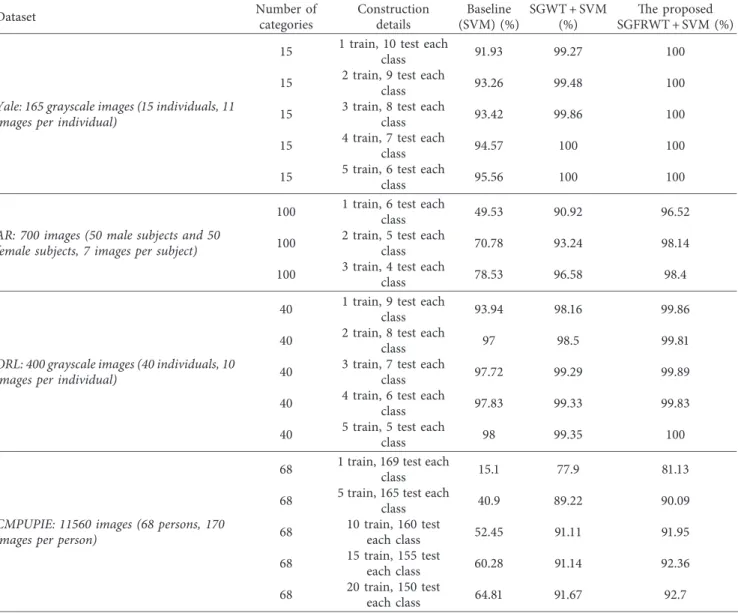
Table 3: The recognition results of the proposed SGFRWT feature, the SGWT feature, and the baseline on four face databases (Yale, AR, ORL, and CMU PIE). We randomly selected several images per individual as training set and the remaining images as testing set. “i train” means that we randomly choose i images in each class for training. The accuracy is the average results of ten random testing experiments.

Dataset Number of categories Construction details Baseline (SVM) (%) SGWT + SVM (%) The proposed SGFRWT + SVM (%)

Yale: 165 grayscale images (15 individuals, 11 images per individual)

15 1 train, 10 test each

class 91.93 99.27 100

15 2 train, 9 test each

class 93.26 99.48 100

15 3 train, 8 test each

class 93.42 99.86 100

15 4 train, 7 test each

class 94.57 100 100

15 5 train, 6 test each

class 95.56 100 100

AR: 700 images (50 male subjects and 50 female subjects, 7 images per subject)

100 1 train, 6 test each

class 49.53 90.92 96.52

100 2 train, 5 test each_class 70.78 93.24 98.14

100 3 train, 4 test each

class 78.53 96.58 98.4

ORL: 400 grayscale images (40 individuals, 10 images per individual)

40 1 train, 9 test each

class 93.94 98.16 99.86

40 2 train, 8 test each

class 97 98.5 99.81

40 3 train, 7 test each_class 97.72 99.29 99.89

40 4 train, 6 test each

class 97.83 99.33 99.83

40 5 train, 5 test each

class 98 99.35 100

CMPUPIE: 11560 images (68 persons, 170 images per person)

68 1 train, 169 test each

class 15.1 77.9 81.13

68 5 train, 165 test each

class 40.9 89.22 90.09

68 10 train, 160 test

each class 52.45 91.11 91.95

68 15 train, 155 test

each class 60.28 91.14 92.36

where the superscript T denotes transposition. C

denotes the number of classes. A is the mean of Ai

and Ai is the mean image of class Xiand Ni is the

number of images in class Xi.| X(θ, j)| denotes the

modulus of SGFRWT coefficient with the fractional order θ and the wavelet scale j.

(3) The SGFRWT features of three fractional orders are fused by canonical correlation analysis (CCA) [89] to obtain the feature vector, whose dimension is then reduced by principal component analysis (PCA) and Linear Discriminant Analysis (LDA). Finally, we feed the feature vector to the support vector machine (SVM). We conduct experiments on 18 different datasets which are constructed by four classical face databases mentioned above. Each set of datasets is compared with three different methods (baseline, SGWT, and SGFRWT), and we evaluate the classification accuracy on the testing set with an average value of 10 times. The recognition comparison results of the proposed SGFRWT feature building, the SGWT feature, and the baseline (only PCA + LDA + SVM used) on four face databases are shown in Table 3, from which we can see that the proposed SGFRWT feature building approach can achieve promising results and perform better than SGWT feature and also the SVM baseline.

6. Conclusion

This paper investigates the issue of extension of spectral graph wavelet transform (SGWT) to fractional domain. The main contributions of this paper can be summarized as follows. (1) A novel transform named spectral graph fractional wavelet transform (SGFRWT) is defined. (2) A Fourier series ap-proximation-based fast algorithm for SGFRWT is derived and implemented since the SGFRWT includes complex domain computations compared to SGWT. (3) Applications of SGFRWT to synthetic and real datasets are also given to highlight its potential usefulness. In summary, the proposed fractional spectral graph wavelets provide a new choice for the graph signal processing. Further research may include the extension of the proposed SGFRWT for dealing with the di-rected graphs [40, 41] and the extension of the idea of SGFRWT to critically sampled graph wavelets like GraphBio [46].

Appendix

A. Definition of SGFRWT by Using the Idea of

Traditional FRWT

According to (8), we can define the SGFRWT in (37) in another form by using the idea of traditional FRWT as follows: W_f(θ, s, n) � T􏼐 sg_θf􏼑(n) � 􏽘 N m�1 f(m)ψ∗_θ,s,n(m) �〈f, ψθ,s,n〉, n �1, . . . , N, (A.1) where Ts_g θ� e − j/2 m₍ 2_{− n}2_{− (m− n/s)}2_{)cot θ} g(sL), (A.2) ψθ,s,n(m) � e − j/2 m₍ 2_{− n}2_{− (m− n/s)}2₎ cot θ_􏽘 N−1 ℓ�0 g sλℓ􏼁χℓ(m)χ ∗ ℓ(n). (A.3)

From (A.3), we can see that this definition has two defects:

(1) The basis of SGFRWT ψθ,s,n(m) is still based on

χℓ(n); however, we want to define the basis of

SGFRWT ψθ,s,n(m) based on a new function, for

example, cℓ(n). If we use the definition of (A.3), then

the characteristic of ψθ,s,n(m)will be very similar to

ψs,n(m) in (22) since they are based on the same

function χℓ(n).

(2) We want to define the basis of SGFRWT ψθ,s,n(m)

which changes directly with λθℓ; that is, the parameter

θ should have an effect on λℓ directly.

Therefore, we do not use (A.1)–(A.3) to define the SGFRWT.

B. Definition of SGFRWT by Using Another

Graph Fractional Laplacian Operator L

Different from the definition in (24), the graph fractional Laplacian operator can also be defined as follows:

Lθ�􏼐χΛχH􏼑θ�χΛθχH. (B.1)

Comparing (B.1) and (13), we can see that the

decom-position of L and Lθshares the same χ. That is, if we define Lθ

as the graph fractional Laplacian operator, then, similar to (21), we can define the spectral graph fractional wavelet

transform (SGFRWT) operator Ts gθ as follows: W_f(θ, s, n) � T T􏼐 sg_θ, f􏼑(n) � 􏽘 N m�1 f(m)ψ∗_θ,s,n(m)〈f, ψθ,s,n〉, n �1, . . . , N, (B.2) where Ts_g θ� g sL θ 􏼐 􏼑, (B.3) ψθ,s,n(m) � 􏽘 N−1 ℓ�0 g s􏼐λθℓ􏼑χℓ(m)χ ∗ ℓ(n), m �1, 2, . . . , N. (B.4) From (B.4), we can see that this definition has one defect:

the basis of SGFRWT ψθ,s,n(m)is based on χℓ(n); however,

we want to define the basis of SGFRWT ψθ,s,n(m)based on a

new function, for example, cℓ(n). If we use the definition of

to ψs,n(m)in (21) since they are based on the same function

χℓ(n).

Therefore, we do not use (B.1)–(B.4) to define the SGFRWT.

C. Some Properties of SGFRWT

In this appendix, we give some properties of proposed SGFRWT without proof, since the proof of these properties is very similar to that of those properties of SGWT in [44].

Lemma C.1. If the SGFRWT kernel gθsatisfies the following

admissibility condition: 􏽚 ∞ 0 g2(x) x dx � Cg< ∞, (C.1) and g(0) � 0, then 1 C_g 􏽘 N n�1 􏽒 ∞ 0 W_f(θ, s, n)ψθ,s,n(m) ds s � f#(m), (C.2)

where f# � f − 〈c0,f〉c0. In particular, the complete

recon-struction is given by f � f# + 􏽢f(0)c0.

Lemma c.1 shows that the mean of f may not be re-covered from the zero-mean fractional graph wavelets. Lemma c.1 is a generalization of Lemma 5.1 in [44].

Lemma C.2. Let G be a weighted graph, Lθ the graph

fractional Laplacian operator, and t > 0 an integer. For any

two vertices m and n, if dG(m, n)> t then ((Lθ)

t₎

m,n�0.

Note that dG(m, n)is the shortest-path distance, i.e., the

minimum number of edges for any paths connecting m and

n. Lemma c.2 shows the localization result for integer powers

of the fractional Laplacian Lθ. Lemma c.2 is a generalization

of Lemma 5.2 in [44].

Lemma C.3. Let ψθ,s,n� Tsg_θδn and 􏽥ψθ,s,n� T_􏽥s_g

θδn be the

fractional wavelets at scale s generated by the fractional

kernels gθ and 􏽥gθ. If |g(sr) − 􏽥g(sr)|≤ M(s) for all

r∈ [0, rN−1], then |ψθ,s,n(m) − 􏽥ψθ,s,n(m)|≤ M(s) for each

vertex m. Additionally, ‖ψθ,s,n− 􏽥ψθ,s,n‖2≤

��

N

√

M(s).

Lemma c.3 shows that if two fractional kernels gθand 􏽥gθ

are close to each other in some sense, then the resulting graph fractional wavelets should be close to each other. Lemma 3.3 is a generalization of Lemma c.3 in [44].

Lemma C.4. Let gθ be K + 1 times continuously

differen-tiable, satisfying g(0) � 0, g(i)_{(0) � 0 for all i < K, and}

g(K)_{(0) � C ≠ 0. Assume that there is some s}

′

′

Lemma c.4 shows that if a fractional kernel gθhas a zero

of integer multiplicity at the origin, then gθ can be

approximated by a single monomial for small scales. Lemma c.4 is a generalization of Lemma 5.4 in [44].

Theorem C.1. Let G be a weighted graph with fractional

Laplacian Lθ. Let gθ be a kernel satisfying the hypothesis of

Lemma 3.4, with constants s′and B. Let m and n be vertices of

G such that dG(m, n)> K. Then, there exist constants D and

s″, such that ψθ,s,n(m)/‖ψθ,s,n‖≤ Ds for all s < min(s

_′

_″

Theorem c.1 shows that the localization of the fractional

wavelet ψθ,s,nmust include a renormalization factor in the limit

of small scales. In general, ψθ,s,n(m)⟶ 0 as s ⟶ 0 for all m

and n, due to the normalization chosen for the graph fractional wavelets. Theorem c.1 is a generalization of Theorem 5.5 in [44].

Theorem C.2. Given a set of scales 􏽮 􏽯s_j J_j�

1, the set F �􏽮ϕθ,n􏽯 N n�1∪ ψ􏼚 θ,sj,n􏼛 J j�1 N

n�1forms a frame with bounds A,

B given by A � minr∈[0,rN−1]G(r) and B � maxr∈[0,rN−1]G(r),

where G(r) � |h(r)|2+ 􏽐j|g(sjr)|2.

Note that the basic definition of a frame is as follows:

Given a Hilbert space H, a set of vectors Γk ∈ H form a

frame with frame bounds A and B if the inequality

A‖f‖2≤ 􏽐

k

|〈f,Γk〉|2≤ B‖f‖2holds for all f ∈ H. Theorem

C.6 shows that the numerical stability of recovering the

vector f from the inner product 〈f, Fk〉 depends on the

frame bounds A and B. Theorem c.2 is a generalization of Theorem 5.6 in [44].

Data Availability

The data used in Section 5.2.1 are synthetic graph data. The data used in Section 5.2.2 are MNIST dataset, which are downloaded from the homepage of Yann LeCun (http:// yann.lecun.com/exdb/mnist/). The data used in Section 5.2.3 are supported in [82, 83].

Conflicts of Interest

The authors declare that they have no conflicts of interest regarding the publication of this paper.

Acknowledgments

This work was supported in part by the National Natural Science Foundation of China under Grants 61876037, 31800825, 61871117, 61871124, and 61773117, in part by the National Science and Technology Major Project of the Ministry of Science and Technology of China under Grant 2018ZX10201002-003, in part by the Short-Term Recruitment Program of Foreign Experts under Grant WQ20163200398, and in part by INSERM under the Grant IAL.

References

[1] S. Mallat, A Wavelet Tour of Signal Processing: The Sparse Way, Academic Press, Cambridge, MA, USA, 3rd edition, 2008.