Interannual variability of global biomass burning emissions from 1997 to 2004

(1)

HAL Id: hal-00301203

https://hal.archives-ouvertes.fr/hal-00301203

Submitted on 18 Apr 2006

HAL is a multi-disciplinary open access

archive for the deposit and dissemination of sci-entific research documents, whether they are pub-lished or not. The documents may come from teaching and research institutions in France or abroad, or from public or private research centers.

L’archive ouverte pluridisciplinaire HAL, est destinée au dépôt et à la diffusion de documents scientifiques de niveau recherche, publiés ou non, émanant des établissements d’enseignement et de recherche français ou étrangers, des laboratoires publics ou privés.

Interannual variability of global biomass burning

emissions from 1997 to 2004

G. R. van der Werf, J. T. Randerson, L. Giglio, G. J. Collatz, P. S.

Kasibhatla, A. F. Arellano Jr.

To cite this version:

G. R. van der Werf, J. T. Randerson, L. Giglio, G. J. Collatz, P. S. Kasibhatla, et al.. Interannual variability of global biomass burning emissions from 1997 to 2004. Atmospheric Chemistry and Physics Discussions, European Geosciences Union, 2006, 6 (2), pp.3175-3226. �hal-00301203�

(2)

ACPD

6, 3175–3226, 2006

Interannual variability of global biomass burning emissions

G. R. van der Werf et al.

Title Page Abstract Introduction Conclusions References Tables Figures J I J I Back Close

Full Screen / Esc

Printer-friendly Version Interactive Discussion

EGU Atmos. Chem. Phys. Discuss., 6, 3175–3226, 2006

www.atmos-chem-phys-discuss.net/6/3175/2006/ © Author(s) 2006. This work is licensed

under a Creative Commons License.

Atmospheric Chemistry and Physics Discussions

Interannual variability of global biomass

burning emissions from 1997 to 2004

G. R. van der Werf1, J. T. Randerson2, L. Giglio3, G. J. Collatz4, P. S. Kasibhatla5, and A. F. Arellano Jr.5,*

1

Department of Hydrology and Geo-Environmental Sciences, Faculty of Earth and Life Sciences, Vrije Universiteit, Amsterdam, The Netherlands

2

Department of Earth System Science, University of California, Irvine, California, USA 3

Science Systems and Applications, Inc., NASA Goddard Space Flight Center, Greenbelt, Maryland, USA

4

NASA Goddard Space Flight Center, Greenbelt, Maryland, USA 5

Nicholas School of the Environment and Earth Sciences, Duke University, Durham, North Carolina, USA

*

now at: National Center for Atmospheric Research, Boulder, Colorado, USA

Received: 22 December 2005 – Accepted: 27 January 2006 – Published: 18 April 2006 Correspondence to: G. R. van der Werf (guido.van.der.werf@falw.vu.nl)

(3)

ACPD

6, 3175–3226, 2006

Full Screen / Esc

EGU

Abstract

Biomass burning represents an important source of atmospheric aerosols and green-house gases, yet little is known about its interannual variability or the underlying mech-anisms regulating this variability at continental to global scales. Here we investigated fire emissions during the 8 year period from 1997 to 2004 using satellite data and

5

the CASA biogeochemical model. Burned area from 2001–2004 was derived using newly available active fire and 500 m burned area datasets from MODIS following the approach described by Giglio et al. (2005). ATSR and VIRS satellite data were used to extend the burned area time series back in time through 1997. In our analysis we estimated fuel loads, including peatland fuels, and the net flux from terrestrial

ecosys-10

tems as the balance between net primary production (NPP), heterotrophic respiration (R_h), and biomass burning, using time varying inputs of precipitation (PPT), tempera-ture, solar radiation, and satellite-derived fractional absorbed photosynthetically active radiation (fAPAR). For the 1997–2004 period, we found that on average approximately 58 Pg C year−1 was fixed by plants, and approximately 95% of this was returned back

15

to the atmosphere via R_h. Another 4%, or 2.5 Pg C year−1 was emitted by biomass burning; the remainder consisted of losses from fuel wood collection and subsequent burning. At a global scale, burned area and total fire emissions were largely decoupled from year to year. Total carbon emissions tracked burning in forested areas (includ-ing deforestation fires in the tropics), whereas burned area was largely controlled by

20

savanna fires that responded to different environmental and human factors. Biomass burning emissions showed large interannual variability with a range of more than 1 Pg C year−1, with a maximum in 1998 (3.2 Pg C year−1) and a minimum in 2000 (2.0 Pg C year−1).

(4)

ACPD

6, 3175–3226, 2006

Full Screen / Esc

EGU

1 Introduction

The link between El Ni ˜no-Southern Oscillation (ENSO) and the CO₂growth rate vari-ability is well established (Bacastow, 1976; Keeling et al., 1995) and provides a test case scenario for the effects of future climate change under warm and dry conditions. During El Ni ˜no, drought in equatorial Asia and Central and South America

simultane-5

ously influences fire activity, net primary production (NPP) and heterotrophic respiration (R_h) in terrestrial ecosystems in a way that increases the growth rate of atmospheric CO₂. Although the link between drought and fire emissions is well established in high productivity ecosystems, its effect on the balance between NPP and R_hremains uncer-tain. In temperate ecosystems, for example, warm and dry conditions increased rates

10

of carbon uptake in a hardwood forest (Goulden et al., 1996), whereas a strong drought in Europe during the summer of 2003 led to carbon loss from multiple ecosystems (Ciais et al., 2005). In boreal regions, increased temperature may trigger increased soil thaw and a loss of soil carbon (Oechel et al., 1993; Goulden et al., 1998). In tropical regions, deep roots may enable trees to maintain high productivity during the

15

dry season, whereas the metabolic activity of surface soil microbes are simultaneously inhibited during these periods, lowering R_h and leading to a net carbon sink (Saleska et al., 2003). Longer-term time series of flux measurements from tropical ecosystems are sparse and limit our ability to assess the effect of drought on interannual to decadal timescales.

20

Several recent studies provide evidence that fires account for a substantial fraction of the variability in the CO₂growth rate (Langenfelds et al., 2002; Schimel and Baker, 2002; van der Werf et al., 2004), suggesting that variations in NPP and R_h are more closely coupled than previously thought. Observations from Indonesia show that fires in drained peatlands were a dominant source of emissions from this region during the

25

1997–1998 El Ni ˜no (Page et al., 2002). Interannual variability (IAV) in boreal fire activity is also large (Amiro et al., 2001; Sukhinin et al., 2004) and may be linked with the Arctic Oscillation and temperature anomalies (Balzter et al., 2005; Flannigan et al., 2005). At

(5)

ACPD

6, 3175–3226, 2006

Full Screen / Esc

EGU a global scale, two studies have assessed interannual variability in biomass burning

emissions using satellite data (Duncan et al., 2003; van der Werf et al., 2004). These biomass burning estimates are uncertain but are becoming better constrained, primar-ily from new satellite information on burned area, improved biogeochemical models used for estimating fuel loads, and atmospheric tracer inverse modeling studies.

As-5

suming that IAV in ocean-atmosphere exchange is relatively small as compared to that associated with the terrestrial biosphere (Lee et al., 1998; Battle et al., 2000; Bous-quet et al., 2000), reliable estimates of global biomass burning emissions may help to further constrain the climate sensitivity of processes within the terrestrial biosphere.

Fire emissions are commonly calculated as the product of burned area, fuel loads,

10

and combustion completeness, integrated over the time and space scale of interest. Burned area is usually considered to be the most uncertain parameter in emission estimates, and burned area estimates on a global scale have only recently become available. Both the GBA2000 (Gr ´egoire et al., 2002) and GLOBSCAR (Simon et al., 2004) efforts have yielded burned area estimates for the year 2000. The algorithms

15

used in both projects were recently combined to estimate burned area over a longer time series in the GLOBCARBON initiative (Plummer et al., 2006). Other approaches to estimate burned area on large scales rely on the detection of active fires (fire counts) and relationships between these fire counts and burned area (van der Werf et al., 2003; Giglio et al., 2005). More detailed information on burned area is available for

20

specific regions, and provides a basis for validating burned area algorithms developed at a global scale. Sukhinin et al. (2004) for example, estimated burned area for the 1995–2002 period for Russia using AVHRR data, and estimates of Canadian burned area from the Canadian Forest Service provide the longest time series of burned area available (http://fire.cfs.nrcan.gc.ca/research/climate change/lfdb e.htm). Fuel loads

25

are the next most uncertain parameter required for estimates of fire emissions. His-torically, biome-averaged values were used, but more recently satellite imagery has been used to represent heterogeneity within biomes (Scholes et al., 1996; Barbosa et al., 1999). Currently, most studies employ biogeochemical models to more accurately

(6)

ACPD

6, 3175–3226, 2006

Full Screen / Esc

EGU estimate fuel loads. This approach allows for a more direct comparison of aboveground

biomass levels estimated by the model with spatially explicit maps generated from re-mote sensing and field based studies (e.g., Houghton et al., 2001; Saatchi et al., 2001; Le Toan et al., 2004). Use of biogeochemical models also enables the incorporation of process-level information on herbivory and fuel wood collection that are important

5

controllers of fuel levels and will likely respond to global change processes and grow-ing populations over the next several decades. The Lund-Potsdam-Jena (LPJ) model has been used in several studies to estimate emissions, including estimating contem-porary emissions (Hoelzemann et al., 2004) and emissions during glacial-interglacial transitions (Thornicke et al., 2005). We previously implemented a fire module in the

10

Carnegie-Ames-Stanford-Approach (CASA) model to estimate contemporary patterns of tropical fire emissions (van der Werf et al., 2003), global variations in fire emissions over an ENSO cycle (van der Werf et al., 2004), and the effect of these variations on the atmospheric δ13CO₂ signature (Randerson et al., 2005). Regional-scale models have been employed to improve emissions predictions from boreal regions, including

15

the combustion of belowground fuels (Kasischke et al., 2005). Recent work indicates that the burning of belowground fuels may also be an important source of emissions in tropical regions (Page et al., 2002). Vast amounts of peat have been drained in Indone-sia and are vulnerable to fire during droughts, which happened during the 1997–1998 El Ni ˜no, releasing large quantities of carbon to the atmosphere (Page et al., 2002).

20

Only a fraction of the available fuel load is consumed during a fire event, and this fraction is represented within models by combustion completeness (CC). CC has been measured in the field for various biome and fuel types (e.g., Carvalho et al., 1995; Shea et al., 1996; Hoffa et al., 1999), and varies over the course of the fire season with more complete combustion at the end when fuels have had more time to dry out, as

25

shown by Hoffa et al. (1999) for savanna ecosystems. In general, fine and dry fuels burn more completely than coarse and wet fuels, although a paucity of data makes it challenging to quantitatively link CC with climate in global models. Although significant effort has been made to improve burned area and fuel estimates, uncertainties are still

(7)

ACPD

6, 3175–3226, 2006

Full Screen / Esc

EGU large and difficult to quantify, particularly in tropical forest biomes. Eliminating the need

for explicit knowledge of burned area, fuel loads, and CC, Wooster (2002) and Roberts et al. (2005) have shown for selected regions that satellite derived fire radiative energy can be used to directly estimate emissions, potentially providing an independent means to estimate emissions.

5

Although significant effort has been made to improve burned area and fuel esti-mates, uncertainties are still large and difficult to quantify, particularly in tropical forest biomes undergoing deforestation. New studies employing inverse modeling techniques combined with atmospheric measurements of trace gases allow for an independent estimate of biomass burning emissions, and progress has been made in identifying

10

deficiencies of current bottom-up estimates. To better constrain biomass burning esti-mates, comparisons against measurements of atmospheric CO proved especially use-ful since biomass burning is a major source of CO and is responsible for almost all of its temporal variability (Novelli et al., 2003; van der Werf et al., 2004). Arellano et al. (2004) used data from the Measurements Of Pollution In The Troposphere

(MO-15

PITT) sensor to demonstrate that inventories severely underestimated fossil fuel emis-sions from Asia, and identified several areas where our previous estimates of biomass burning emissions were inadequate. In a similar study that also examined seasonal patterns, P ´etron et al. (2004) demonstrated that MOPITT observations provided addi-tional constraints on the seasonal timing of fire emissions in the Southern Hemisphere,

20

especially in southern Africa.

Here we estimated biomass burning emissions on a global scale over the 1997–2004 period. We used the satellite-driven CASA biogeochemical model (Potter et al., 1993; Field et al., 1995; Randerson et al., 1996) that was previously modified to account for fires (van der Werf et al., 2003), in combination with a burned area time series derived

25

from the MODIS sensors (Giglio et al., 2005). We extended the burned area time series back in time before MODIS using data on fire activity from Arino et al. (1999) and Giglio et al. (2003). Our overall goal was to improve global biomass burning estimates, with specific objectives to better represent fuel loads in the boreal ecosystems and in

(8)

ACPD

6, 3175–3226, 2006

Full Screen / Esc

EGU wetlands by modeling the burning of soil organic carbon, to improve the seasonality of

emissions in regions where inverse studies indicated that inventories may misinterpret regional dynamics, and to analyze the relation between burned area and emissions on a global scale.

2 Methods

5

2.1 Burned area for the MODIS period (2001–2004)

In our analysis, we used the burned area data set developed by Giglio et al. (2005). For this product, burned area was mapped at 500×500 m spatial resolution within 52 globally-distributed MODIS tiles, with each tile covering an area of approximately 10◦×10◦, for different time periods between 2001 and 2004 (Giglio et al., 2005). MODIS

10

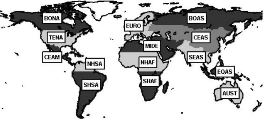
fire counts (Justice et al., 2002) were then calibrated with the 500-m burned area within 1◦×1◦ grid cells on a monthly basis, taking advantage of additional information about fire cluster size, fractional woody cover, herbaceous cover, or bare ground (Vegetation Continuous Fields, VCF – Hansen et al., 2003), and fire persistence. A unique regres-sion tree was grown for each region shown in Fig. 1. The set of regresregres-sion trees was

15

then used with the MODIS fire count time series to generate global monthly burned area estimates from January 2001 through December 2004. The selection of regions shown in Fig. 1 and Table 1 was based on similarities in fire behaviour and also on suitability for use as basis regions in atmospheric tracer inversion studies.

2.2 Burned area prior to the MODIS period

20

The Terra satellite that carried the first MODIS sensor was launched in December of 1999, but here we only used observations starting in January 2001 because of incon-sistent calibration during the first eight months of operation. To extend the time series back in time to January 1997, we used fire counts from the tropical rainfall measuring

(9)

ACPD

6, 3175–3226, 2006

Full Screen / Esc

EGU mission (TRMM) – visible and infrared scanner (VIRS) and European remote sensing

satellites (ERS) along track scanning radiometer (ATSR) sensors. VIRS observations are available for the TRMM footprint (38◦N–38◦S), starting in January 1998 (Giglio et al., 2003). ATSR observations are available globally, starting in July 1996 (Arino et al., 1999).

5

A comparison of the MODIS burned area time series with VIRS and ATSR obser-vations over the 2001–2003 period revealed two important differences between the datasets. The first was the difference in seasonality. In Southern Hemisphere tropi-cal ecosystems, and particularly in southern Africa, VIRS fire counts peak about two months earlier than ATSR and MODIS. Second, ATSR fire counts at the end of 2001

10

were anomalously low in northern Africa as compared to both VIRS and MODIS ob-servations. Because of these differences, in Africa we choose to use VIRS to set the IAV for the 1998–2000 period (and ATSR for 1997), while maintaining the seasonality as averaged over the 2001–2004 period from MODIS. For all other regions we used ATSR fire counts to set both the seasonal cycle and IAV.

15

The procedure used to convert VIRS or ATSR fire counts to burned area was based on an analysis of the 2001–2003 MODIS overlap period. For each grid cell the 2001– 2003 cumulative burned area for the three years derived from MODIS was divided by the cumulative VIRS/ATSR fire counts. The ratio represents the burned area per VIRS/ATSR fire count and was used to estimate burned area from VIRS/ATSR fire

20

counts before the MODIS era. In grid cells where no fire counts and burned area were observed in the MODIS era but fire counts were observed by VIRS/ATSR before the MODIS era, the weighted ratio MODIS burned area from neighbouring grid cells was used. We are aware that our approach to estimate burned area may introduce biases because of the use of different sensors, and ideally would like to use a consistent

25

satellite derived burned area time series. However, until high quality burned area data becomes available, we believe our approach may serve as an interim solution in the context of exploring interannual variations of biomass burning emissions.

(10)

ACPD

6, 3175–3226, 2006

Full Screen / Esc

EGU 2.3 Fuel loads

For each month and grid cell, fuel loads were calculated based on the fuel load of the previous month, input from NPP, and losses from R_h, fire, fuel wood collection, and herbivory. NPP was calculated using satellite based measurements of the Normalized Difference Vegetation Index (NDVI) from the Advanced Very High Resolution

Radiome-5

ter (AVHRR) data processed by the Global Inventory Modeling and Mapping Studies (GIMMS) lab, version “g” (Pinzon et al., 2006; Tucker et al., 2006). NDVI is converted to fraction absorbed photosynthetic active radiation (fAPAR, see below), and NPP was calculated as (Field et al., 1995):

NPP=fAPAR × PAR × ε_{(T ,P )} (1)

10

where PAR is Photosynthetic Active Radiation, and ε is the maximum light use e ffi-ciency (LUE) that is downscaled when temperature (T ) or moisture (P ) conditions are not optimal. See Table 2 for a summary of the different data sources that we used to drive CASA. We converted NDVI to fAPAR using techniques developed by Los et al. (2000). Monthly PAR was derived by adding anomalies from release 2 of the

Na-15

tional Centers for Environmental Prediction (NCEP) reanalysis data (Kanamitsu et al., 2002) to average monthly PAR from Bishop and Rossow (1991).

Interannually varying fAPAR was used to calculate NPP for grid cells receiving less than 1000 mm of mean annual PPT (MAP). Otherwise the monthly mean for the study period was used. This was done because for higher MAP regions (more productive,

20

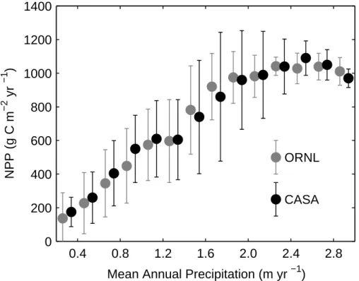
higher NPP) IAV was relatively low and may not exceed uncertainties in the NDVI ob-servations caused by residual signals from cloudiness and smoke. For all grid cells interannually varying PAR, T , and PPT were used to calculate monthly NPP. A compar-ison between CASA NPP estimates and results from the Oak Ridge National Labora-tory (ORNL) data base (Olson et al., 2001; Zheng et al., 2003) are shown as a function

25

of PPT in Fig. 2. At high PPT levels, CASA NPP levels off and may slightly decrease in a way that is consistent with observations. Mechanistically both nutrient limitation and light limitation have been proposed as limits on NPP in these mesic environments

(11)

ACPD

6, 3175–3226, 2006

Full Screen / Esc

EGU (Schuur, 2003), although with the version of CASA used in this study light limitation

was solely responsible for the model trend.

In CASA, NPP is distributed to live biomass pools (leaves, fine roots, and stems). Stems had a fixed turnover time depending on biome type. Leaf and fine root senesce depended on the seasonality of satellite derived Leaf Area Index (LAI), with the largest

5

transfer occurring when LAI declined (Randerson et al., 1996). Carbon from living pools was delivered to various litter pools that respire, both at the surface and in the soil. Each pool had a maximum turnover time assigned that was only reached when moisture and temperature were not limiting. The temperature sensitivity of R_h was based on a Q₁₀ value of 1.5. The moisture scalar used a simple bucket soil moisture scheme that was

10

a function of monthly PPT, T , and soil parameters including soil texture and moisture holding capacity. R_h was limited when soil moisture was low, but also saturated soils caused a decrease in R_hrates (Potter et al., 1993).

For each grid cell, we separately calculated the carbon exchange of herbaceous and of woody vegetation. NPP was allocated evenly to fine roots and leaves for herbaceous

15

vegetation, and evenly to fine roots, leaves, and stems for woody vegetation. The total grid cell carbon fluxes were then calculated from the proportional coverage of herbaceous and woody vegetation determined from the VCF. We estimated fuel wood collection and herbivory as in van der Werf et al. (2003). The main result of including these two processes was a decrease in fuel loads in savanna ecosystems, in better

20

agreement with measured fuel loads (Shea et al., 1996; Hoffa et al., 1999). Within tropical forest ecosystems, aboveground biomass levels from the model were broadly consistent with published estimates. For example, published estimates of aboveground biomass levels for the Brazilian Amazon range from 39 to 93 Pg C, with a mean of 70 Pg C and a standard deviation of 16 Pg C (Houghton et al., 2001). Here we estimated a

25

total of 77 Pg C using CASA for this same region. In the future, satellite or aircraft based estimates of vegetation height may enable a further reduction in uncertainties.

In the boreal region, a large fraction of the emissions comes from the combustion of soil organic carbon (SOC). Recent research in Indonesia has also highlighted the

(12)

ACPD

6, 3175–3226, 2006

Full Screen / Esc

EGU importance of SOC as fuel for combustion in tropical regions. The Indonesia case is

unique in that peat deposits have been systematically drained and thus have become vulnerable to fire during periods of drought (Page et al., 2002). Modeling SOC combus-tion is problematic because little informacombus-tion on depth of burning is available. Here we implemented a SOC parameterization that builds on the work of Ito and Penner (2004)

5

and Kasischke et al. (2005). SOC content values were taken from Batjes (1996), who analyzed over 4000 globally distributed soil profiles to estimate SOC at a 0.5◦×0.5◦ spatial resolution. In CASA, we adjusted the turnover times of the passive soil pools (the slow and armored soil pools that have relatively long turnover times) in each grid cell so that the CASA calculated SOC (both passive and active (or microbial) soil pools)

10

matched the measured SOC (Batjes, 1996). As a result, the largest adjustments to the turnover times were made in wetland areas, where anaerobic conditions lead to slow decay of carbon that was not taken into account in the model before. We used the natural wetland map of Matthews and Fung (1987) to distinguish between SOC that is accessible for fire and SOC associated with the mineral soil (and that does not burn).

15

In the boreal region, we considered the active soil and all surface litter pools as part of the duff layer, and these were always subject to a fire. In grid cells containing wetlands (both in the tropics and the boreal region), also carbon from the passive soil carbon pools could burn. In CASA, only the top 30 cm of the soil are considered within the model. To calculate what fraction of the passive soil carbon pool in CASA is lost

20

to fire, in the boreal region we used the “moderate severity” scenario of Kasischke et al. (2005) who suggested a maximum depth of 10 cm (average for surface and crown fires), or 33% of the CASA SOC, and for the tropical regions we set the maximum depth of burning to 30 cm, or 100% of CASA SOC. In the tropics, peat fires may burn even deeper than is possible within CASA. Page et al. (2002) for example, reported depth of

25

burning in Borneo during the 1997/1998 El Ni ˜no between 25 and 85 cm, with a mean of 51 cm. In CASA, the depth of burning in boreal regions was fully controlled by the soil moisture scalar and thus varied linearly between 0% (moist) and 33% (dry). In tropical regions the depth of burning and moisture conditions may be partly decoupled

(13)

ACPD

6, 3175–3226, 2006

Full Screen / Esc

EGU because of human influence of the fire processes. Therefore we assumed that fires in

tropical grid cells containing peat always burned 50% of the maximum depth (or 15 cm), the remainder being controlled by the moisture scalar as in boreal regions. Fires only burned to the maximum depth for some boreal grid cells at the end of the 1998, 2002, and 2003 fire season, and during the severe 1997/1998 El Ni ˜no in Indonesia.

5

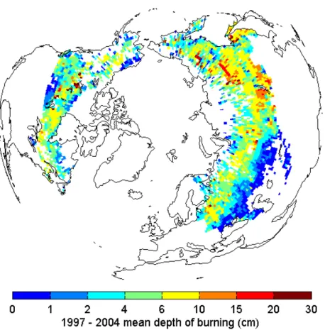
In our calculations, we assumed a constant SOC bulk density depending on the soil carbon content of the grid cell. In reality, the bulk density increases with depth due to compaction (Kasischke et al., 2005; Carrasco et al., 2006). By combining the calculated SOC carbon losses with the bulk density profile from Carrasco et al. (2006), we can calculate to which depth of burning our losses would correspond. The bulk

10

density profile of Carrasco et al. (2006) increases from approximately 0.015 g C cm−3 at the surface to approximately 0.020 g C cm−3 at 20 cm, and approximately 0.040 g C cm−3 at a depth of 40 cm. The corresponding depth of burning is shown in Fig. 3. Most of the forest fires burned to a depth of 4–10 cm. A few wetland areas had greater levels of fire severity, including fire complexes near Lake Baikal. Fires in grassland and

15

agricultural ecosystems south of the boreal forest consumed only a few centimetres or less.

2.4 Combustion completeness

The ratio of fire fuel consumption to total available fuels is known as the combustion completeness (CC) and is also referred to as the combustion factor. Several

general-20

ities about CC have emerged from studies that have measured CC’s in a wide range of vegetation types (e.g., Shea et al., 1996; Hoffa et al., 1999; Carvalho et al., 2001). First, CC of fine fuels is usually very high, up to 1 (complete combustion) for well aired and dry litter. Coarser fuels such as stems and woody debris, with a lower surface to area ratio, burn less completely. In boreal regions foliage and twigs have a high CC,

25

whereas living stems and boles have a low CC, in part because of their high water con-tent. Even though the boles remain largely intact, boreal fires across North America and parts of Siberia frequently induce stand-replacing mortality of the dominant conifer

(14)

ACPD

6, 3175–3226, 2006

Full Screen / Esc

EGU species. In contrast, in savannas fire-induced mortality of most large trees is quite

low because they are protected by a thick bark and because ground fuels often do not produce flames high enough to reach the foliage (Gill, 1981). CC in tropical forests undergoing deforestation is more challenging to characterize. Carvalho et al. (2001) reported an increase in CC with an increase in cleared area in deforestation regions in

5

the Brazilian state of Mato Grosso. Here, conversion is often highly mechanized and CC can approach unity over the course of a fire season as fuels including trunks are piled together and ignited multiple times (D. C. Morton and R. S. DeFries, personal communication).

The CASA model calculates different carbon pools (leaves, stems, fine roots, and

10

various litter pools), which allows CC to vary among fuel type, in contrast with earlier approaches where a single value was used for each biome. We allowed CC to vary from month to month as it is shown to increase when fuels have more time to dry out (Shea et al., 1996). We set minimum and maximum values for each fuel type (Table 3), and used moisture conditions to scale between these values. For live material (stems,

15

foliage), CC was scaled linear with the CASA NPP moisture scalar to simulate the CC dependence on the moisture content of the vegetation. CC of litter was scaled using the ratio of PPT over potential evaporation of the month of the fire and the previous month. To account for a longer memory of coarse fuels due to their greater volume to surface ratio the relative weighing of the previous and current month was 4:6 for coarse

20

woody debris and 1:9 for fine litter fuels.

To simulate higher CC due to repetitive burning in deforestation regions we increased the CC of stems and coarse litter in areas with high levels of fire persistence as identi-fied using the remote sensing approach described by Giglio et al. (2005). In these grid cells, the CC value was multiplied with a factor equal to the fire persistence, with an

25

(15)

ACPD

6, 3175–3226, 2006

Full Screen / Esc

EGU 2.5 Emission factors

Emission factors (EF) have been measured for multiple species in laboratories, ground based field studies, and from aircraft. EF’s are usually defined as grams of trace gas emitted per kg of dry matter (DM) consumed during the fire. Andreae and Merlet (2001) reviewed most of these studies and compiled EF’s for over 100 trace gas species.

5

EF’s were reported for different biomes and in general, the finer the fuel and thus the more efficient the fire, the higher the EF for CO₂ and the lower the EF for most other (reduced) trace gases. The fraction of emitted carbon that is CO₂ is usually referred to as combustion efficiency (CE). EF’s are not constant within biomes as shown by the relatively large standard deviation reported by Andreae and Merlet (2001). One reason

10

for variation within biomes may be the timing of fires; CE is usually lower in early season fires than in late season fires because fuels are drier later in the season. Korontzi et al. (2003) for example, showed how the EF for CO decreased from 100 to 40 g CO/kg DM in the first 6 weeks of a grassland fire season, while the CO₂EF increased from 1640 to 1770 g CO₂/kg DM during the same period, indicating an increase in

15

CE as the dry season progressed. On the other hand, woody vegetation may not be combustible until the end of the dry season, potentially decreasing the seasonal trend in EF. Because of this and because of limited information on the seasonal dependence of EF in other biomes, we have used the average values of Andreae and Merlet (2001) and Andreae (personal communication) in combination with the MODIS vegetation map

20

(MOD12C1 with the IGBP land cover classification, available online athttp://edcdaac. usgs.gov/modis/mod12c1v4.asp).

Emission factors for vegetation fires in Andreae and Merlet (2001) are reported for tropical forest, extratropical forest, and savanna and grassland. All grid cells in class 2 (evergreen broadleaf forest) were assigned the EF for tropical forest, all grid cells

25

in classes 1, 3, 4, and 5 (evergreen needleleaf forest, deciduous needleleaf forest, deciduous broadleaf forest, and mixed forest, respectively) were assigned the EF for extratropical forest, and other grid cells were assigned the EF for savanna and

(16)

grass-ACPD

6, 3175–3226, 2006

Full Screen / Esc

EGU land. In equatorial Asia, there were several savanna grid cells that had SOC burning,

because the Matthews and Fung (1987) maps indicated that these grid cells contained wetlands. For the combustion of the SOC in these grid cells, we used the EF from tropical forest instead of savanna to account for the lower CE. Most EF’s are reported for DM, we used a dry matter carbon content of 45% to convert carbon emissions to

5

DM burned.

3 Results and discussion

3.1 Global overview

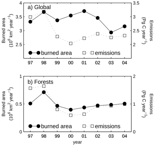
At a global scale, burned area and fire emissions were mostly decoupled over the 1997–2004 period (Fig. 4a). This was because most of the burned area occurred within

10

savanna ecosystems that had relatively low fuel loads and emissions. Burned area within forests biomes accounted for less than 20% of global burned area averaged over the 1997–2004 period. Nevertheless, burning in forests was highly variable from year to year and this variability, coupled with high fuel loads, meant that forests contributed to most of the variability in emissions (Fig. 4b). An exception occurred in 1997, when

15

burned area in forests was average but global emissions were high from fires in regions with tropical peatlands that have even higher fuel loads than forests (Table 5).

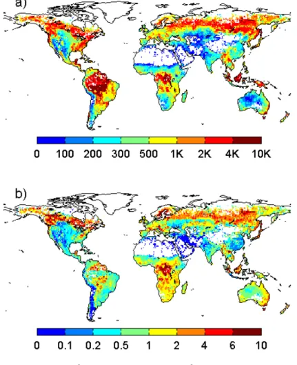
On average, emissions per unit burned area were 2.03 kg C m−2 in forest grid cells and 0.48 kg C m−2 in herbaceous grid cells (Fig. 5a). Emissions per fire count varied less between savanna and tropical forest biomes (Fig. 5b), suggesting that fire counts

20

may partly integrate the combined effects of burned area and fuel loads. There was still considerable variability in the amount of emissions per fire count across different regions, however, indicating that the relationship between fire counts and emission is not uniform.

Average emissions for the eight year study period were calculated to be 2460 Tg

25

(17)

ACPD

6, 3175–3226, 2006

Full Screen / Esc

EGU Andreae (personal communication) as described in Sect. 2.5 into 8903 Tg CO₂ yr−1,

433 Tg CO yr−1, and 21 Tg CH₄ yr−1 (Table 4). As a measure of IAV, the standard de-viation divided by the average (coefficient of variation, CV) was 0.16 for annual carbon emissions, 0.16 for CO₂, 0.21 for CO, and 0.27 for CH₄(Table 4). Because forest fires emit higher amounts of reduced species per unit carbon consumed, the relatively high

5

CV of CO and CH₄compared to CO₂is another indicator that IAV in emissions is largely driven by forest fires (Randerson et al., 2005). A map of mean annual emissions, aver-aged over the 1997–2004 period, is shown in Fig. 6. High levels of emissions occurred from well known biomass burning regions, including the boreal forests of North Amer-ica and Eurasia, tropAmer-ical AmerAmer-ica, AfrAmer-ica, Southeast Asia, and Australia. Fires were

10

present in all biomes except deserts.

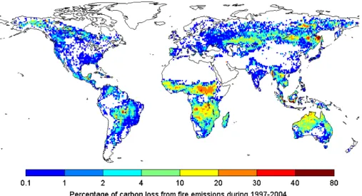
On a global scale, fire emissions accounted for 4.4% of the total carbon loss (R_h + fires) from terrestrial ecosystems during 1997–2004 (Fig. 7). This carbon was orig-inally fixed as NPP. The dominant loss pathway (not shown) was R_h. In frequently burning savanna grid cells, many of which are close to steady state over the study

15

period in our model, approximately 20% of total ecosystem carbon losses occurred via fire emissions. In some boreal regions that burned extensively and in tropical forests undergoing rapid clearing, and where fuels accumulated over many decades prior to our study interval, the percentage of fire loss was even higher.

3.2 Seasonal dynamics

20

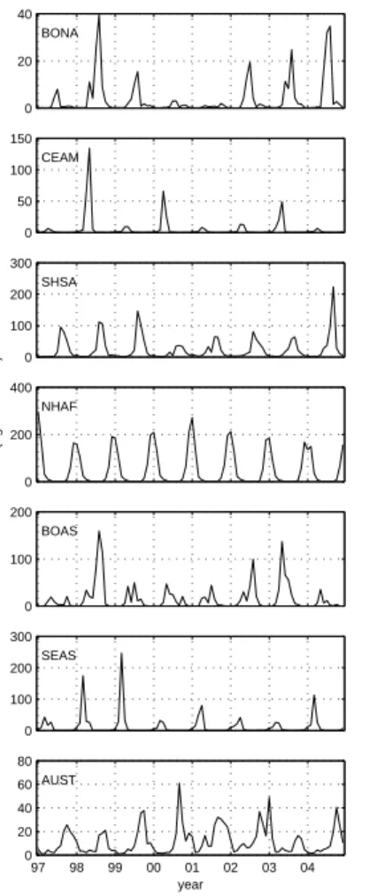
There was a clear distinction between the seasonality of fire emissions in boreal re-gions that usually burn during summer, and tropical rere-gions that burn during the hemi-sphere’s winter (Fig. 8). The burning season in the tropics was about 6 months out of phase with the annual movement of the Inter Tropical Convergence Zone (ITCZ). The seasonality of fire emissions in most regions was relatively constant throughout

25

our study period. There were a few exceptions. In boreal Asia, maximum levels of fire emissions in 2002 occurred in August, while in 2003 maximum fire emissions occurred

(18)

ACPD

6, 3175–3226, 2006

Full Screen / Esc

EGU in May. Other studies using ground and satellite based measurements of CO in the

northern hemisphere have previously noted the difference in seasonality between the two years (Edwards et al., 2004; Yurganov et al., 2005). Another region where the seasonality of emissions varied substantially was Central Asia; two peaks are visible in some years (1997, 2001, 2003) in Fig. 8, while in other years the first peak is less

5

pronounced (1998, 2002). In Equatorial Asia, only in 1998 after the strong El Ni ˜no, was substantial fire activity observed during February and March; usually the peak fire season happened later in the year during the August–October period.

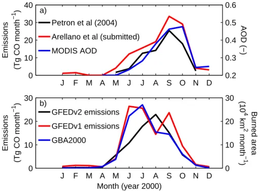
Studies using measurements of atmospheric CO from MOPITT have identified a substantial mismatch in seasonal timing of top-down (inverse) estimates of CO fluxes

10

vs. bottom-up biogeochemical model estimates (P ´etron et al., 2004; Arellano et al., 2006). In Fig. 9 we show results from Southern hemisphere Africa (SHAF) where the mismatch appeared largest. The MOPITT-derived approaches indicate that the peak fire season occurs in September; measurements of Aerosol Optical Depth (MOD08 M3, available online at http://modis-atmos.gsfc.nasa.gov/) indicate a peak

15

even a month later, in October (Fig. 9a). In contrast, both the GBA2000 burned area product and our previous emission estimates that were based on VIRS fire counts (GFEDv1; van der Werf et al., 2004) peaked in June or July, up to 4 months earlier (Fig. 9b). Even though the peak fire season shifts to August in our approach described here using MODIS fire counts, there is still a 1–2 month offset with respect to the

20

atmospheric-based approaches. There are several possible reasons for this continued offset. First, the fire season in SHAF shifts through time from west to east. When di-viding SHAF at longitude 25◦E, the fraction of total SHAF burned area that is observed west of 25◦E is 48% for GBA2000, 46% for GFEDv1, and 41% for the burned area used in this study (Giglio et al., 2005). Greater burned area and emissions in the west

25

causes the peak fire season for the entire region to advance to earlier times within the year. Another clue for the reasons behind this mismatch may come from aerosol characteristics; late season aerosols have a higher albedo than aerosols in the begin-ning of the season (T. Eck, personal communication), which is likely to be the result

(19)

ACPD

6, 3175–3226, 2006

Full Screen / Esc

EGU of more burning in woodlands than in grasslands. Woodland fires emit larger amounts

of CO per unit carbon burned than grassland fires, and this shift from grassland fires to woodland fires may not be captured by our coarse resolution modeling framework. Modeling at the MODIS native resolutions or even finer using other sensors may help in the future in identifying the role of these fine scale dynamics.

5

3.3 Burned area

The regions that burned most frequently during 1997–2004 were northern hemisphere Africa, southern hemisphere Africa, and Australia (Table 5). Together, these three savanna areas accounted for approximately 80% of global burned area during our study period. The total burned area derived in this study for all of Africa is 2.4 million

10

km2 year−1 in 2000, comparable to the 2.1 million km2 year−1 as calculated using another satellite based approach (GBA2000, Gr ´egoire et al. (2002)). The difference in total burned area in Australia, another region with mostly savanna and grassland fires, is somewhat larger: approximately 0.7 million km2as calculated here vs. approximately 0.5 million km2 by GBA2000. Detecting burned area in tropical deforestation areas

15

represents a greater challenge, both because of consistent cloud cover and because of human manipulation of fire processes. Detailed burned area estimates associated with deforestation cannot be given, because of great heterogeneity within the 1◦×1◦ grid cells we have used here, and because pasture fires within these grid cells will dominate the burned area numbers.

20

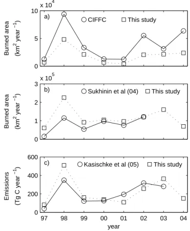
In boreal regions, our burned area time series was correlated with independent es-timates for Canada and Russia (Fig. 10), but the magnitude differed. Particularly in 1998 our results departed from other sources. For Canada, we found lower burned area than the Canadian Interagency Forest Fire Centre (CIFFC), and for Russia we found higher estimates than reported by Sukhinin et al. (2004). This may be a

conse-25

quence of the way we extended the MODIS burned area time series back in time using ATSR fire counts. Since ATSR only detects fires at night and fire activity peaks during daytime, ATSR may emphasize large fires that burn for longer periods, and thus also

(20)

ACPD

6, 3175–3226, 2006

Full Screen / Esc

EGU overemphasize anomalies. This is a potential reason for the higher burned area in the

high fire year of 1998 in boreal Asia than reported by Sukhinin et al. (2004). On the other hand, burned area estimates for Canada were lower than reported, but this was also the case during the MODIS years.

3.4 Fuel consumption

5

Combustion completeness (CC) and fuel loads were inversely related; in general the higher the fuel loads, the lower CC (Table 5). This was because high fuel loads were often a result of an increased fraction of stems and coarse woody debris in the fuel load, which had a low CC. Boreal regions and Equatorial Asia did not follow this trend; here SOC represented a large fraction of the fuel load (Table 5). In boreal regions,

10

biomass and litter pools were equally large, but a larger part of the emissions stemmed from the combustion of litter because of the higher CC observed for these fuels. CC was also high in deforestation regions (SHSA for example) because we increased CC for stems and coarse woody debris when there were high levels of fire persistence to represent repeated human aggregation and burning of fuels.

15

The highest fuel loads (over 11 kg C m−2) were predicted to occur in Equatorial Asia, because of high aboveground fuel loads and peats in wetland areas. Other tropical ar-eas where fires were being used to clear forests also had high fuel loads within burned areas, including Central and South America. In both boreal North America and bo-real Asia, fuel loads were approximately 3.5 kg m−2, and were separated almost evenly

20

between aboveground biomass and litter fuels. In savanna regions, fuel loads were highest in southern hemisphere Africa (1.3 kg m−2) because a substantial part of the burning occurred in woodland areas, and were lowest in Australia (0.4 kg m−2) where much of the burning occurred in low productivity grasslands. Fuel loads in northern hemisphere Africa fell in between these two regions, with approximately 0.7 kg m−2.

25

In frequently burning savannas, there was a clear upper threshold value on fuel consumption. Most savannas that burned annually were the more productive savannas with NPP values of approximately 1000 g C m−2 year−1 (van der Werf et al., 2003).

(21)

ACPD

6, 3175–3226, 2006

Full Screen / Esc

EGU Since half of the NPP was allocated belowground and was not accessible for fires, fuel

loads in annual burning savannas were at most 500 g C m−2. However, not all above ground biomass was available for fires since microbes, herbivores, and humans also compete for the available carbon. In addition to this upper threshold, there was also a lower threshold of approximately 100 g C m−2 that may represent the minimum levels

5

of fuel necessary to sustain fire spread (van Wilgen and Scholes, 1997). We found that the majority of the fires in Africa consumed between 200 and 400 g C m−2 year−1 (Fig. 11a), which is on the high end of most remote sensing and modeling studies (Scholes et al., 1996; Barbosa et al., 1999; H ´ely et al., 2003).

In tropical America (CEAM, NHSA, SHSA) there was a clear distinction between

10

pasture maintenance and savanna fires that accounted for much of the burned area but consumed little fuel, and deforestation fires with much larger fuel consumption but lower burned area (Fig. 11b). Pasture maintenance fires occur in managed grasslands and are ignited on purpose, mainly to prevent trees from invading the landscape and for nutrient recycling. In Africa, there were fewer fires with high fuel consumption (>3 kg C

15

m−2 year−1), providing evidence for less fire-driven deforestation than in South Amer-ica. Fuel consumption in the boreal regions was for a large part driven by soil carbon (Table 5). In boreal North America, the majority of the fires consumed between 1 and 2.5 kg C m−2year−1, stemming largely from combustion of the duff layer and SOC, and with minor contributions from stems and leaves (Fig. 11c). This distribution is similar to

20

the measured distribution reported by Amiro et al. (2001) 3.5 Emissions

Average annual emissions over the 8 year time period were 2.5 Pg C year−1(Tables 4 and 6, Fig. 12b). African emissions accounted for 49% of the total and southern hemi-sphere South America contributed another 12%. Other major contributors included

25

Equatorial Asia (11%), boreal regions (9%), Southeast Asia (6%), and Australia (6%). Over the 8 year period, there was significant IAV, especially during the first 4 years (Fig. 12b). Emissions in both 1997 and 1998 were approximately 1 Pg C year−1higher

(22)

ACPD

6, 3175–3226, 2006

Full Screen / Esc

EGU than in 2000, when global PPT was at a maximum (Adler et al., 2003, Fig. 12a). 1997

was a high fire year because of emissions in equatorial Asia, largely stemming from the combustion of peat in Indonesia (Page et al., 2002). 1998 was a high fire year because of increased burning across multiple continents, including equatorial Asia, boreal North America and Asia, and Central America. Only in northern hemisphere

5

Africa and Australia were emissions below average (Table 6). During the final 4 years of the study period, the range of emissions was lower, but emissions were elevated from 2000.

By far the region with the largest IAV was equatorial Asia, both in absolute and in relative terms, with a standard deviation that was approximately 1.3 times larger than

10

the average (Table 6). Emissions in 1997 were over 20 times as high as emissions in the year 2000, indicating a strong dependence on local climate and/or human activ-ity. Emissions in equatorial Asia were elevated again in 2002. More detailed inversion studies using MOPITT should further constrain the magnitude of these 2002 anoma-lies, and their impact on high CO₂growth rates at that time. Other regions with

substan-15

tial IAV include boreal America and Asia, Central America, and northern hemisphere South America. IAV in frequently burning Africa was low.

Most of the savanna and grassland fires occurred in Africa and Australia. Aver-age annual emissions from Africa were 1203 Tg C year−1, and emissions from north-ern hemisphere Africa (627 Tg C year−1) were somewhat higher than emissions from

20

southern hemisphere Africa (576 Tg C year−1). Average fuel consumption on the other hand, was higher in southern hemisphere Africa largely because relatively more fires were detected in woodlands, whereas almost all the fires in northern hemisphere Africa occurred in grasslands with lower percentages of woody vegetation. IAV was relatively low in Africa, with a CV of only 9%. Other studies have reported lower emissions

(Sc-25

holes et al., 1996; Barbosa et al., 1999; Hoelzemann et al., 2004), but relatively higher IAV (Barbosa et al., 1999). Most of this difference can probably be attributed to higher fuel loads in our study as our burned area estimates are comparable or even lower than those reported in previous studies. Only emissions calculated by Ito and Penner

(23)

ACPD

6, 3175–3226, 2006

Full Screen / Esc

EGU (2004) are comparable to our estimates, with a difference of about 10%, depending on

the scenario used by Ito and Penner (2004). 3.6 Net biome productivity

Average annual NPP was 58 Pg C year−1. Annual NPP and R_h values were approx-imately 23 times larger than fire fluxes (58 vs. 2.5 Pg C year−1). As a consequence,

5

relatively small variations in the balance between NPP and R_h can have a large effect on IAV of net biome productivity (NBP) and the CO₂ growth rate. NPP was highest in 2000 and lowest in 1998, with a difference of 1.8 Pg C yr−1 (Fig. 12). About 95% of NPP was returned to the atmosphere via R_h. Variability of R_h between years was similar to NPP, but with a smaller amplitude. The highest levels of R_hwere observed in

10

2000, and lowest in 1998 and 2002, with a difference of approximately 1.0 Pg C yr−1. Because NPP and R_htended to vary in parallel in CASA, the net ecosystem produc-tion (NEP, NPP–R_h) signal was smaller than the NPP signal. The largest net uptake occurred in 2000 and 2002, while most carbon was released during 1998 because NPP was inhibited more than R_h. In 2003 variations in NPP and R_h were somewhat di

ffer-15

ent from other years; the drop in R_h was approximately the same as the drop in NPP (Fig. 12b–c). The NEP signal was amplified by IAV in fires. The net result was that net biome production (NBP=NEP–fires) had a larger amplitude than NEP. This was most evident during the first 4 years of the study period.

3.7 Differences with earlier estimates

20

Emission estimates from our earlier studies were released in 2004 as the “Global Fire Emissions Database” (GFED version 1), covering the 1997–2001 period. These esti-mates were compared to results from, or used as a priori information in, several inver-sion studies (Arellano et al., 2004; P ´etron et al., 2004; van der Werf et al., 2004). The main limitations of GFEDv1 as indicated by inversion studies were the

underestima-25

(24)

ACPD

6, 3175–3226, 2006

Full Screen / Esc

EGU and in the boreal regions. Inversion analyses suggest that GFEDv1 overestimated the

magnitude of southern Africa emissions and that the seasonal phasing of emission in this region was off by several months.

Discrepancies between the inversion studies and our bottom-up results may help to identify regions where the bottom-up approach has a problem representing biomass

5

burning processes, assuming that the emission factors that translate the carbon emis-sions into the CO fluxes used in these inveremis-sions are correct (and that the inversion doesn’t suffer from other types of biases). One example is the combustion of peat that was not taken into account in GFEDv1, and may have been partly responsible for the underestimation of emissions from equatorial Asia.

10

There are numerous differences between the results presented here and those pre-viously reported in GFEDv1, mainly stemming from the use of improved burned area and the inclusion of SOC burning. For GFEDv1 we used a single global relationship between fire counts, fraction tree cover, and burned area. Here, many more MODIS scenes with burned area were available for fire count calibration, allowing us to use

15

regionally-based fire count to burned area relationships that depended on fire count cluster size and fire persistence, in addition to fractional tree cover (Giglio et al., 2005). This has led to a decrease of Southern African emissions because of lower burned area. The inclusion of SOC burning increased emissions in the boreal region and equatorial Asia. Another improvement occurred in deforestation regions in the Amazon

20

and in Indonesia. We formerly had a broad band of relatively low emissions around the main deforestation areas, our new results indicate that the emissions are higher in a smaller band known to have high rates of clearing (e.g., Mato Grosso, south and east Kalimantan). However, total emissions in Central and Southern America are lower in our current inventory, and diverge from results obtained from inverse studies (that

25

(25)

ACPD

6, 3175–3226, 2006

Full Screen / Esc

EGU 3.8 Uncertainties

3.8.1 Burned area

Burned area estimates have only recently become available from different satellite sen-sors, allowing for a comparison of different approaches. In boreal and tropical savanna ecosystems, independent estimates of burned area are converging, for large regions

5

within 20%, although from year to year the differences can be larger. Obviously this does not rule out as the possibility that independent products can suffer from identical biases, but it does provide some optimism compared to earlier estimates that differed over a factor 2 (Kasischke and Penner, 2004).

In deforestation regions, burned area estimates remain poorly constrained. There

10

are several reasons for this, the most important being consistent cloud cover and mechanized clumping of fuels that make burned area detection more problematic. The approach of Giglio et al. (2005) detects more burned area in areas undergoing active deforestation than other published estimates (Gr ´egoire et al., 2002; Simon et al., 2004), but it remains unclear how to assess uncertainty levels associated with this product.

15

With greater use of high resolution satellite data it the future, it is likely that burned area estimates will increase, especially in closed-canopy tropical forest ecosystems (Silva et al., 2005).

Because we used a statistical approach to estimate burned area from fire counts (Giglio et al., 2005), burned area estimates were available only for coarse resolution

20

grid cells. This may introduce a bias when fire processes show spatial heterogeneity. Future studies of global biomass burning emissions will profit from comparisons with studies that used burned area at finer resolution, ideally employing methods to scale up from high to coarse resolutions.

(26)

ACPD

6, 3175–3226, 2006

Full Screen / Esc

EGU 3.8.2 Fuel loads

As burned area estimates improve from higher resolution satellite data and refined algorithms, uncertainties in fuel loads may become the limiting factor in estimating emissions. Although using satellite data has improved spatial and temporal variabil-ity in fuel loads, approaches for calibrating these estimates using measured values

5

are still in their infancy. Reasons for this include a mismatch in scale between the measurements at plot level and the much coarser model grid cell, and a lack of data. Therefore, calibrating against satellite based measurements of, for example, biomass estimates based on satellite measured vegetation height is a necessary step for de-creasing uncertainties. Following Amiro et al. (2001) and H ´ely et al. (2003), we have

10

presented a histogram of carbon consumption (Fig. 11). These histograms provide an efficient means to directly compare carbon consumption between models and with field measurements.

3.8.3 Emissions

At a global scale, perhaps the strongest constraints on total emission from fires come

15

from inversion studies that take advantage of CO measurements. Using MOPITT ob-servations, an atmospheric model, and emission factors from Andreae and Merlet (2001), Arellano et al. (2006) estimated that global fire emissions for the April 2000 through March 2001 period were 3.4±1.0 Pg C year−1. This global estimate is consid-erably higher than several recent bottom-up emission estimates. For example,

Hoelze-20

mann et al. (2004) estimated emissions for the year 2000 to be 1.7 Pg C year−1, while Ito and Penner (2004) estimate was 1.3 Pg C year−1, also for 2000. In the same year, our estimate was 2.0 Pg C year−1. Clearly, uncertainties in bottom-up estimates are still very high, and likely underestimate actual emissions.

(27)

ACPD

6, 3175–3226, 2006

Full Screen / Esc

EGU

4 Conclusions

We have provided new constraints on biomass burning emissions over the 1997–2004 period, using improved satellite derived information on seasonality and extent of burn-ing, and a more complete fuel load parameterization. The main conclusions from this study can be summarized as follows:

5

1. Average annual biomass burning emissions as calculated by our model were 2.5 Pg C year−1 over the 1997–2004 period. The dominant contributors were Africa (49%), South America (13%), equatorial Asia (11%), boreal regions (9%), and Aus-tralia (6%).

2. Interannual variability over the 8 year period was large, especially in the first

10

4 years. Emissions in the years 1997 and 1998 were approximately 1 Pg C year−1 higher than emissions in 2000, following the ENSO pattern. 1997 was large because of the combustion of peat in equatorial Asia, 1998 was large because almost all major biomass burning regions showed increased emissions. Largest interannual variability was observed in equatorial Asia with a standard deviation that was 1.3 times as large

15

as the average, while interannual variability in Africa was relatively low, with a standard deviation of only 0.1 times the average.

3. Annual burned area and fire emissions were largely decoupled at a global scale over the 1997–2004 period because of differences in fuel loads between forests and grasslands. On a global scale, burned area was dominated by savannas, but

interan-20

nual variability of burned area was relatively larger in forested ecosystems. This IAV with the much higher fuel loads in forests was responsible for most of the interannual variability in global emissions.

4. The seasonality of our estimates more closely matched the seasonality derived from atmospheric measurements of CO and aerosols than our previous estimates and

25

other bottom-up estimates. However, there is still a mismatch of 1–2 months in south-ern hemisphere Africa. A potential reason for this could be a shift from grassland fires early in the dry season to woodland fires later in the dry season, a pattern that may not

(28)

ACPD

6, 3175–3226, 2006

Full Screen / Esc

EGU be captured by our course resolution modeling framework.

5. Uncertainties in biomass burning estimates are highest in deforestation regions and in regions where peat fires occur. Although the numbers presented in this study are thought to be a clear step forward from earlier estimates, inversion methods are needed to further refine these estimates. In this respect, multi-species inversions may

5

be particularly effective in lowering systematic errors stemming from biases in emis-sions factors. Especially in deforestation regions and in other regions where spatial heterogeneity is large, finer resolution bottom-up modeling also has the potential to substantially reduce uncertainties.

6. Variations in global NPP and R_h followed variations in global precipitation, with

10

high increased NPP and R_h during wet spells and vice versa. Since the amplitude of NPP variations exceeded R_h, drought years resulted in a CO₂ source. This was most evident during the first 5 years of the study period. This effect amplified the signal to the atmosphere from biomass burning (or vice versa).

Acknowledgements. We thank J. E. Pinzon and M. E. Brown from NASA Goddard’s Global

15

Inventory Modeling and Mapping Studies (GIMMS) for providing the NDVI time series, and E. S. Kasischke for helpful discussion about biomass burning in boreal regions. This work was supported by NASA grant NNG04GK49G to J. T. Randerson and NASA grant NNG04GD89G to P. S. Kasibhatla. G. R. van der Werf is supported by CarboEurope and the Laboratoire des Sciences du Climat et l’Environnement (LSCE), Gif sur Yvette, France.

20

The emission estimates presented here (carbon and several trace gas and aerosol species), as well as burned area, fuel loads, and combustion completeness values can be downloaded fromhttp://ess1.ess.uci.edu/\%7Ejranders/data/GFED2/.

References

Adler, R. F., Huffman, G. J., Chang, A., Ferraro, R., Xie, P. P., Janowiak, J., Rudolf, B.,

25

Schneider, U., Curtis, S., Bolvin, D., Gruber, A., Susskind, J., Arkin, P., and Nelkin, E.: The version-2 global precipitation climatology project (GPCP) monthly precipitation analysis (1979–present), J. Hydrometeorol., 4, 1147–1167, 2003.

(29)

ACPD

6, 3175–3226, 2006

Full Screen / Esc

EGU

Amiro, B. D., Todd, J. B., Wotton, B. M., Logan, K. A., Flannigan, M. D., Stocks, B. J., Mason, J. A., Martell, D. L., and Hirsch, K. G.: Direct carbon emissions from Canadian forest fires, 1959-1999, Canadian J. Forest Res., 31, 512–525, 2001.

Andreae, M. O. and Merlet, P.: Emission of trace gases and aerosols from biomass burning, Global Biogeochem. Cycles, 15, 955–966, 2001.

5

Arellano, A. F., Kasibhatla, P. S., Giglio, L., van der Werf, G. R., and Randerson, J. T.: Top-down estimates of global CO sources using MOPITT measurements, Geophys. Res. Lett., 31, doi:10.1029/2003GL018609, 2004.

Arellano, A. F., Kasibhatla, P. S., Giglio, L., van der Werf, G. R., Randerson, J. T., and Collatz, G. J.: Time-dependent inversion estimates of global biomass burning CO emissions using

10

MOPITT measurements, J. Geophys. Res., accepted, 2006.

Arino, O., Rosaz, J.-M., and Goloub, P.: The ATSR World Fire Atlas. A synergy with ‘Polder’ aerosol products, Earth Obs. Quarterly, 1–6, 1999.

Bacastow, R. B.: Modulation of Atmospheric Carbon-Dioxide by Southern Oscillation, Nature, 261, 116–118, 1976.

15

Balzter, H., Gerard, F. F., George, C. T., Rowland, C. S., Jupp, T. E., McCallum, I., Shvidenko, A., Nilsson, S., Sukhinin, A., Onuchin, A., and Schmullius, C.: Impact of the Arctic Oscilla-tion pattern on interannual forest fire variability in Central Siberia, Geophys. Res. Lett., 32, doi:10.1029/2005GL022526, 2005.

Barbosa, P. M., Stroppiana, D., Gregoire, J. M., and Pereira, J. M. C.: An assessment of

vegeta-20

tion fire in Africa (1981–1991): Burned areas, burned biomass, and atmospheric emissions, Global Biogeochem. Cycles , 13, 933–950, 1999.

Batjes, N. H.: Total carbon and nitrogen in the soils of the world, Eur. J. of Soil Sci., 47, 151– 163, 1996.

Battle, M., Bender, M. L., Tans, P. P., White, J. W. C., Ellis, J. T., Conway, T., and Francey, R.

25

J.: Global carbon sinks and their variability inferred from atmospheric O-2 and delta C-13, Science, 287, 2467–2470, 2000.

Bishop, J. K. B. and Rossow, W. B.: Spatial and temporal variability of global surface solar irradiance, J. Geophys. Res.-Oceans, 96, 16 839–16 858, 1991.

Bousquet, P., Peylin, P., Ciais, P., Le Quere, C., Friedlingstein, P., and Tans, P. P.: Regional

30

changes in carbon dioxide fluxes of land and oceans since 1980, Science, 290, 1342–1346, 2000.