HAL Id: hal-01997336
https://hal.archives-ouvertes.fr/hal-01997336
Submitted on 28 Jan 2019HAL is a multi-disciplinary open access
archive for the deposit and dissemination of sci-entific research documents, whether they are pub-lished or not. The documents may come from teaching and research institutions in France or abroad, or from public or private research centers.
L’archive ouverte pluridisciplinaire HAL, est destinée au dépôt et à la diffusion de documents scientifiques de niveau recherche, publiés ou non, émanant des établissements d’enseignement et de recherche français ou étrangers, des laboratoires publics ou privés.
UNIF: a Simulation Framework for Numerical
Integration Models
Bruno Bachelet, Jean-François Soussana, Stéphane Witzmann
To cite this version:
Bruno Bachelet, Jean-François Soussana, Stéphane Witzmann. UNIF: a Simulation Framework for Numerical Integration Models. [Research Report] FGEP/RR06-10, Unité de Recherche en Agronomie, INRA. 2006. �hal-01997336�
Bruno Bachelet1and Jean-François Soussana2
Agronomy Research Unit, INRA
234, Avenue du Brézet, 63100 Clermont-Ferrand, France. Stéphane Witzmann3
ISIMA, Université Blaise-Pascal
Campus des Cézeaux, BP 10125, 63173 Aubière, France. Research Report FGEP/RR06-10
October 31, 2006
Abstract
This paper presents a simulation framework called UNIF (Unified Numerical Integration
Frame-work) to design numerical integration models, i.e. models mainly ruled by ordinary differential
equations. We describe the object-oriented structure of UNIF, which allows to model a system as a hierarchical aggregation of subsystems interacting together, each one having a set of inputs, out-puts and integration variables that are involved in a set of equations. The use and the advantages of this framework are illustrated on a full biological model, called GEMINI (Grassland Ecosystem
Model with INdividual-centered Interactions), that simulates the life of populations of grassland
plants competing for light and soil resources.
Keywords: simulation, modeling, numerical integration, object-oriented framework.
Résumé
Cet article présente un cadriciel de simulation appelé UNIF (Unified Numerical Integration
Fra-mework) pour concevoir des modèles à intégration numérique, i.e. des modèles principalement
gouvernés par des équations différentielles ordinaires. Nous décrivons la structure orientée ob-jet d’UNIF, qui permet de modéliser un système comme une agrégation hiérarchique de sous-systèmes interagissant entre eux, chacun ayant un ensemble d’entrées, de sorties et de variables d’intégration qui sont impliquées dans un ensemble d’équations. L’utilisation et les avantages de ce cadriciel sont illustrés sur un modèle biologique complet, appelé GEMINI (Grassland
Ecosys-tem Model with INdividual-centered Interactions), qui simule la vie de populations de plantes de
prairie en compétition pour des ressources de lumière et du sol.
Abstract
This paper presents a simulation framework called UNIF (Unified Numerical Integration
Framework) to design numerical integration models, i.e. models mainly ruled by ordinary
differential equations. We describe the object-oriented structure of UNIF, which allows to model a system as a hierarchical aggregation of subsystems interacting together, each one having a set of inputs, outputs and integration variables that are involved in a set of equations. The use and the advantages of this framework are illustrated on a full biological model, called GEMINI (Grassland Ecosystem Model with INdividual-centered Interactions), that simulates the life of populations of grassland plants competing for light and soil resources.
keywords: simulation, modeling, numerical integration, object-oriented framework.
Introduction
The UNIF framework (Unified Numerical Integration Framework) presented in this paper pro-poses a generic structure to design and simulate numerical models. More precisely, we consider here models that can be expressed as sets of ordinary differential equations [2]. In this paper, we call such models numerical integration models.
Many tools exist to design this kind of models: Simulink-MATLAB, ACSL Sim, Simscript... However they seldom propose an object-oriented approach, which is necessary when developing huge models such as GEMINI (Grassland Ecosystem Model with INdividual-centered
Interac-tions) that will be used here to illustrate the functionalities of the UNIF framework.
Object-orientation allows to provide a flexible structure that eases the specialization of models, the acti-vation / deactiacti-vation of submodels, the coupling of models...
The UNIF framework is based on a fully object-oriented structure. It has been developed with the C++ language since 2004, and allows to design a model ruled by ordinary differential equations using the classical relationships of the object-oriented paradigm (mainly inheritance and composition).
Moreover, it is difficult to model a large system with differential equations only, as proposed in many tools, and it may be necessary to express some aspects of the system with discrete events. The UNIF framework is able to deal with these discrete events, while centered on continuous simulation: events can be triggered before and after each integration step.
Some classical functionalities of numerical integration tools are still necessary, such as a con-trol on the variables of a model (e.g. negativity or divergence check), and the possibility to change the integration method (Euler, Runge-Kutta... [7]) to simulate the evolution of a system ruled by ordinary differential equations.
Section 1 presents an overview of the structure of the UNIF framework. Section 2 briefly introduces the GEMINI model, which will be used all along the paper to illustrate the functional-ities of the framework. This is a model that simulates the life of populations of grassland plants competing for light and soil resources. Section 3 shows how to design a single model, i.e. without submodels. The specific structure of a model in the UNIF framework can thus be presented, and the simulation process can be described. Section 4 explains how to design a complex model, i.e. with submodels interacting together. A more precise view of the simulation process can thus be described. Section 5 presents briefly the graphical user interface of the UNIF framework. Finally, a conclusion summarizes the advantages of the UNIF framework from our GEMINI experience, and also presents some drawbacks and issues that must be addressed in a near future.
2
1
Overview of the UNIF Framework
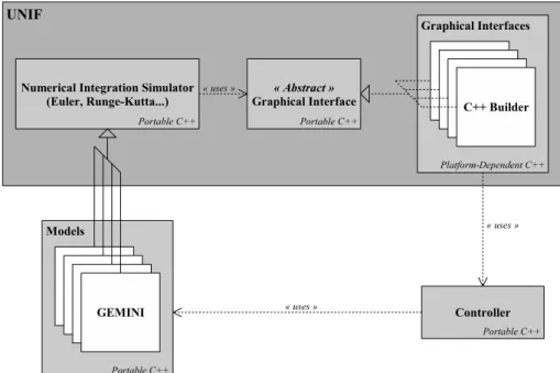
The UNIF framework provides a generic object-oriented platform written in C++. The core pack-age, the numerical integration simulator, is a set of classes that can be extended to develop new models. It is possible to design visual simulation through a set of abstract classes that represents the graphical interface of the application (Figure 1). Several implementations of this graphical interface can be provided, but only a Windows interface has been developed yet, with the Borland C++ Builder environment.
Figure 1: Structure of the UNIF framework.
The graphical interface can also integrate a user interface, i.e. a model can be parameterized, simulated and analyzed through this interface. For this purpose, an intermediate component called
controller has been designed to handle the models. Only those registered to this controller can be
managed by a user interface.
This structure of the UNIF platform makes the simulator package and the models independent of any graphical user interface. They have been designed to be fully portable and have been tested yet on several platforms: Borland C++ Builder (Windows) and GCC compilers (Cygwin, Linux...). A command-line user interface has also been developed in order to deploy a simulation experiment on a cluster or a grid.
2
The GEMINI Model
The GEMINI model aims at representing the life of populations of grassland plants that compete for light and soil resources, under external actions related to human activity like fertilizing, grazing of animals, cutting... GEMINI is the coupling of previous models: Soilopt and Canopt, both developed by the Grassland Ecosystem Research team (FGEP) of the INRA French institute.
Soilopt has been developed since 1998. It models a soil and its microbial population with compartments (9 organic and 3 mineral ones). These compartments represent amounts of vari-ous matters in the soil. The fluxes of carbon and nitrogen exchanged between the compartments
Research Report FGEP/RR06-10
are ruled by differential equations [6]. More recently, this model considers the priming effect: fresh organic matter resulting from plant death allows microbes to get more energy, and thus, to decompose the organic matter inside the soil [3].
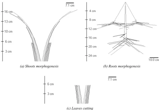
Canopt has been developed since 1996. It models one or more populations of plants that com-pete for resources. The model simulates a mean individual for each population, with compartments for various matters in the plant [9, 10]. The aerial part (the shoots) of the plant is detailed: the growth and senescence of each leaf is considered, as well as its geometry, to get precise photo-synthesis representation for the competition for light (Figure 2a). The roots of the plant are also detailed (Figure 2b), to get more precise representation of the plant uptake in the soil.
Figure 2: Screenshot of a plant simulation with UNIF.
More recently, since 2004, the Canopt and Soilopt models have been coupled to form the GEMINI model. The basic plant representation in Soilopt is now replaced by Canopt, and re-versely, the basic soil representation in Canopt is now replaced by Soilopt [8]. Moreover, modules representing human activity on the plant populations have been introduced, such as cutting, i.e. removing parts of the leaves from the plants at given dates (Figure 2c).
3
Designing a Single Model
The full GEMINI model has presently around 460 equations, which means that some sophisticated structure is necessary to get a maintainable and evolutive model. Object-orientation has been chosen to design the UNIF platform, and is underlying in the development of models with this framework. From now on, the UML 2.0 language [5] will be used to describe the structure of UNIF with class diagrams.
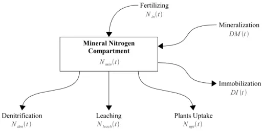
This section presents how to design a single model with UNIF, which means a model that is not decomposed into submodels. The mineral nitrogen compartment of a soil, as it is defined in the Soilopt model, has been chosen as an illustration here, which allows us to introduce first the fundamental functionalities of UNIF. This compartment represents, at time t, an amount Nmin(t) of mineral nitrogen, which can vary by many means (Figure 3):
4
• Fertilizing, which provides a quantity Nin(t) of mineral nitrogen to the soil.
• A mineralization process in the soil, which provides a quantity DM (t) of mineral nitrogen. • An immobilization process in the soil, which takes up a quantity DI(t) of mineral nitrogen. • Denitrification and leaching processes, which take up respectively the quantities Nden(t)
and Nleach(t) from the soil.
• Plants absorption, which takes up a quantity Nupt(t) of mineral nitrogen from the soil.
Figure 3: Fluxes of the mineral nitrogen compartment.
The equation that rules the mineral nitrogen compartment can thus be formulated as follows. δNmin
δt = Nin(t) − Nden(t) − Nleach(t) − Nupt(t) + DM (t) − DI(t) 3.1 Model Structure
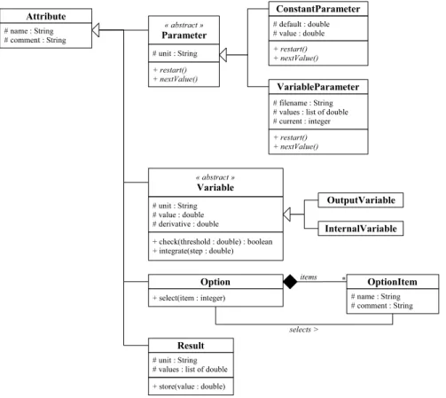
The UNIF framework considers a model as an object with specific attributes (Figure 4):
param-eters that are inputs for the model, they can be either constant or variable (read from a file); integration variables that are the variables ruled by differential equations, they can be either
in-ternal (they are not meant to be visible from outside) or an output of the model; results that trace the evolution of the output variables of the model; and options to select, activate / deactivate... functionalities of the model.
Figure 4: Specific attributes of a model with UNIF.
Research Report FGEP/RR06-10
In our simplistic example, we assume Nin, Nden, Nleach, Nupt, DM and DI to be constant, which means they will be considered as constant parameters of the model in the UNIF framework. The only integration variable of the model is Nmin, which will also be the only output. To create this model in the UNIF framework, it is necessary to create a new class, calledMineralfor in-stance, that inherits from theModelsuperclass provided by UNIF. In this new class, we define the attributesNin,Nden,Nleach,Nupt,DMand DIof classConstantParameter, corresponding to the parameters of the model; the attributeNminof classOutputVariable, corresponding to the integration variable of the model; and the attributeresNminof classResult, corresponding to the output of the model. Here is partially the associated C++ source code.
class Mineral : public Model { protected: ConstantParameter Nin; protected: ConstantParameter Nden; protected: ConstantParameter Nleach; protected: ConstantParameter Nupt; protected: ConstantParameter DM; protected: ConstantParameter DI; protected: OutputVariable Nmin;
protected: Result resNmin;
... };
These attributes will be initialized in the constructor of the class. Mainly, they will be given a name, a comment to explain their function, sometimes a unit... (Figure 5). These informations will be used by the simulator and the user interface. Notice that the initial value of the integration variables is not set in the constructor, but during the initialization step of the simulation, as it will be explained later.
6
3.2 Simulation Sequence
The simulation of a numerical integration model consists in the integration of variables described by differential equations. For the mineral nitrogen compartment, its simulation means computing, for each time step T , the value Nmin(T ).
Nmin(T ) = Z T
T0
δNmin
δt dt+ Nmin(T0)
The integration is discretized using known methods like Euler, Runge-Kutta... The Euler method assumes a constant derivative between two successive time steps T and T+ ∆T .
Nmin(T + ∆T ) = Nmin(T ) + ∆T ×δNmin δt (T )
The4th-order Runge-Kutta method attempts to correct the error made with the Euler method
through a more sophisticated computation, which requires 4 derivatives(ki)i=1..4of the function at different points [7].
Nmin(T + ∆T ) = Nmin(T ) + ∆T × k1+ 2k2+ 2k3+ k4 6
Independently of the integration method, it appears that the evolution of the integration vari-ables is reduced to the computation of their derivatives. Thus, the UNIF simulator will automat-ically simulate a model from the derivatives of its integration variables: each model must have a method namedderivate()where to find the code to compute the derivatives. More precisely, the simulation process is decomposed into five steps for each model (Figure 6).
Figure 6: TheModelclass of UNIF.
• Initialization: The simulator calls theinitialize() me-thod of the model. It initializes the integration variables of the model, thus describing the initial state of the simulated system.
• Pre-integration: Before each integration step, the simulator calls thepreIntegrate()method of the model. The state of the system can be checked to trigger discrete events, e.g. the birth of a new leaf in a plant model.
• Integration / Derivation: At each integration step, the sim-ulator calls thederivate()method of the model. From the derivatives of the variables of the model, the integration method will compute the new state of the variables. Notice that depending on the integration method, thederivate()
method can be called several times in a same integration step.
• Post-integration: After each integration step, the simulator calls the postIntegrate() method of the model. The state of the system can be checked to trigger discrete events. • Termination: The simulator calls the terminate() me-thod of the model. It terminates the simulation of the model. For instance, treatments can be performed on the data col-lected during the simulation.
Research Report FGEP/RR06-10
For the mineral nitrogen compartment, the code of thederivate()method is simply:
void Mineral::derivate(void)
{ Nmin.setDerivative(Nin - Nden - Nleach - Nupt + DM - DI); }
4
Designing a Complex Model
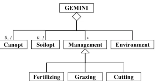
This section presents how to design a complex model with UNIF, which means a model that is decomposed into submodels. We propose to con-sider the whole GEMINI model as an illustration. As mentioned previously, this model is the cou-pling of two models: Canopt and Soilopt. These models are also complex models and they are coupled in GEMINI with other models: an envi-ronmental model and management models
(fer-tilizing, grazing and cutting) (Figure 7). Figure 7:Structure of the GEMINI model. The overall structure of GEMINI only illustrates the composition relationship that can exist between models. Moreover, the relationship is always static in this example. The Canopt model presents other relationships, like inheritance and dynamic composition. Figure 8 details the struc-ture of Canopt.
Figure 8: Structure of the Canopt model.
The model can simulate several populations of plants, and each plant model can have shoots and/or roots submodels. These models are also respectively composed of leaf and root submodels. These models represent elements that will be born during the simulation, and will probably die before the end of the simulation. Leaf and root models will thus be created during the simulation process. Canopt can model various kinds of plants, but only two families of plants have been designed yet: grasses and legumes. The models of these families extend the generic plant model.
4.1 Hierarchical Structure
With the UNIF framework, a model is assumed to be potentially composed of other models, called its children (Figure 9a). This issue is identified as the composite design pattern [4]. There are many ways to implement this pattern. In the UNIF platform, we chose to design a generic class that models a hierarchy (i.e. a tree) of elements (Figure 9b).
8
Figure 9:Models hierarchy with UNIF.
A classical design of generic tree structure would provide a data structure to store the models. But we wanted, in UNIF, a generic tree structure that could be extended such that a model can be a tree of models. That explains the specificity of the generic classTree<T>(Figure 9): a tree does not contain explicitly subtrees (of classTree<T>), but only elements of typeT. However, it is implicitly assumed in the design of the generic class thatTis a tree (i.e. of class Tree<T>). Thus, this generic class, instantiated for theModelclass, is inherited by theModelclass itself.
4.2 Overall Simulation Process
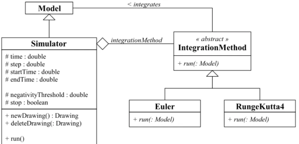
In the UNIF framework, the simulation is controlled by an object of classSimulator. A simu-lator is actually a model: theSimulatorclass inherits from theModelclass (Figure 10). The
Simulatorclass has a specific method, calledrun(), that performs and controls all the steps of the simulation of the model. This method can indifferently use the Euler or Runge-Kutta meth-ods, or any other integration technique. This functionality has been modeled with the well-known
strategy design pattern [4].
Figure 10:TheSimulatorclass of UNIF.
Research Report FGEP/RR06-10
In a complex model, the simulator will be the top-model, e.g. the GEMINI model in our illus-tration. Itsrun()method controls the five steps of the simulation of the top-model (as defined in Section 3.2): initialization, pre-integration, integration / derivation, post-integration, termination. At each one of these phases, the top-model calls the corresponding phase of its submodels. For in-stance, the derivation step of GEMINI consists first in the derivation of its own variables, and then in the derivation (i.e. a call to thederivate()method) of each one of its submodels (Canopt, Soilopt, environment and management models). Recursively, the derivation step of any submodel consists in the derivation of its own submodels. Finally, here is an overview of therun()method of a simulator. stop = false; time = startTime; reserveGraphicalResources(); initializeResults(); restartVariableParameters(); initialize();
while (time < endTime and not stop) { updateVariableParameters();
preIntegrate();
integrationMethod.run(this); // Calls derivate() time += step; checkVariables(negativityThreshold); // Optional postIntegrate(); } terminate(); freeGraphicalResources();
Notice that the five simulation steps mentioned previously are recursive, and that other fully automated and recursive steps may be necessary:
• initializeResults()to prepare the results for data collection; • restartVariableParameters()to initialize the variable parameters;
• updateVariableParameters()to read the next value of each variable parameter; • checkVariables()to check whether a variable becomes negative.
The order by which a model derivates its submodels has not been automated yet. This is a difficult issue, especially when coupling models, that we address in another paper [1]. For instance, the coupling between Canopt and Soilopt requires a precise order to derivate each integration variable of both models. In [1], we propose a new prototype of UNIF with automatic ordering of the derivation process.
5
Graphical User Interface
A model can provide visual simulation with the UNIF framework (Figure 2). For this purpose, a set of abstract classes is available, which makes the code of the simulator and the models fully independent of any graphical user interface (Figure 1).
10
A model can ask for a drawing area (of classDrawing) to the simulator model (Figure 11), by calling itsnewDrawing()method (Figure 10). The simulator delegates then the creation of the drawing to a manager (of classDrawingManager). The simulator is associated with a manager during its construction phase (this is the user interface that creates the simulator, providing thus the manager). Once a model has a drawing area, it is able to perform drawing actions, through theDrawinginterface, that are updated on the screen at the next time step of the simulation. The drawing areas of each model are created in the recursive reserveGraphicalResources()
method (Figure 6). They are deleted in thefreeGraphicalResources()method.
Figure 11:The drawing interface of UNIF.
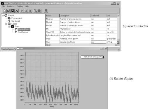
Only a Windows interface has been developed yet, with the Borland C++ Builder environment. This interface allows to activate / deactivate submodels (left of Figure 12a), to modify the value or the input file of each parameter (right of Figure 12a), to select options (Figure 12b), and after the simulation, to select results (Figure 13a) for display (Figure 13b) or for export.
Figure 12:Screenshot of a model configuration with UNIF.
Research Report FGEP/RR06-10
Figure 13:Screenshot of results display with UNIF.
Conclusion
The UNIF framework allows the design and the simulation of numerical integration models, i.e. models mainly formulated with ordinary differential equations. The simulator is fully independent of the integration method, which allows to select the adequate technique for a specific model. Moreover, the integrity of the variables of a model (mainly their divergence) can be checked at any step of the simulation. Discrete events can also be introduced in the simulation process: events can be triggered before and after each integration step.
It is possible to design complex models, structured in a hierarchy of submodels. This struc-ture is usually static, i.e. it remains the same during the whole simulation, but submodels can be dynamically added to a model during the simulation (e.g. a plant that produces a new leaf). The integration process is partially automatic, and is actually able to manage the simulation of a hierarchy of models. However, further investigations must be conducted on:
• How to provide some flexibility in the granularity of the models ? How to replace a submodel by another one, with the same function, but with a different level of details ? This implies to think of means to achieve the coupling of models, and more precisely, on means to represent the interface between two models.
• How to allow the coupling of models ? If we assume that two models have been developed independently with the UNIF framework, how to make their coupling possible ? The main difficulty that appears is the reordering of the integration variables of both models for the derivation process.
We propose a new prototype of the UNIF framework that attempts to address these two main issues [1]. We use the coupling of Canopt and Soilopt as an illustration for these problems, and present an experiment based on simplified versions of these models to test our prototype.
12
References
[1] Bruno Bachelet, Jean-Christophe Gay, and Vincent Maire. Coupling Numerical Integra-tion Models: Granularity and ComputaIntegra-tional Sequence. Technical report, INRA / FGEP, Clermont-Ferrand, France, 2006.
[2] François E. Cellier and Ernesto Kofman. Continuous System Simulation. Springer, 2005. [3] Sébastien Fontaine and Sébastien Barot. Size and Functional Diversity of Microbe
Popu-lations Control Plant Persistence and Long-Term Soil Carbon Accumulation. In Ecology
Letters, volume 8, pages 1075–1087. Blackwell Publishing Ltd, 2005.
[4] Erich Gamma, Richard Helm, Ralph Johnson, and John Vlissides. Design Patterns: Elements
of Reusable Object-Oriented Software. Addison-Wesley, 1995.
[5] Object Management Group. Unified Modeling Language: Superstructure (Version 2).
http://www.omg.org/cgi-bin/doc?ptc/2003-08-02, 2003.
[6] Pierre Loiseau and Yannick Bergia. Modélisation et simulation des flux d’azote et de carbone dans les sols prairiaux. Technical report, INRA / FGEP, Clermont-Ferrand, France, 1998. [7] William H. Press, Saul A. Teukolsky, William T. Vetterling, and Brian P. Flannery. Numerical
Recipes in C - The Art of Scientific Computing, 2nd Edition. Cambridge University Press,
1992.
[8] Jean-François Soussana and Jean-Philippe Brassier. Implémentation des équations d’in-terface entre un modèle de sol prairial et un modèle de peuplement végétal. Technical report, INRA / FGEP, Clermont-Ferrand, France, 2000.
[9] J.F. Soussana, F. Teyssonneyre, and J. Thiéry. Un modèle dynamique d’allocation basé sur l’hypothèse d’une co-limitation de la croissance végétale par les absorptions de lumière et d’azote. In Fonctionnement des peuplements végétaux sous contraintes environnementales, pages 87–116. INRA, France, 2000.
[10] J.F. Soussana, F. Teyssonneyre, and J. Thiéry. Un modèle simulant les compétitions pour la lumière et pour l’azote entre espèces herbacées à croissance clonale. In Fonctionnement des
peuplements végétaux sous contraintes environnementales, pages 325–350. INRA, France,
2000.
Research Report FGEP/RR06-10