Box modeling of the Eastern Mediterranean sea
The MIT Faculty has made this article openly available. Please share
how this access benefits you. Your story matters.
Citation Ashkenazy, Yosef, Peter H. Stone, and Paola Malanotte-Rizzoli. "Box modeling of the Eastern Mediterranean sea." Physica A: Statistical Mechanics and its Applications 391:4 (February 2012), pp.1519-1531.
As Published http://dx.doi.org/10.1016/j.physa.2011.08.026
Publisher Elsevier
Version Author's final manuscript
Citable link http://hdl.handle.net/1721.1/103955
Terms of Use Creative Commons Attribution-NonCommercial-NoDerivs License
Box Modeling of the Eastern Mediterranean Sea
Yosef Ashkenazya,∗, Peter Stoneb, Paola Malanotte-Rizzolib
a
Solar Energy and Environmental Physics, BIDR, Ben-Gurion University, Israel b
Department of Earth Atmospheric and Planetary Sciences, Massachusetts Institute of Technology, Cambridge, MA 02139
Abstract
In ∼1990 a new source of deep water formation in the Eastern Mediterranean was found in the southern part of the Aegean sea. Till then, the only source of deep water formation in the Eastern Mediterranean was in the Adriatic sea; the rate of the deep water formation of the new Aegean source is 1 Sv, three times larger than the Adriatic source. We develop a simple three box-model to study the stability of the thermohaline circulation of the Eastern Mediter-ranean sea. The three boxes represent the Adriatic sea, Aegean sea, and the Ionian seas. The boxes exchange heat and salinity and may be described by a set of nonlinear differential equations. We analyze these equations and find that the system may have one, two, or four stable flux states. We conjecture that the change in the deep water formation in the Eastern Mediterranean sea is attributed to a switch between the different states on the thermoha-line circulation; this switch may result from decreased temperature and/or increased salinity over the Aegean sea.
Keywords: Deep water formation, Box model, Mediterranean sea, Eastern Mediterranean Transition
1. Introduction
Observations of a major increase in the amount of bottom water forma-tion and discharge from the Aegean sea [1, 2, 3, 4] raise the possibility that
∗Corresponding author address: Department of Solar Energy and Environmen-tal Physics, BIDR, Ben-Gurion University, Midreshet Ben-Gurion 84990, Israel. Tel.:+972 8 6596858; fax:+972 8 6596921 .
the circulations in the Eastern Mediterranean are unstable and subject to sudden changes. A major change in the deep water formation in the Eastern Mediterranean sea occurred ∼1990, basically, in the vicinity of the Adriatic-Aegean-Ionian seas [2, 5, 6, 3, 1, 4]. Hydrographic surveys since early last century [7] indicated that the dominant source region for deep water over the entire Eastern Mediterranean, was the Adriatic sea; see Fig. 1. Waters outflowing from the Adriatic were deposited in the bottom of the Ionian sea [8]; then they spread southward and eastward [9, 10]. The deep water over-turning time was approximately 100 years with an average formation rate of
0.3 Sv = 0.3 ×10⁶ m3s−1 [11]. An additional, much more dominant, source
of deep water was found in a hydrographic survey during 1995 [1]. The new source was found in the southern part of the Aegean sea and has an average outflow rate of about 1 Sv. A recent study suggested that the change in the thermohaline circulations of the Eastern Mediterranean sea actually started before October 1991 [3]. The characteristics of the thermohaline circulation of the Eastern Mediterranean sea continued to change after 1995—Manca et
al. [12] and Theocharis et al. [13] reported the weakening of the Aegean
source of deep water and the strengthening of the Adriatic source during 1997-1999. These changes may be attributed to changes in the surface fluxes and inflows to the Adriatic, Ionian and Aegean basins.
Several explanations have been suggested for the change in the deep wa-ter formation of the Easwa-tern Mediwa-terranean sea. One study suggested that enhanced net evaporation led to the formation of the new Aegean source [14]. In addition, the north Eastern Mediterranean experienced some cold winters during the 1987-1995 period and these have been associated with changes in the thermohaline circulation throughout the region [15, 16, 17]. However, the lack of oceanic data during 1987-1995 makes it difficult to uncover the exact cause for the formation of the new Aegean source. Ocean General Circula-tion Models (OGCMs) have been used to better understand the possibilities which led to the formation of the new Aegean source. For example, changes in the wind stress over the Aegean basin were related, using an OGCM, to the formation of the new Aegean source [18]. Dry and cold winters of 1987, 1992-93, were also related, using an OGCM, to the formation of the new Aegean source [5]. These studies based their numerical simulations on re-analysis data and didn’t fully reproduce the entire Aegean source pattern. Wu et al. [19], on the other hand, forced an OGCM by eight consecutive cold winters (from 1987 to 1995) over the Aegean basin. They showed that a
formation over the Aegean; winter sea surface temperature over the Aegean
sea was observed to be up to 3 ◦C colder than the climatological average
[20, 17]; the box model described below is also based on this work, where we assign the Aegean box with colder temperatures to explain the Eastern Mediter-ranean Transient (EMT). Stratford and Haines [21] also performed OGCM simulations and suggested that a combination of a few cold winters together with changes in the wind stress over the Eastern Mediterranean underlies the formation of the Aegean source.
The idea that density-driven circulations in the ocean could, under a given set of boundary conditions, display more than one equilibrium state, and therefore may have a behavior like that recently observed in the Aegean sea, was first put forth by Stommel [22]. He illustrated the behavior with a very simple two-box model of the thermohaline circulation. The two equilibrium states that he found in his simple box model have since been found in simu-lations of the North Atlantic thermohaline circulation with the most sophis-ticated coupled atmosphere-ocean general circulation models [e.g., 23, 24]. These results lend considerable credibility to Stommel’s box model. How-ever, there is nothing in his model that limits its applicability to large-scale circulations in the North Atlantic — indeed in his paper he even suggested that it might be relevant to the Mediterranean sea. Here we apply the same basic ideas as Stommel’s to develop a box model of the Eastern Mediter-ranean, and explore what the possible multiple equilibrium states are, and what their stability characteristics might be.
Previous studies have pointed out the importance of the box models in the understanding of the water circulation in the Mediterranean sea. E.g., Tziperman and Speer [25] used a simple box model to study the seasonal effect on the formation of deep water over the Mediterranean sea. Another study [chapter 3 in 26] used a 2 × 2 box model as well as 6 × 4 box model to study the deep water formation over an Eastern basin of the Mediterranean sea (in the Adriatic sea) and over a Western basin of the Mediterranean sea (in the Gulf of Lion); the influence of the incoming Atlantic water and the outgoing Levantine Intermediate Water was also considered. They found, in the framework of their box models, multiple equilibria stable flux states in the Western Mediterranean (Golf of Lion) and/or in the Eastern Mediterranean sea (Adriatic sea); see also [27]. However, these studies didn’t include the Aegean sea in their models, and thus they are inappropriate to study the EMT.
the possible causes for the recent changes in the thermohaline circulation of the Eastern Mediterranean sea. The simplicity of the model allows us to analytically analyze the steady states of the thermohaline circulation and the stability of these states. We show that the Aegean bottom water forma-tion can be driven by cold atmospheric temperature and changes in the net evaporation over the Aegean.
2. Three box model of the Eastern Mediterranean Sea
We represent the Adriatic sea, the Ionian sea, and the Aegean sea, by three boxes, a, b, c respectively. All three boxes are forced by surface fluxes of heat and salinity and the boxes are assumed to be well mixed, so that their states can be described by a single temperature and salinity for each box.
The flux between Box a and Box b is q1 (representing Ionian-Adriatic flux)
and the flux between Box c and Box b is q2 (representing the Ionian-Aegean
flux); see Fig. 1. The boxes “interact” through “pipes” with the fluxes q1
and q2. The volumes of the boxes, Va,b,c, are kept fixed. Positive q1,2 indicates
sinking in box qa,c and deep flow from the Adriatic/Aegean to the Ionian while
negative qa,c indicates sinking in the Ionian and deep flow from the Ionian to the
Adriatic/Aegean.
The circulations between the boxes are assumed to be proportional to the density gradients between the boxes [22], and with this parameterization the state of the system can be described by conservation equations for heat and salinity for each box, giving a total of six equations for the temperatures and salinities of the three boxes. The equations are nonlinear because of the nonlinear advection of heat and salinity between the boxes, and this nonlinearity give rise to the possibility of multiple equilibrium states.
The fluxes q1 and q2 are proportional to the density gradients between
the boxes,
q1 = k1[α(Tb− Ta) − β(Sb− Sa)], (1)
q2 = k2[α(Tb− Tc) − β(Sb− Sc)], (2)
where Ta,b,c are the temperatures of the boxes, Sa,b,c are the salinities of the
boxes, α and β are the thermal and haline expansion coefficients, and k1,2 are
flux constants. We assume that the total salt of the three boxes is conserved. The net virtual salinity fluxes out of boxes a and c are HS1 and HS2, and the
equivalent to positive net precipitation minus evaporation (or positive freshwater flux), in our case making boxes a or c fresher compare to box b. We define the following variables and constants: T1 ≡ Tb− Ta, T2 ≡ Tb− Tc, S1 ≡ Sb− Sa,
S2 ≡ Sb− Sc, hS1 ≡ HS1Va, hS2 ≡ HS2Vc, and hTa,b,c ≡ HTa,b,c/Cpρ0Va,b,c (Cp
is the heat capacity per unit mass of water and ρ0 is the average sea water
density). Following [22, 28, 29] the salt and heat equations can be written as, ∂Sa ∂t = − hS1 Va − |q1| Va (Sa− Sb), (3) ∂Sc ∂t = − hS2 Vc − |q2| Vc (Sc− Sb), (4) ∂Sb ∂t = hS1 Vb + hS2 Vb − |q1| Vb (Sb− Sa) − |q2| Vb (Sb − Sc), (5) ∂Ta ∂t = hTa − |q1| Va (Ta− Tb), (6) ∂Tc ∂t = hTc − |q2| Vc (Tc − Tb), (7) ∂Tb ∂t = hTb − |q1| Vb (Tb− Ta) − |q2| Vb (Tb − Tc). (8)
These equations describe the amount of salt and heat entering/leaving the boxes through the pipes plus the contribution of the surface fluxes. It is easy to show that the total salt content of the boxes is preserved, i.e., ∂t(VaSa+
VbSb + VcSc) = 0.
After a few algebraic operations the system reduces to four equations for the temperature and salinity gradients
∂T1 ∂t = hTb− hTa − µ 1 Va + 1 Vb ¶ |q1|T1− |q2| Vb T2, (9) ∂T2 ∂t = hTb− hTc − |q1| Vb T1 − µ 1 Vc + 1 Vb ¶ |q2|T2, (10) ∂q1 ∂t = k1 · α(hTb − hTa) − βhS1 µ 1 Va + 1 Vb ¶ − βhS2 Vb ¸ −µ 1 Va + 1 Vb ¶ |q1|q1− k1 k2 1 Vb |q2|q2, (11) ∂q2 ∂t = k2 · α(hTb − hTc) − β hS1 Vb − βhS2 µ 1 Vc + 1 Vb ¶¸
−k2 k1 1 Vb |q1|q1− µ 1 Vc + 1 Vb ¶ |q2|q2. (12)
These equations are decoupled from two additional equations for the mean temperature and salinity. To obtain the fixed points of the system we set the left hand side to zero, i.e., ∂T1,2/∂t = 0 and ∂q1,2/∂t = 0. From the
temperature equations we then obtain hTb− hTa = µ 1 Va + 1 Vb ¶ |q1|T1 + |q2| Vb T2, (13) hTb− hTc = |q1| Vb T1+ µ 1 Vc + 1 Vb ¶ |q2|T2. (14)
Substituting for the surface heat fluxes in Eqs. (11) and (12) lead to
ki(α|qi|Ti− βhSi) = |qi|qi (15)
where i = 1, 2.
For qi > 0 there are two solutions,
qi1,2 = 1 2kiαTi à 1 ± s 1 − 4kiβhSi (kiαTi)2 ! , (16) if (kiαTi)2 > 4kiβhSi. (17)
For qi < 0, there is one negative solution,
q3 i = 1 2kiαTi à 1 − s 1 + 4kiβhSi (kiαTi)2 ! . (18)
If the salinity flux is negative (hSi < 0) just the q
1
i solution is valid. In
the above solutions we assume, consistent with the climatology, that the temperature gradients are positive; i.e., T1,2 > 0. The q31,2 solution is the
salinity dominant stable flux state while q1
1,2 is the temperature dominant
stable flux state. q1
1,2 corresponds to sinking in boxes a and c while q1,23
corresponds to sinking in box b. As in Stommel’s model q2
1,2 is an unstable
state.
In the following, the terms “thermally” and “salinity” dominant states are frequently used and we thus elaborate on this terminology. A “thermally dom-inant” state is usually reffed to a situation is which one of the boxes is fresher
than its counterpart where it is colder enough than its counterpart such that sinking occurs in it, sometimes despite the fresher water of the box; hence the term “thermally dominant”, to indicate that the sinking occurs due to thermal (temperature) effects. In other cases, one box may be warmer than its counter-part, making the box’s water lighter; still since its salinity is large enough than its counterpart, sinking will occur in the warmer box—the term “salinity dominant” reflects the fact the sinking occurred due to the high salinity.
In some cases the salinity flux hSi is relatively small, i.e.,
4kiβ|hSi| ≪ (kiαTi)
2
. (19)
Under this condition it is possible to simplify the flux steady states, q1 i ≈ kiαTi, (20) q2 i ≈ βhSi αTi , (21) q3 i ≈ − βhSi αTi . (22)
To explicitly know the flux solutions it is necessary to evaluate the temper-ature gradients T1 and T2. In the following subsections we will consider two
different scenarios: (i) The temperatures of the boxes are strongly coupled to the atmospheric apparent temperatures, i.e., the relaxation is assumed to be immediate and the temperatures of the boxes are thus assumed to be fixed and equal to the atmospheric temperatures. (ii) The temperatures of the boxes are assumed to be variable.
2.1. Fixed temperatures
As a first approximation we assume that the atmosphere is strongly cou-pled to the ocean. Thus, we assume that the temperatures of the different boxes are fixed and equal to the atmospheric (climatological) temperatures; the following analysis would however be valid for any fixed box temperatures and not just for atmospheric climatological temperatures. The three box system in this special case has already been analyzed by Welander [30]. In this case, the flux steady state solutions are given in Eqs. (15) where T1,2 are
constants. These are two independent solutions for q1 and q2 and each has
either one or three solutions [Eqs. (16)-(18)]. It follows that the equilibrium states of the Adriatic and Aegean seas (boxes a and c) interact independently with the Ionian sea (box b), and in fact in equilibrium the model decouples
into two separate two-box models, each identical to the original Stommel two-box model [30]. Thus, for example, there are two possible stable states for the Adriatic, one with strong bottom water formation, and one without.
All together there are either one, three, or nine fixed points; i.e., (q3 1, q 3 2), (q3 1, q 1,2,3 2 ) or (q 1,2,3 1 , q 3 2), and (q 1,2,3 1 , q 1,2,3
2 ) respectively. For the nine fixed
points case, it is possible to show that (i) four of these fixed points are stable, i.e., (q1,31 , q
1,3
2 ), (ii) four are semi-stable (saddle points), i.e., (q 2 1, q 1,3 2 ) and (q11,3, q 2
2), and (iii) one is unstable, i.e., (q 2 1, q
2
2). In addition, there are
no spiral modes in the system — there is only simple damping or simple repelling of these fixed points.
Although the fixed points of Eqs. (15) are independent of each other their stabilities depend on each other. To study the basin of attractions of the stable fixed points we first set dq1/dt (or dq2/dt) to zero and then find
the dependence of q1 on q2 (or vice versa); a similar stability analysis, using
different variables, was performed by Welander [30]. The “stability lines” are the lines for which q1 (or q2) is minimal or maximal. In Fig. 2 we present two
examples of the fixed points with their basins of attraction. Figure 2a shows the situation when the salinity flux forcing is weak and positive (hSi > 0) for
which there are nine fixed points. Figure. 2b shows the situation when the salinity flux forcing of the Aegean box (box c) is weak but negative (hS1 > 0,
hS2 < 0) for which there are three fixed points. We assume that the volume
of the Ionian is ten times larger than the volume of the Aegean, and that the Aegean is twice the volume of the Adriatic. These ratios are approximately realistic (Table 1), and illustrate some of the possible ways in which the basins can interact. In Fig. 2a (positive salinity flux) the four heavy dots indicate the stable equilibria of the system. One has strong bottom water formation in both the Adriatic and the Aegean; one has no bottom water formation in either (actually there is a slightly negative amount of bottom water formation in this state); and the other two have strong bottom water formations in one of the seas, but not the other. The shading indicates the attractor basin for each equilibrium. In the case with negative salinity flux forcing for the Aegean (Fig. 2b), two of the stable equilibria have disappeared, and two remain. In one there is strong bottom water formation only in the Aegean, and in the other there is strong bottom water formation in both basins. In effect, the negative salinity forcing of the Aegean has, in this case, eliminated the states with weak bottom water formation in the Aegean. Thus, changes in the salinity flux forcing of the basins may cause drastic changes in the stability of the different basins.
In many cases it is useful to construct a pseudo-potential to describe the system. For the present case, it is possible to show that such a potential cannot be constructed. However, for the case for which Vb ≫ Va,c (as for the
present system), Eqs. (1),(2) can be written in form of a pseudo-potential φ(q1, q2), φ(q1, q2) = 1 Va [|q1|( q2 1 3 − q1 2k1αT1) + k1βhS1q1] + 1 Vc [|q2|( q2 2 3 − q2 2k2αT2) + k2βhS2q2], (23)
for which the time derivative of q = (q1, q2) is
∂q
∂t = −∇φ(q1, q2). (24)
The potentials for the cases shown in Fig. 2 are shown in Fig. 3. The potentials shown in Fig. 3 are more informative since they show the relative stability of the different fixed points while this information is not included in Fig. 2.
2.2. Variable temperatures
Here we assume that the ocean temperatures are not so strongly coupled to the atmospheric temperatures and that the relaxation time for the tem-perature of the different boxes is finite. Following Haney [31] we parametrize the heat flux of the boxes as,
hTj =
λ Dj
(T∗
j − Tj) (25)
where j = a, b, c; λ is the relaxation constant (λ = 8 × 10⁻⁶m/s) [31], D j is
the depth of the different boxes, and T∗
j is the apparent atmospheric
temper-ature of the different boxes. It follows from the equilibrium conditions [Eqs. (13),(14)] that T1 = T1∗− 1 λ µ Da Va +Db Vb ¶ |q1|T1− 1 λ Db Vb |q2|T2, (26) T2 = T2∗− 1 λ Db Vb |q1|T1− 1 λ µ Dc Vc +Db Vb ¶ |q2|T2. (27)
After inserting into Eqs. (26),(27) the expressions for the fluxes q1(T1) and
q2(T2) [Eqs. (16),(18)], we are left with two high order coupled equations
for the equilibrium temperatures T1 and T2. In the following we will use
the approximations [Eqs. (20),(22)] to solve the temperature equations [Eqs. (26),(27)]. We will consider three cases: (i) both fluxes are salinity dominant, i.e., q1 < 0 and q2 < 0; (ii) one of the fluxes is salinity dominant and the
other is thermally dominant, e.g., q1 < 0, and q2 > 0 ; (iii) both fluxes are
thermally dominant, i.e., q1 > 0, and q2 > 0.
2.2.1. Salinity dominant fluxes
For the salinity dominant fluxes q1,2 < 0, and the |qi|Ti (i = 1, 2) term in
Eqs. (26),(27) may be approximated as βhSi/α [Eq. (22)]; i.e.,
T1 = T1∗− 1 λ β α ·µ Da Va +Db Vb ¶ hS1 + Db Vb hS2 ¸ , (28) T2 = T2∗− 1 λ β α · Db Vb hS1 + µ Dc Vc +Db Vb ¶ hS2 ¸ . (29)
The second term on the right hand side is the correction to the apparent
temperatures T∗
1,2. Since the second term on the right hand side is generally
much smaller than the first term on the right hand side, the most basic approximation is Ti ≈ Ti∗, i.e., the temperatures of the boxes are equal to
the apparent temperatures, as in the previous sub-section. 2.2.2. Salinity dominant flux and thermally dominant flux
We consider the case where one of the fluxes is salinity dominant and the other is thermally dominant, e.g., q1 < 0 and q2 > 0. We approximate
|q1|T1 ≈ βhS1/α and |q2|T2 ≈ k2αT
2
2 [Eqs. (20),(22)]. From Eqs. (26),(27)
we obtain T2 2 + 1 k2 A2T2− 1 k2 A2T2∗+ 1 k2 β α2B2hS1 = 0, (30) where A1 = λ α(Da Va + Db Vb) , (31) A2 = λ α(Dc Vc + Db Vb) , (32) B1 = Db/Vb Da Va + Db Vb , (33)
B2 = Db/Vb Dc Vc + Db Vb . (34)
This is a quadratic equation with the solution T2 = 1 2k2 [−A2+ q A2 2+ 4k2(A2T2∗− B2βhS1/α 2)]. (35)
Note that the larger solution for Eq. (30) is chosen to be consistent with the thermally dominant flux q2 > 0. Once T2 is known it is possible to find all
the other variables, q2 [Eq. (20)], T1 [Eqs. (22),(26)], and q1 [Eq. (22)]. In
the case where q1 > 0 and q2 < 0, it is possible to obtain the solution by
replacing the subscript 2 by 1 and vice versa. 2.2.3. Thermally dominant fluxes
The most complex case is when both the Adriatic and the Aegean have thermally dominant fluxes; i.e., q1 > 0 and q2 > 0. In that case we use the
approximations |q1|T1 ≈ k1αT12 and |q2|T2 ≈ k2αT22 [Eq. (20)]. Then Eqs.
(26),(27) can be written as,
k1T12+ A1(T1− T1∗) + k2B1T22 = 0, (36)
k2T22+ A2(T2− T2∗) + k1B2T12 = 0, (37)
where A1,2 and B1,2are defined above [Eqs. (31)-(34)]. This leads to a fourth
order equation for T1,
[k1T12(B2− 1 B1 ) − A1 B1 (T1− T1∗) − A2T2∗] 2 − A 2 2 k2B1 [−k1T12+ A1(T1∗− T1)] = 0. (38)
This equation can be solved by neglecting the term k1T12(B2 − B1
1) on the
left hand side—this term is small for the box model setting of the Eastern Mediterranean described below. Then we are left with a quadratic equation
C1T 2
1 + C2T1+ C3 = 0 (39)
with the solution,
T1 = 1 2C1 (−C2+ q C2 2 − 4C1C3), (40)
where C1 = k2A21+ k1A22B1, (41) C2 = −2k2A21T1∗+ 2k2A1A2B1T2∗+ A1A22B1, (42) C3 = k2A21T1∗ 2 − 2k2A1A2B1T1∗T2∗ +k2A22B 2 1T2∗ 2 − A1A22B1T1∗. (43)
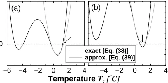
In Eq. (40) we choose the the larger solution, i.e., with positive square-root, since it is closer to the apparent atmospheric temperature — our assumption is that the box temperature relaxes to be as close as possible to the apparent forcing temperature. Eq. (40) is thus an approximation for the largest
solu-tion for the more complex Eq. (38); see Fig. 4a. When C2
2 < 4C1C3 there is
no real solution to Eq. (39). However, the temperature gradient T1does exist
in the more complex Eq. (38). We choose the temperature gradient at the
minimum of the parabola of Eq. (39), T1 = −C2/2C1, as the approximated
solution for Eq. (38); see Fig. 4b. T2 can be found in a similar way; i.e., by
changing the subscript 1 in Eqs. (41)-(43) to 2 and vice versa. Then, the fluxes q1,2 can be obtain using the approximations, qi ≈ kiαTi (i = 1, 2).
3. Application to the Eastern Mediterranean
3.1. Scenarios regarding the Eastern Mediterranean Transient
Below we suggest possible scenarios regarding the EMT based on the three box model analyzed above. A basic scenario may be associated with rapid and strong perturbation that excites the system from one stable thermohaline state to another. Such a scenario may be easily explained using the potential depicted in Fig. 3a. Point A in Fig. 3a may be associated with deep water formation prior to 1990 (before the EMT), where the only source of deep
water was in the Adriatic sea (i.e., q1 ≈ 0.3 Sv and q2 ≈ 0). Making the
Aegean basin temporarily saltier (i.e., by decreasing the virtual surface salinity flux hS2 as a result of reduced exported salt out of the Aegean) can switch the
thermohaline state from Point A to Point B (Fig. 3a). At this (transient) point there are two dominant sources of deep water formation, a relatively weak Adriatic source and a much stronger one at the Aegean sea. Once at Point B, an additional transient (perturbation) warming over the Adriatic can further easily switch the thermohaline state to Point C in Fig. 3a at which there is only one dominant source of deep water at the Aegean sea. The transition from Point A to Point B and from Point B to Point C is
relatively easy as small perturbation is needed for the switch. However the transition from either Point B or C to Point A is more difficult to obtain as a large perturbation is needed. This will lead to asymmetry in the transition— quick transition and formation of the new Aegean source of deep water and a much slower transition back to the only (old) source of deep water in the Adriatic sea. The scenario described above is however less probable as one would expect to observe the Aegean source of deep water even before the EMT. Yet, it is possible to construct another potential in which Points A and D in Fig. 3a are deeper than Points B and C, such that the Aegean source of deep water will be less probable to achieve. In addition, the transition from Point A to Point C may go through Point D instead of Point B, meaning that before the Aegean sea becomes the only source of deep water both basins did not have a source of deep water.
A second scenario regards to changes in the heat and salinity fluxes over the Adriatic, Ionian, and Aegean seas. In this scenario a more permanent change is assumed to occur such that the system can switch from a four stable fixed points situation (Fig. 3a) to a situation with only two stable fixed points (Fig. 3b). First, as in the first scenario described above, the EMT state is at Point A in Fig. 3a. Then a prolonged decrease in the virtual salinity flux over the Aegean (i.e., decrease in hS2 that makes the Aegean saltier) can lead
to denser Aegean water such that the salinity dominant state with sinking in the Ionian is diminished, leaving the Aegean-Ionian basins with the thermally dominant state, with sinking in the Aegean and significant flux between the Aegean and Ionian seas. This situation is depicted in Fig. 3b. Here, the Adriatic source of bottom water can be either as before or can switch to the salinity dominant state with almost zero flux between the Adriatic and Ionian seas. The transition between the salinity dominant and thermally dominant states of the Adriatic sea does not require a large change in the surface fluxes.
The scenario described above can be linked to the previous explanations of the EMT. Specifically, the deep water formation in the Aegean sea was associated with changes in wind patterns [4, 18, 21]. It was suggested [4] that these changes in wind patterns induced a change in the upper thermocline circulation which produced a three-lobe anticyclonic region in the Levantine basin. This anticyclonic region blocks the traditional westbound pathway of Levantine Intermediate Water (LIW) which is veered around the anti-cyclones in a local recirculation pattern. A branch of LIW is veered into the Aegean sea through one of the straits, thus increasing the salinity above the
normal values of Cretan Surface Water. This increased the interior salinity such that under the abnormal cooling of the 90s in the Aegean sea consequent formation of deep water occurred. Since the box model presented above does not incorporate winds, the increase in Aegean salinity due to wind changes may be be incorporated through the surface salinity flux over the Aegean, which together with heat loss may have led to switch the system as described above and depicted in Fig. 3.
The scenarios described in this subsection have been demonstrated, for simplicity, under the assumption of fixed box temperatures (Section 2.1). Still, we conjecture that these scenarios will be valid even when this assumption is relaxed, as our numerical results shown below and the semi-numerical model’s solutions also exhibited multiple states and hysteresis behavior. In addition, other scenarios for switching between the states are possible.
3.2. Parameter choices
The parameter values used in our model are given in the Table 1. The Io-nian sea basin is taken to be between 15.5E-23E and 30N-40.5N, the Aegean basin between 23E-27E and 35N-41.5N, and Adriatic basin between 12E-20E 42N-46N and 15E-12E-20E 40.5N-42N; see Fig. 1. The dimensions (volume and depth) of the different boxes were measured using the Mediterranean
bathymetry map (the Mediterranean Ocean Data-Base, MODB, http://modb.oce.ulg.ac.be/modb/ Note that the depths are the mean depths. The evaporation and precipitation
over the boxes are based on the Dasilva 94 Atlas (http://ingrid.ldeo.columbia.edu/SOURCES/). The river run-off to the boxes are based on the Global Runoff Data Center
database (http://www.bafg.de/). The virtual salinity fluxes, HS1 and HS2,
are related to the annual average precipitation plus river runoff minus evap-oration, P + R − E, over the different basins, by the general relation
HS = S0(P + R − E)/D − c, (44)
where S0 is the standard sea water salinity, D is the depth of the box, and
c includes all non-surface flows, such as the inflow of fresher Atlantic water and saltier Levantine water. Unfortunately the net flows into the different basins are not well known. One problem, as shown by [12] and [32] recently, is that the net inflow of salinity to the Ionian from the Levantine basin has substantial interannual variations. Another problem is that P + R − E for the Aegean as estimated from the sources cited above is small compared to the errors, such that even its sign is uncertain. Based on this observation we
refrain from using a specific value of surface salinity flux but rather examine
a range of parameters. When varying HS1 and HS2 in the solutions, we
are perturbing the net flows of virtual salinity between just the three basins themselves, and are assuming no perturbations to the total flow of virtual salinity into the three basins.
The most critical parameters are k1 and k2. We approximate k1 and k2
using the average temperature and salinity over the surface layer of 200 m depth; we use the climatological data of MODB to compute these averages: the mean salinity of the upper 200 m of the Adriatic, Ionian, and Aegean basins is 38.59, 38.65, and 38.99 psu respectively, where the mean tempera-ture of the upper 200 m of these basins is listed in Table 1. Since the average temperatures and salinities are based on climatological data they describe
the situation prior to 1990. The Adriatic-Ionian constant, k1, may be
ap-proximated by Eq. (1) using the observed flux of 0.3 Sv. However, since the (small) Aegean-Ionian flux pre 1990 is unknown we are unable to
approxi-mate k2. On the other hand, it was reported that the temperature over the
Aegean basin dropped by 2 ◦C during several winters after 1990 [16, 19]. We
note that most bottom water is formed in winter. These facts enable us to estimate the Aegean-Ionian constant, k2. We first decrease the climatological
average temperature by 2 ◦C and then use the reported 1 Sv in Eq. (2) to
compute k2. Thus k2 is based on the post 1990 conditions. Under the current
setting, the Aegean constant k2 is about 1.6 times larger than the Adriatic
constant k11.
The apparent temperatures T∗
a,b,c used in Eq. (25) are approximated as
the average temperatures over the surface layer of 200 m depth (using the MODB), in accordance with the strong coupling approximation. This choice in effect means that we are finding the first order solution in a perturbation expansion in which we assume that the difference between the apparent at-mospheric temperature and the sea surface temperature is small. The fixed temperature approximation corresponds to the zero order solution.
1Note that k
1, and k2 values are calculated based on the upper ocean temperature and salinity. Ideally one would like to consider the total volume temperature and salinity averages. However, this approach is not applicable for the Eastern Mediterranean since the Ionian box is much deeper than the Adriatic and the Aegean boxes and thus contains the more dense water. Using this greater density of the Ionian would lead to negative k1,2 in Eqs. (1), (2), i.e., deep water formation in the Ionian, in contrast with observations.
3.3. Sensitivity tests
To examine the validity of the proposed box model to the Eastern Mediter-ranean we have performed sensitivity tests in which the fluxes q1,2 are
cal-culated as a function of the apparent temperatures and the surface salinity fluxes; the numerically calculated fluxes are shown where the analytical ap-proximations under the assumption of variable temperatures exhibited simi-lar results to the numerical ones.
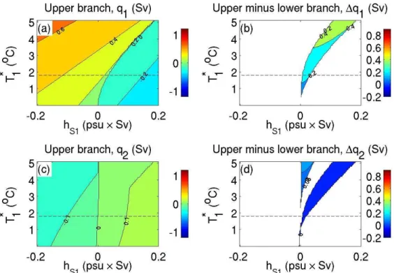
In Fig. 5 we depict the fluxes q1,2 as a function of hS1 and T1∗ where
we assume that hS2 = 0 and the apparent temperature T
∗
2 is based on the
values given in Table 1. Since the model may lead to two different values of
q1 we present the upper branch and the difference between the upper branch
and lower branch in two different panels, Fig. 5a,b—when the upper and the lower branches are identical the difference is obviously zero, indicating
the lack of multiple states. The fluxes q1 (panel a) and q2 (panel c) fall
within the range of observed values for the observed apparent temperature (indicated by the dashed line). For approximately zero surface salinity flux, hS1 ≈ 0 the Adriatic-Ionian flux is q1 ≈ 0.3 Sv, and the Aegean-Ionian flux
is small (q1 ≈ 0.17 Sv), both values roughly consistent with the Eastern
Mediterranean circulation prior to the EMT. The salinity dominant state, with sinking in the Ionian (box B), is found in the lower right corner of Fig. 5a, i.e., for positive Adriatic-Ionian surface salinity flux and relatively small temperature difference between the Adriatic and Ionian boxes. The positive surface salinity flux (net precipitation over the Adriatic and compensating net evaporation over the Ionian) makes the Adriatic box fresher and the Ionian box saltier, leading to sinking in the Ionian box.
It is possible to observe two states of thermohaline circulation for positive hS1, where the region of bi-stability is larger for greater apparent temperature
T∗
1 (Fig. 5b). The bi-stability region is different when assuming different hS2
and T∗ 2.
It is important to note the small variation in the Aegean-Ionian flux, q2
under changes in the parameters associated with the Adriatic-Ionian boxes, hS1 and T1∗ (Fig. 5c,d). This suggests that the Aegean-Ionian flux is not
sensitive to changes in the Adriatic-Ionian flux.
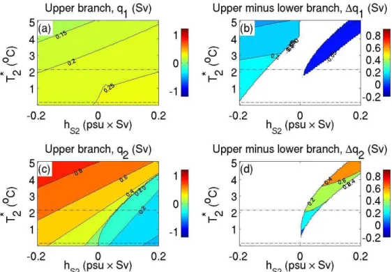
We have performed a similar analysis for Aegean-Ionian parameters, hS2
and T∗
2 (Fig. 6); the Adriatic-Ionian apparent temperature T1∗ is given
Ta-ble 1 and hS1 is assumed to be zero. As expected and with accordance with
the Aegean-Ionian interaction, with q1 ≈ 0.38 Sv (Fig. 6a). The
Aegean-Ionian flux, q2, is drastically affected by changes in hS2 and T
∗
2 (Fig. 6c,d).
For the pre-1990 conditions, the apparent temperature is T∗
2 ≈ 0.15 ◦C and
the Aegean-Ionian flux is almost zero when hS2 ≈ 0. Under cooling of 2 ◦C
over the Aegean (indicated by the dashed-dotted line in Fig. 6c) the flux may reach 0.8 Sv, depending on the surface salinity flux. This value is smaller than the observed value of 1 Sv and both alteration of air temperature and freshwater flux over the Aegean are required to achieve it. The bi-stability of thermally and salinity dominant states is achieved for positive surface salin-ity flux (i.e., fresher Aegean) and the extent of the bi-stabilsalin-ity region is larger
for greater apparent temperature T∗
2. Different values of T1∗ and hS1 lead to
different bi-stability regions.
Combinations of atmospheric changes over the Aegean and Adriatic basins may lead to the EMT following the scenarios discussed in this section. The above “mapping” does not meant to be realistic, but to demonstrate the model’s simulations fall within the range of the observed values.
4. Summary
We model the recent change in the deep water formation of the Eastern Mediterranean using a three box model. The boxes represent the Adriatic, Ionian, and Aegean seas. The equations governing the dynamics are nonlin-ear and may have four, two, or one stable states. We consider two cases: (i) the temperatures of the boxes are fixed and (ii) the temperatures of the boxes are variable. The Adriatic and Aegean boxes may each have, in principle, two states, one strong thermally dominant source of bottom water and the other with weak source. The thermally dominant source of the Aegean box is significantly stronger than that of the Adriatic.
We associated the EMT to switching between the different states of the system. Such transitions can occur, for example, due to rapid increase in salinity of the Aegean and rapid decrease in temperature over the Aegean. The Aegean sea became saltier after 1990 due to enhanced evaporation, river damming, and blocking of salty Levantine waters south of Crete due to three anticyclonic eddies that caused the salty Levantine water to pass north of Crete into the Aegean sea [3, 4]. Thus, one may expect the Aegean-Ionian flux state before 1990 to be salinity dominant with weak sinking in the Ionian be-cause of the positive salinity flux (leaving the Aegean pre-1990 relatively fresher compare to post-1990 Aegean state). Subsequently the Aegean water became
saltier, possibly causing a switch from the salinity dominant state to a tem-perature dominant state. This state is sensitive to changes in atmospheric temperature that may drastically change the strength of the deep water for-mation source over the Aegean. Indeed, cold winters were observed over the Aegean before and during the EMT [15, 16, 17].
The box model presented here does not include explicit parametrization of convection and wind. These two seem to be important for the under-standing of the EMT. It is possible to construct a box model of the Eastern Mediterranean that includes a simple form of these effects, similar to [33]. Such a model can be based on the Stommel box model [22], as done above, and on Winton [34, 35] relaxation oscillations deep convection box model.
The model proposed in this study highly simplifies the circulation of the Eastern Mediterranean. For example, a previous study [19] indicated the im-portance of the Levantine intermediate water on the thermohaline circulation of the Eastern Mediterranean; our model does not have surface and interme-diate boxes and thus does not explicitly model the Levantine intermeinterme-diate water. Including such boxes would be a logical next step.
The current model highly simplifies the complex 3D dynamical circulation of the Eastern Mediterranean. This simplicity allows us to capture and easily model the possible cause of the recent change in the Eastern Mediterranean. In addition our analysis indicates that large uncertainty is associated with the net moisture flux over the basins under consideration. Both the simplicity of the idealized box model and the large uncertainty of the data do not allow direct implementation of the box model to the Eastern Mediterranean. Thus, our results are only suggestive of the possibilities, and much more complex 3D models of the Eastern Mediterranean ocean are necessary to fully understand the complex changes in the Eastern Mediterranean thermohaline circulation. References
[1] W. Roether, B. Manca, B. Klein, D. Bregant, D. Georgopoulos, V. Beitzel, V. Kovacevic, A. Luchetta, Recent changes in eastern mediterranean deep waters, Science 271 (1996) 333–335.
[2] B. Klein, W. Roether, B. Manca, D. Bregant, V. Beitzel, V. Kovacevic, A. Luchetta, The large deep water transient in the eastern mediter-ranean, Deep Sea Res. 46 (1999) 371–414.
[3] P. Malanotte-Rizzoli, B. Manca, M. d’Alcala, A. Theocharis, S. Brenner, G. Budillon, E. Ozsoy, The Eastern Mediterranean in the 80s and in the 90s: the big transition in the intermediate and deep circulations, Dyn. Atmos. Oceans 29 (1999) 365–395.
[4] P. Malanotte-Rizzoli, B. B. Manca, S. Marullo, M. R. Alcala, W. Roether, A. Theocharis, A. Bergamasco, G. Budillon, E. San-sone, G. Civitarese, F. Conversano, I. Gertman, B. Hernt, N. Kress, S. Kioroglou, H. Kontoyannis, K. Nittis, B. Klein, A. Lascaratos, M. A. Latif, E. Ozsoy, A. R. Robinson, R. Santoleri, D. Viezzoli, V. Kovacevic, The Levantine Intermediate Water Experiment (LIWEX) Group: Lev-antine basinA laboratory for multiple water mass formation processes, J. Geophys. Res. 108 (C9) (2003) 8101.
[5] A. Lascaratos, W. Roether, K. Kittis, B. Klein, Recent changes in deep ocean formation and spreading in the eastern mediterranean sea, Prog. Oceanogr. 44 (1999) 5–36.
[6] P. Malanotte-Rizzoli, B. Manca, M. d’Alcala, A. Theocharis, A. Berga-masco, D. Bregant, G. Budillon, G. Civitarese, D. Georgopoulos, A. Michelato, E. Sansone, P. Scarazzato, E. Souvermezoglou, A synthe-sis of the Ionian sea hydrography circulation and water mass pathways during POEM-Phase I, Prog. Oceanogr. 39 (1997) 153–204.
[7] J. Nielsen, Hydrography of the mediterranean and adjacent waters, in: Report of the Danish Oceanographic Expedition 1908-1910 to the Mediterranean and Adjacent Waters, Vol. 1, 1912, pp. 72–191.
[8] R. Schlitzer, W. Roether, H. Oster, H. Junghans, M. Hausmann, H. Jo-hannsen, A. Michelaton, Chlorofluoromethane and oxygen in the eastern mediterranean, Deep Sea Res. 38 (1991) 1531–1551.
[9] G. Wust, On the vertical circulation of the Mediterranean Sea, J. Geo-phys. Res. 66 (1960) 3261–3271.
[10] P. Malanotte-Rizzoli, A. Hecht, Large-scale properties of the Eastern Mediterranean: a review, Oceanologica Acta 11 (1988) 323–335.
[11] W. Roether, R. Schlitzer, Eastern mediterranean deep water renewal on the basis of chlorofluoromethans and tritium, Dyn. Atmos. Oceans 15 (1991) 333–354.
[12] B. B. Manca, V. Kovacevic, M. Gacic, D. Viezzoli, Dense water forma-tion in the southern adriatic sea and spreading into the ionian sea in the period 1997–1999, J. Mar. Sys. 33-34 (2002) 133–154.
[13] A. Theocharis, B. Klein, K. Nittis, W. Roether, Evolution and status of the eastern mediterranean transient (1997–1999), J. Mar. Sys. 33-34 (2002) 91–116.
[14] V. Zervakis, D. Georgopoulos, P. Drakopoulos, The role of north aegean in triggering the recent eastern mediterranean climatic changes, J. Geo-phys. Res. 105 (2000) 26103–26116.
[15] H. Sur, E. ¨Ozsoy, U. ¨Unl¨uata, Simultaneous deep and intermediate depth convection in the northern levantine sea, winter 1992, Oceanologica Acta 16 (1993) 33–43.
[16] A. Theocharis, K. Nittis, H. Kontoyiannis, E. Papageorgiou, B. E., Cli-matic changes in the aegean influence the eastern mediterranean thermo-haline circulation (1986-1997), Geophys. Res. Lett. 26 (1999) 1617–1620. [17] S. A. Josey, Changes in the heat and freshwater forcing of the Eastern Mediterranean and their influence on deep water formation, J. Geophys. Res. in press.
[18] S. Samuel, K. Haines, S. Josey, P. Myers, Response of the mediterranean sea thermohaline circulation to observed changes in the winter wind stress field in the period 1993, J. Geophys. Res. - Oceans 104 (1999) 7771–7784.
[19] P. Wu, K. Haines, N. Pinardi, Toward an understanding of deep-water renewal in the eastern mediterranean, J. Phys. Oceanogr. 30 (2000) 443– 458.
[20] S. Marullo, R. Santoleri, P. Malanotte-Rizzoli, A. Bergamasco, The sea surface temperature field in the eastern mediterranean from advanced very high resolution radiometer (avhrr) data: Part ii. intermediate vari-ability, J. Mar. Sys. 20 (1999) 83–112.
[21] K. Stratford, K. Haines, Modelling changes in mediterranean thermo-haline circulation 1987-1995, J. Mar. Sys. 33 (2002) 51–62.
[22] H. Stommel, Thermohaline convection with two stable regimes of flow, Tellus 13 (1961) 224–230.
[23] S. Manabe, R. J. Stouffer, Two stable equilibria of a coupled ocean atmosphere model, J. Climate 1 (1988) 841–866.
[24] S. Manabe, R. J. Stouffer, Century-scale effects of increased atmospheric
CO2 on the ocean-atmosphere system, Nature 364 (1993) 215–218.
[25] E. Tziperman, K. Speer, A study of water mass transformation in the Mediterranean-Sea -analysis of climatological data and a simple 3-box model, Dynamics of Atmospheres and Oceans 21 (2-3) (1994) 53–82. [26] CLIVAMP-project, Final technical report of the European Union
con-tract Mast 3 (MAS3-CT95-0043): climate variability of the Mediter-ranean Paleo-circulation, Tech. rep. (1999).
[27] V. Artale, S. Calmanti, A. Sutera, Thermohaline circulation sensitivity to intermediate-level anomalies, Tellus 54A (2002) 159–174.
[28] P. H. Stone, Global scale climate processes and climate sensitivity, in: M. Marani, R. Rigon (Eds.), Environmental Dynamics Series V: Hy-drometeorology and Climatology, Istituto Veeto di Scienze, Lettere ed Arti, Venice, 1997, pp. 47–84.
[29] M. Nakamura, P. H. Stone, J. Marotzke, Destabilization of the thermo-haline circulation by atmospheric eddy transport, J. Climate 7 (1994) 1870–1882.
[30] P. Welander, Thermohaline effects in the ocean circulation and related simple models, in: D. L. T. Anderson, J. Willebrand (Eds.), Large-Scale Transport Processes in the Oceans and Atmosphere, NATO ASI series, Reidel, 1986.
[31] L. R. Haney, Surface boundary condition for ocean circulation models, J. Phys. Oceanogr. 1 (1971) 241–248.
[32] B. B. Manca, G. Budillon, P. Scarazzato, L. Ursella, Evolution of dy-namics in the eastern mediterranean affecting water mass structures and properties in the ionian and adriatic seas, J. Geophys. Res. 108 (C9) (2003) art. no. 8102 doi:10.1029/2002JC001664.
[33] Y. Ashkenazy, E. Tziperman, A wind-induced thermohaline circulation hysteresis and millennial variability regimes, J. Phys. Oceanogr. 37 (10) (2007) 2446–2457.
[34] M. Winton, Deep decoupling oscillations of the oceanic thermohaline circulation, in: W. R. Peltier (Ed.), Ice in the climate system, Vol. 12 of NATO ASI Series I: Global Environmental Change, Springer Verlag, 1993, pp. 417–432.
[35] M. Winton, E. S. Sarachik, Thermohaline oscillation induced by strong steady salinity forcing of ocean General Circulation Models., J. Phys. Oceanogr. 23 (1993) 1389–1410.
Table 1: The parameters for the 3-box model.
parameter short description value
Va,Vb,Vc volume of Adriatic, Ionian, and Aegean box 27,600, 640,000, 61,600 km3
Da,Db,Dc depth of Adriatic, Ionian, and Aegean box 0.23, 2, 0.385 km
k1,k2 Adriatic-Ionian, Aegean-Ionian flux constants 8.29 × 10⁸, 1.35 × 10⁹m3s−1
α thermal expansion coefficients 2.3 × 10⁻⁴(◦C)−1
β haline expansion coefficients 7.5 × 10⁻⁴(psu)−1
T∗
a, Tb∗, T1∗ Adriatic, Ionian, T1∗ = Tb∗− Ta∗ apparent temperature 14.51, 16.30, 1.79 oC
T∗
c,pre/post Aegean apparent temperature pre/post 1990 16.15, 14.15 oC
T∗
2,pre/post T2∗ = Tb∗− Tc∗ apparent temperature pre/post 1990 0.15, 2.15 oC
λ heat flux relaxation constant 8 × 10⁻⁶ m/s
Box a
Box c
Box b
q
1q
1H
S1H
TaBOX a
Adriatic
q
2q
2H
S2H
TcAegean
BOX c
H
S1H
TbH
S2BOX b
Ionian
Figure 1: Upper panel: The bathymetry map of the Eastern Mediterranean sea. The solid lines indicate the choice of the different boxes: Box a represents the Adriatic sea, Box b represents the Ionian sea, and Box c represents the Aegean sea. Lower panel: Illustration of the 3-box model of the Eastern Mediterranean sea. Note that positive fluxes (q1,2 >0) are associated with sinking in the Adriatic/Aegean boxes while negative fluxes (q1,2 <0) are
−1 0 1 2 q1 −2 −1 0 1 2 q2 (a) −1 0 1 2 q1 −2 −1 0 1 2 q2 (b)
Figure 2: (a) The basins of attraction of the four stable states (indicated by black circles). The gray dots indicate the semi-stable states and the white dot indicates the unstable state. The solid lines indicate the minima lines while the dashed lines indicate the maxima lines. This case resembles the case of weak and positive salinity flux forcing for which there are four stable states. The volumes of the boxes are: Va = 0.5, Vb = 10, and Vc = 1 in arbitrary units. (b) Same as (a) but for weak and negative salinity flux forcing for the Aegean (HS2 < 0). Here there are just two stable states (units are non-dimensional). The different gray shadings indicate the regions of attraction of the different stable fixed points.
(a) φ 0.1 0 q 1.2 1 0.8 0.6 0.4 0.2 0 -0.2 q1 0.8 0.6 0.4 0.2 0 -0.2 -0.4 (b) φ 0.1 0 -0.1 -0.2 q2 1.4 1.2 1 0.8 0.6 0.4 0.2 0 -0.2 q1 0.8 0.6 0.4 0.2 0 -0.2 -0.4 2 A B C D
Figure 3: A pseudo-potential φ(q1, q2) [Eq. (23)] of Fig. 2a,b for the case Vb ≫ Va,c. The figure illustrates that a small change in salinity flux may result in different stability, e.g., a small perturbation is needed to switch from the q2 <0 minima to other minima but the q2>0 minima are much more stable under perturbation. Under different choice of parameters the stability might be different. The capital letters in panel a indicate the location of minima (stable state) points. Among the possible pathways for the EMT are A→B→C and A→D→C.
−6
−4
−2
0
2
4
Temperature
T
1[
oC]
0
−4
−2
0
2
4
exact [Eq. (38)]
approx. [Eq. (39)]
(a)
(b)
Figure 4: (a) A comparison between the exact solution of Eq. (38) (solid black curve) and the approximated solution of Eq. (38) given by Eq. (39) (gray curve). The intersection between the solid curves and the horizontal dashed line are the possible solutions of Eqs. (38), (39). The right branch of the fourth order polynomial of Eq. (38) is approximated by a parabola given by Eq. (39). The arrow indicates the solution that we choose for Eq. (39); this solution is the closest to (and smaller than) the forcing apparent temperature. (b) In some cases the approximation of Eq. (39) does not have any real solutions since the polynomial is always larger than zero. In this case we choose T at the minimum of the parabola of Eq. (39) to be the solution—this minimum is indicated by the arrow.
Figure 5: (a) Flux, q1 (in Sv) between the Adriatic and Ionian boxes as a function of surface Adriatic-Ionian salinity flux, hs1 and the Adriatic-Ionian apparent temperature T1∗. The largest of two possible value of q1is depicted. (b) Same as (a) for the flux difference between the larger and smaller q1; only the region of bi-stability is plotted. (c) Same as (a) for Aegean-Ionian flux. (d) Same as (b) for the Aegean-Ionian flux. Note the small values in panels (c),(d), indicating that the Adriatic-Ionian interaction is almost decoupled from the Aegean-Ionian interaction. The horizontal dashed line indicates the Adriatic-Ionian apparent temperature, T∗
1, given in Table 1.
Figure 6: Same as Fig. 5 for the surface Aegean-Ionian salinity flux, hs2 and the Aegean-Ionian apparent temperature T∗
2. The horizontal dashed/dashed-dotted line indicates the Aegean-Ionian apparent temperature, T∗

![Figure 3: A pseudo-potential φ(q 1 , q 2 ) [Eq. (23)] of Fig. 2a,b for the case V b ≫ V a,c](https://thumb-eu.123doks.com/thumbv2/123doknet/14182258.476496/27.918.176.750.326.590/figure-pseudo-potential-φ-eq-fig-case-v.webp)