Assessing the long-term attractiveness of mining a commodity based on the structure of its industry

Assessing the long-term attractiveness of mining a commodity based on the

structure of its industry

by

Tanguy Marion

B.S. Advanced Sciences, L'Ecole Polytechnique, 2016

MSc. Economics and Strategy, L'Ecole Polytechnique, 2017

Submitted to the Institute for Data, Systems and Society in partial fulfillment of the

requirements for the degree of

MASTER OF SCIENCE IN TECHNOLOGY AND POLICY

AT THE

MASSACHUSETTS INSTITUTE OF TECHNOLOGY

JUNE 2019

@2019

Massachusetts Institute of Technology. All rights reserved.

Signature redacted

Signature of Author:

Tanguy Marion

Institute for Data, Systems and Society

Technology and Policy Program

May 9, 2019

Certified by:

Signature redacted

Richard Roth

Director, Materials Systems' Laboratory

Research Associate, Materials Systems' Laboratory

Thesis Supervisor

Accepted by:

Signature redacted

MASSACHUSElTSM NSTITUTE

Noelle Eckley Sellin

OF TECHNOLOGY

_{Director, Technology and Policy Program}

Associate Professor, Institute for Data, Systems and Society and

JUN

0Department

of Earth, Atmospheric and Planetary Sciences

LIBRARIES1

MITLibranes

77 Massachusetts Avenue Cambridge, MA 02139 http://libraries.mit.edu/ask

DISCLAIMER NOTICE

Due to the condition of the original material, there are unavoidable

flaws in this reproduction. We have made every effort possible to

provide you with the best copy available.

Thank you.

Some pages in the original document contain text

that runs off the edge of the page.

Assessing the long-term attractiveness of mining a commodity based on the

structure of its industry

By

Tanguy Marion

Submitted to the Institute for Data, Systems and Society in

partial fulfillment of the requirements for the degree of Masters

of Science in Technology and Policy

Abstract. Throughout this thesis, we sought to determine which forces drive commodity

attractiveness, and how a general framework could assess the attractiveness of mining

commodities. Attractiveness can be defined from multiple perspectives (investor, company,

policy-maker, mine workers, etc.), which lead to varying measures of attractiveness. The

scope of this thesis is limited to assessing attractiveness from an investor's perspectives,

wherein the key performance indicators (KPIs) for success are risk and return on investments

(ROI).

To this end, we have studied the structure of a mining industry with two concurrent

approaches. Both approaches aggregate 18 key drivers of ROI and risks, like demand growth,

the size of the reserves pool, or the share of state-owned enterprise. The first approach was

based on a microeconomics model of cost curve updates and led us to developing the Cost

curve model. The second one is based on industry expertise and on intuitive, logical and

transparent ways to account for the effects of different industry forces like barriers to entry,

market power or spikes likelihood on industry attractiveness. It led us to developing the

Decision tree model.

These two models are complementary: while the first is a rigorous framework that

relies on simplifying assumptions, the second relies on intuition and logic. Through this

complementarity the two models provide clear and aligned insights about (i) which key

combinations of key drivers are preeminent for attractiveness, (ii) how key drivers interact to

mitigate or enhance attractiveness, and (iii) how commodities can be screened at a high-level

in order to prioritize commodity investigation.

Table of Contents

ACKNOW LEDGM ENTS...8

BACKGROUND AND M OTIVATION...9

INTRODUCTION...10

1. INDUSTRY STRUCTURE DRIVERS OF ATTRACTIVENESS... 11

II. M ICROECONOM ICS AND BUSINESS ECONOM ICS THEORIES... 14

11.1. M ICROECONoMics THEORY ... 14

11.2. BUSINESS ECONOMICS THEORY...15

1I1. THE MICROECONOMICS AND BUSINESS ECONOMICS OF MINING ... 16

111.1. THE M ICROECONOMICS OF MINING ... 16

///.1.a. Com puting the supply loss ... 18

ll.1.b. Com puting the incentive curve capacity and costs ... 19

///1.1.c. Com puting the real dem and change ... 21

111.2. THE BUSINESS ECONOMICS OF MINING...22

111.2.a. Examples: Drivers interact in complex ways that shape commodity attractiveness...22

I.2.a.(i). Case study 1: Aluminium... 22

I Ce.2.a.(ii). Case study 2: Lithium ... 24

111.2.b. Fram ework: a logic tree approach to aggregating root drivers ... 25

II.2.b.(i). Forces that shape the change in supply... 27

Il.2.b.(ii) Forces that shape the change in demand ... 30

l1I.2.b.(iii) Forces that shape the uncertainty of supply ... 31

IV. DESIGN OF TWO MODELS BASED ON MICROECONOMICS AND BUSINESS ECONOMICS THEORIES...34

IV.1. DESIGN OF A MICROECONOMICS MODEL -A COST CURVE MODEL ... 34

IV.1.a Com puting the supply loss ... 34

IV.1.b. Com puting the shape and capacity of the incentive curve ... 38

IV.1.b.(i) Capacity of ICC...38

IV .1 .b .(ii) C o sts o f IC C ... 4 0 IV.1.c. Com puting the real dem and change ... 41

IV.1.d. Conclusion - Computing the next m argins... 42

IV.1.e. Next steps - M odel enhancem ent... 45

IV.2. DESIGN OF A BUSINESS ECONOMICS MODEL-A LOGIC TREE MODEL ... 46

IV.2.a. First step: utility functions of elem entary drivers... 46

IV.2.b. Second step: Aggregations of elementary drivers' scores... 48

V. RESULTS AND BENEFITS OF THE COST CURVE AND LOGIC TREE MODELS ... 51

V.1. RESULTS -COST CURVE MODEL ... 51

V.1.a. Regression tree analysis...52

V.1.b. Im pact of different drivers ... 57

V.2. RESULTS - LOGIC TREE M ODEL...59

V.3. - LOGIC TREE MODEL VS. COST CURVE MODEL ... 62

CONCLUSION ... 65

REFERENCES...66

APPENDIX ... 67

APPENDIX FOR SECTION IV...67

List of Figures

FIGURE 1: ILLUSTRATION - THE FIVE FORCES OF PORTER ... 15

FIGURE 2 ILLUSTRATION - COST CURVE, FOR A GIVEN COMMODITY ... 16

FIGURE 3 ILLUSTRATION -DISCRETE MODEL FOR THE OPERATING COST CURVE UPDATES...17

FIGURE 4 COM PUTING THE SUPPLY LOSS ... 18

FIGURE 5: COMPUTING THE INCENTIVE COST CURVE CAPACITY...19

FIGURE 6: COMPARISON OF ICC AND OCC, FOR COPPER...20

FIGURE 7: COM PUTING OF THE ICC DISTRIBUTION ... 21

FIGURE 8 : COMPUTING REAL DEMAND CHANGE ... 21

FIGURE 9 WORLDWIDE PRODUCTION OF ALUMINUM: 1999-2018... 22

FIGURE 10 : 2017 ALUMINIUM COST-CURVE ... 22

FIGURE 11 : CHINA AND REST OF WORLD PRODUCTION OF ALUMINIUM - 1999-2018 ... 23

FIGURE 12: LITHIUM AND COBALT PRICE, 2002-2018... 24

FIGURE 13 : FORCES THAT AFFECT LONG-TERM ROI... 25

FIGURE 14 : PRINCIPLE OF OUR SEMI-QUANTITATIVE, BOTTOM-UP APPROACH TO AGGREGATING ELEMENTARY DRIVERS...26

FIGURE 15 : BOTTOM-UP AGGREGATION OF DRIVERS' FLOW-CHART - BARRIERS TO ENTRY ... 27

FIGURE 16: BoTToM-UP AGGREGATION OF DRIVER'S FLOW-CHART- SPIKES LIKELIHOOD ... 28

FIGURE 17: ILLUSTRATION -COST CURVE FLATNESS IS A BARRIER TO EXIT ... 29

FIGURE 18: BoTToM-UP AGGREGATION OF DRIVER'S FLOW-CHART- MARKET POWER ... 29

FIGURE 19: BOTTOM-UP AGGREGATION OF DRIVER'S FLOW-CHART- DEMAND GAP...30

FIGURE 20: BoTToM-UP AGGREGATION OF DRIVER'S FLOW-CHART- UNCERTAINTY OF ROI FORECAST...31

FIGURE 21: ILLUSTRATION - UNCERTAINTY AND RISK AVERSION...33

FIGURE 22: M O DELING SUPPLY LOSS...34

FIGURE 23: COST CURVE MODEL - RATIONAL FOR FLATNESS SCORE ... 36

FIGURE 24: COST CURVE THEORY (ON THE LEFT) VS.COST CURVE MODEL (ON THE RIGHT) ... 37

FIGURE 25: DATA ANALYSIS FOR COPPER -ICC TO RESERVES RATIO...38

FIGURE 26: ILLUSTRATION -MARKET CYCLICALITY ... 42

FIGURE 27: COST CURVE MODEL - COMPUTING P90t + 1...43

FIGURE 28: COST CURVE MODEL - ADDING THE INCENTIVE AND OPERATING COST CURVES YIELDS A PIECEWISE LINEAR FUNCTION...44

FIGURE 29: : LOGIC TREE MODEL -UTILITY FUNCTION OF RESERVES ... 46

FIGURE 30: ILLUSTRATION -"BARRIERS AVERAGES" AGGREGATIONS...48

FIGURE 31: LOGIC TREE MODEL -SUMMARY OF AGGREGATION FUNCTIONS ... 50

FIGURE 32: COST CURVE MODEL - TOP OF THE DECISION TREE ... 52

FIGURE 33: COST CURVE MODEL - DECISION TREE - RIGHT BRANCH ... 55

FIGURE 34: COST CURVE MODEL - DECISION TREE - LEFT BRANCH (PART 1) ... 56

FIGURE 35: COST CURVE MODEL - DECISION TREE - LEFT BRANCH (PART 2) ... 56

FIGURE 36: COST CURVE MODEL - AVERAGE NEXT MARGINS (LEFT) AND MARGINS INCREASE (RIGHT) IN FUNCTION OF CURRENT M ARGINS AND INCENTIVE CAPACITY ... 57

FIGURE 37: COST CURVE MODEL - AVERAGE NEXT MARGINS (LEFT) AND MARGINS INCREASE (RIGHT) IN FUNCTION OF CAPITAL INTENSITY AND INCENTIVE CAPACITY ... 58

FIGURE 38: AVERAGE NEXT MARGINS (LEFT) AND MARGINS INCREASE (RIGHT) IN FUNCTION OF ORE BODY DEPLETION, DEMAND CA G R AND PRODUCTION COVER ... 58

FIGURE 39: SUMMARY OF 1 VS.1 PROEMINENCE OF INDIVIDUAL DRIVERS ... 59

FIGURE 40: LOGIC TREE MODEL- MARGINS SUSTAINABILITY SCORE FOR REAL WORLD COMMODITIES...60

FIGURE 41: LOGIC TREE MODEL -ROI SCORE FOR REAL WORLD COMMODITIES ... 60

FIGURE 42: LOGIC TREE MODEL - UNCERTAINTY SCORE FOR REAL WORLD COMMODITIES ... 61

FIGURE 43: LOGIC TREE MODEL - UNCERTAINTY SCORE FOR SYNTHETIC COMMODITIES OF TABLE 8 ... 62

FIGURE 44 : LOGIC TREE MODEL - ROI SCORE FOR SYNTHETIC COMMODITIES OF TABLE 8 ... 63

List of Tables

TABLE 1 ELEM ENTARY DRIVERS OF ROI AND RISK ... 11

TABLE 2:: COST CURVE MODEL - INTERPRETATION OF REGRESSION FACTORS...39

TABLE 3 : COST CURVE MODEL - RANGE AND PARAMETER SELECTED FOR THE FULL FACTORIAL SIMULATION OF SYNTHETIC CO M M O D ITIES ... 5 1 TABLE 4: COST CURVE MODEL - TEST SET METRICS FOR DECISION TREE FIT...52

TABLE 5 : COST CURVE MODEL - NEXT MARGINS FOR COMMODITIES WITH LOW TO HIGH INCENTIVE CAPACITY ... 53

TABLE 6 : COST CURVE MODEL - NEXT MARGINS FOR COMMODITIES WITH VERY LOW INCENTIVE CAPACITY - OPTION 1 ... 54

TABLE 7 : COST CURVE MODEL - NEXT MARGINS FOR COMMODITIES WITH VERY LOW INCENTIVE CAPACITY - OPTION 2...54

TABLE 8 : DESCRIPTION OF 10 SYNTHETIC COMMODITIES CHOSEN TO SPAN THE RANGE OF NEXT MARGINS PREDICTION ... 62

ACKNOWLEDGMENTS

Every person I met in Cambridge has taught me something over the course of these two years.

I am very grateful for having had the opportunity to put the shoes of an MIT graduate student.

The waltz of events, activities, debates and talks that happened on and off-campus facilitated some incredible learning experiences, whereby I became able to take a step back and better define my personal and professional aspirations.

Thank you very much to Dr. Rich Roth, who has invested greatly in me and in this thesis by providing insightful and indispensable feedback. Rich taught me to always keep in mind the high-level research goals, even when conducting hands-on granular-level analyses. He also empowered me to become always more resourceful when conducting research, by giving me an incredible amount of slack and autonomy when I needed it, and very relevant advice and directions when I needed it. Thank you also for being so broad-minded and permissive in allowing me the time to pursue my out-of-lab interests. Finally, thank you for our challenging, although too seldom, conversations on how to change the world.

Thank you very much to the Rio Tinto Economics team, which supported me financially and laid the foundation for this work. It was a real pleasure to work with them during the summer of 2018, and great learning experiences throughout these two years.

Thank you very much to the Materials System's Laboratory professional and student team. It's been a real pleasure to have the opportunity to work with Dr. Randy Kirchain, Dr. Michele Bustamante, Dr. Medhi Noori, and Frank Ryan throughout these two years. A special thank to Terra for her amazing support. Thank you to Bensu, Karan, Fengdi, Josh H., Joshua B., Hassam, Yasmina, Ehsam for creating a supportive working environment. Thank you also to Joel, whom I didn't have the pleasure to meet, but whose office I really appreciated.

Thank you very much also to the TPP administrative team. This incredible experience couldn't have happened without Barbara DeLaBarre, Edward Ballo, Dr. Frank Field and Dr. Noelle Sellin.

Thank you to the broskys for two formidable years of tolerating and enduring each other, and poutou to the poussinette.

Thank you so much to my parents, and to all those who helped me get here. Special thanks to the best elementary school teacher ever: Madame de Fougeroux, to Dr. Alain Camanes who taught me Maths, to Dr. Michael Foessel who gave me a strong interest for Philosophy, and to Denis Hirson who helped me with my applications and opened my mind on the appreciation of cultural differences.

BACKGROUND AND MOTIVATION

Socio-economic enterprises can be understood as utility maximization problems. The entity that conducts a given enterprise uses its assets in order to obtain results as good as possible, or in other words, in order to maximize its utility function.

The utility function depends on who is enterprising. This entity can be an individual, a company, a non-governmental organization or the government. Basic economic theory assumes companies maximize profit. On the other hand, policy makers may want to increase consumers' welfare by making sure that supply meets demand without causing demand shrinkage due to price increase. They may also want to increase society's welfare by taking into account externalities and labor's welfare, in addition to consumers' welfare.

Once the utility function is defined, the remaining question is to know how it can be maximized. For example, a financial investor can buy several financial products, which all boil down to some expected returns, and some expected level of risk. The investor knows her utility function (it is probably increasing in the returns and decreasing in the level of risk, and it otherwise depends on her personal preferences). Thus, in order to know how she can maximize her utility function; the investor has to assess the expected returns and risk-level.

Another example, perhaps more tangible than that of investment funds, is that of a company's board when it decides on its strategic plan and on its external growth prospects. Suppose that the board of SomeCompany Inc. pursues profit maximization only. How will they pursue this goal? They may plan to grow organically, to innovate, to diversify horizontally or vertically, to invest in operations, marketing or R&D, etc... They have limited assets and virtually unlimited prospects. Thus, they have to take a decision on how to optimize their assets in order to maximize profit. A straightforward way to do so is to rank the main prospects

by how attractive they are. Attractiveness is defined here as a combination of profitability,

feasibility, and uncertainty. An attractive enterprise is one that has a high utility for the entity conducting it, given the utility function it seeks to maximize.

Large mining companies stand somewhere between regular companies and investment funds. Where investor have a limited number of financial products to pick from, a mining company has an even more limited number of commodities to pick from. And while commodities can be understood as financial products, it is also true that a mining company can decide to vertically integrate and sell modified or manufactured products. Thus conceptualizing the attractiveness of mining commodities lies at the intersection of theoretical investment an business strategy.

While the fields of Financial Economics' and Business Strategyz provides various case studies and literature regarding the two examples above - namely, investment strategy and business strategy -, the literature doesn't provide an in-depth, systematic, approach to conceptualizing the attractiveness of mining commodities.

' W. Shar pe, Capital Asset Prices: A Theory of Market Equilibrium under Conditions of Risk

As outlined above, attractiveness of mining commodities can be defined from two main perspectives: (i) a financial investor's perspective and (ii) society's perspective. (i) assumes that the utility is a function of expected returns and risk and (ii) assumes it is a function of how efficiently the market works, and takes into account externalities (through, for instance sustainable supply chain management (SSCM)3_'4_{, corporate social responsibility (CSR)}5_' 6_{, and} socially responsible investment (SRI).

The scope of this study is limited to identifying and quantifying the drivers of attractiveness when it is defined as in (i): from a financial investor's perspective.

INTRODUCTION

As we outlined in the previous section, from an investor's perspective, the two main key performance indicators (KPI) are the return on investment (ROI), and the risk. Those two drivers are hard to quantify because of imperfect information. The ROl metric takes into account both the funds and effort required to invest. The risk measure has to be combined with the investor's "risk aversion". We will detail later the concept of risk aversion applied to mining. In a broad sense, a highly risk averse investor will favor a secure investment over a more uncertain one, even if the expected returns are lower.

Which driving forces make commodities attractive? What are the benefits of a general framework to assess mining commodities attractiveness?

A general framework has to be scalable across all commodities, without

in-depth commodity analysis. Thus, we need to be able to scale our assessment framework to any commodity with a reduced number of data inputs. To that end, we first identify the most important data inputs that are necessary to assess the attractiveness of a commodity, at a high level. Thus, we identify the elementary drivers that are required to assess any commodity's attractiveness level (I.). We then introduce the two economics theories (11.) that underpin two sound approaches to aggregating these drivers in a measure of attractiveness

(ll.). We then describe a possible implementation of each framework (IV.) and compare the

results obtained in each model (V.).

3 Helmut Asche, U Mainz, Industrial Policy Challenges in Resource-Rich Countries

4 Christoph Kolotzek, et al, _{A company-oriented modelfor the assessment of raw material supply risks,} environmental impact and social implications

s Zambia Institute for Policy Analysis & Research, In the Eye of a Storm: The impact of the economic slowdown on the labour market in Zambia.

6 Moritz, T., & Ejdemo, T., & S6d erholm, P., & WareI, L. The local employment impacts of mining: an econometric analysis of job multipliers in northern Sweden.

I

I.

Industry structure drivers of attractiveness

We are interested in assessing the long-term attractiveness of mining commodities. Thus, we need to predict risk and returns. Although it is hard to forecast these two KPI's directly, we notice that several factors drive them up or down. The first step was therefore to identify these drivers. This was done through literature review7, experts' interview, and iterative thinking when designing the models that we will present later on. The identified drivers and their definitions are summarized in Table 1, below.

Drivers

Current Margins (%)

Definition

Margins of the 25th percentile asset (P90/P25-1) Reserves (Or Production Cover) Reserves, as defined by USGS".

Production cover is the reserves, in years of current production

Asset concentration (%) Share of supply produced by the 10 largest mines

Geopolitical risk of reserves Ecountry Reserve Share - Country Risk

Intensity of regulations on Supply Qualitative - Scored between 0 and 1 by experts

Industry maturity Qualitative - Scored between 0 and 1 by experts

Technical complexity Qualitative - Scored between 0 and 1 by experts

Capital intensity CAPEX/P90 (Ratio of the capital expenditure of a typical project to the cost curve's 90% percentile's cost)

Geopolitical risk of supply E country Supply Share - Country Risk

SOE Concentration (%) Share of supply that is state-owned Vertical integration (%) Share of supply that is vertically integrated

Growth of demand (%) Base case, long-run forecast of the demand CAGR

Stocks (kt) Stocks, as defined by USGS9

Depletion (%) Share of yearly capacity decline due to ore grade loss

Risk of oligopoly stability disruption Qualitative - Scored between 0 and 1 by experts

10-year average of capacity utilization of oligopolist, weighted by share of Historical stability of oligopolist supply supply

Historical volatility of non-oligopolist

supply 10-year absolute growth of the share of supply produced by non-oligopolist lndustry concentration (%) Share of supply produced by the oligopoly

Substitution risk Qualitative - Scored between 0 and 1 by experts

Disruption risk Qualitative - Scored between 0 and 1 by experts

V1 Geopolitical risk of supply Same as in RO1 section

Intensity of regulations on Supply Same as in ROI section

SOE Concentration Same as in ROI section

Table 1 : Elementary drivers of RO and risk

Kanters, Supply risk assessment of major agricultural commodities; Spohn, Evaluating Market Attractiveness; Surujhal et al., Mining Company Strategy Evolution

8 USGS Mineral Commodity Summary 2018 - "Appendix C-Reserves and Resources"

I USGS Mineral Commodity Summary 2018

5

SC

0

Caa

We now succinctly expand on why we considered these drivers. Note that we considered many other possible inputs, that we did not keep as they were not as relevant as these one.

The long-run ROI of a commodity is defined as the long-run predicted margins for a good asset (2 5th percentile on the cost curve). 14 drivers affect the ROI.

- Current margins are a zero-degree approximation of long-run margin, they have

some indicating power. They also give the cost curve flatness (P25/P90 :Ratio of the cost curve's 25% percentile's cost to the 90% percentile's cost). Cost curve

flatness disincentivize non-economic firms to retire as the incurred loss is smaller

as the curve gets flatter.

- The amount of Reserves is also a driver of long-term profitability. This is easily seen as a shortage in reserves will induce a shortage in supply, or a higher cost of supply.

- Asset concentration is a proxy for the granularity of the industry, which translates

into high or low barriers to entry, and thereby into high or low margins.

- Geopolitical risk of reserves restricts the availability of deposits that could be

incentivized.

- Intensity of regulations on supply limits the ease with which new entrants can start

mining a commodity

- Technical complexity and Industry maturity limits the number of potential new

entrants. Only a few firms can manage to mine particularly complex ore bodies. On the other hand, when the industry is fairly new, like that of lithium, technological improvements are to be expected. In turn, these improvements might decrease the long-term technical complexity.

- Capital intensity also limits the number of potential new entrants.

- Geopolitical risk of supply generates price increase due to unforecastable capacity

shutdowns.

- SOE concentration disincentivize non-economic firms to retire, as the main goal of

SOE might go beyond mere profitability.

- Vertical integration disincentivize non-economic firms to retire, as the main goal

of vertically integrated firms might not be limited to the profitability of the mining segment of the value chain.

- Growth of demand increases consumption, and therefore the selling price (by

sliding towards the right-side of the cost curve)

- Stocks counterweight the growth of demand

- Depletion increases the need for new supply

In the situation where the market is oligopolistic, 4 additional drivers affect the ROI:

- Industry concentration is a proxy for how much market power the oligopoly firms

can exert

- Risk of oligopoly disruption, Historical volatility of non-oligopolist supply, and

Historical stability of oligopolist supply is a proxy for how much of this market

power is actually exerted.

0 Risk is a measure of how uncertain our forecast of ROI is. We will use the 16 drivers listed above (20 in the case of an oligopoly) to predict an expected value of ROI. Risk can be understood as a measure of the variance associated with that prediction. It depends on the supply and demand sides and results from the 5 following drivers:

- On the supply side, Geopolitical risk of supply, SOE concentration and the Intensity

of regulation on supply add uncertainty to the ROI forecast.

- On the demand side, Substitution and Disruption risk add uncertainty to the demand growth forecast, and in turn, to the ROI forecast.

These drivers are numerous, so they need to be aggregated to be readable. Margins and Risk are two complex functions of these drivers. Moreover, these drivers have a lot of interdependencies. For instance, high Growth of demand is of little use when barriers to entry, like the low level of Reserves or high Technical Complexity are very low (we will expand further on these considerations in section Ill., by providing real world case studies). Therefore, simple aggregations like a weighted average do not make sense and cannot inform decision-making. We develop two sound approaches to aggregating these drivers in the following sections.

II.

Microeconomics and business economics theories

In this section, we develop two approaches to aggregating the drivers identified in section I.. One based on microeconomics theory, and the other based on business-economics theory.

11.1. Microeconomics Theory

Fundamental principles:

Firms and consumers behave mostly in a rational way, based on imperfect information. They have given assets, which they allocate in order to optimize their utility functions. Their utility function can include several elements, like profit, market share or consumption.

The behaviors of individual economic entity are then aggregated to obtain supply and demand. Supply and demand are interdependent: a lack of supply will result in an increase in price (mostly because customers are more willing to pay, to obtain the scarcified good). An excess supply will result in a decrease in price (mostly because suppliers want to sell all their stocks, so they lower their prices to attract more customers). In turn, this change in price adjusts supply and demand, and the market converges to a steady state, which defines the long-run market price.

Takeaway - Firms' obiective:

The most basic theory assumes that firms are maximizing profit. Thus, their aim is to produce as much as possible, as long as the cost of production is below the market price. This implies that the market price is the marginal cost of production.

11.2. Business Economics Theory

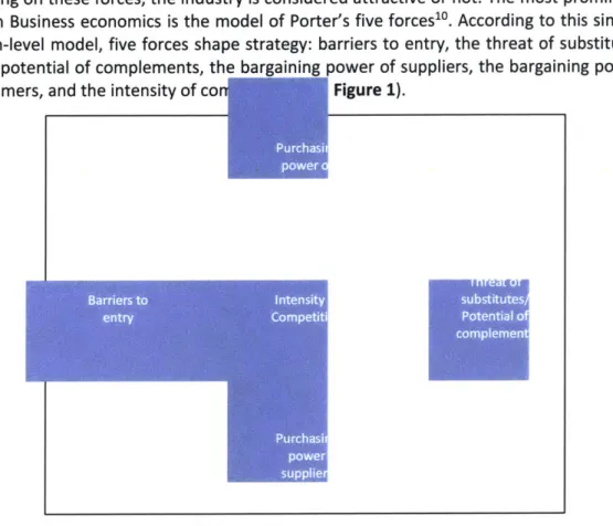
Industries are shaped by forces that interact and push the industry towards a stable state. Depending on these forces, the industry is considered attractive or not. The most prominent model in Business economics is the model of Porter's five forces'0. According to this simple and high-level model, five forces shape strategy: barriers to entry, the threat of substitutes and the potential of complements, the bargaining power of suppliers, the bargaining power of consumers, and the intensity of con M Figure 1).

Figure 1: Illustration -The five forces of Porter

For instance, high barriers to entry contribute to an industry's attractiveness, because if margins are high, the incumbents have more chances (i) to secure a large share of them on the long-term, and (ii) to maintain them on the long-term.

Similarly, high intensity of competition hurts the industry's attractiveness, because high competition usually drives the prices (and therefore, the margins) down.

Note: The literature bursts with such models", which all have interesting takeaways that we tried to incorporate in this study. We won't detail all such models as we did with Porter's five forces.

Takeaway - Firms' objective:

For a given industry, the force outlined above shape long-term attractiveness of this industry. Thus, depending on the current state, and on the investor's strengths and weaknesses, the investor will decide to enter or leave the market.

10 Porter, The five competitive forces that shape strategy

"1 SWOT analysis, PESTEL analysis, BCG matrix, https://www.mckinsey.com/business-functions/strategy-and- corporate-finance/our-insights/enduring-ideas-classic-mckinsey-frameworks-that-continue-to-inform-management-thinking

111.

The microeconomics and business economics of mining

In the previous section, we briefly summarized the two economics theories on which we will

base our approaches to aggregating the drivers identified in Section I.. In this section, we come

back to the more specific case of mining industry. We explain the ins and outs of both theories

in the specific case of the mining industry.

111.1. The Microeconomics of mining

In subsection 11.1. we derived from fundamental principles that the market price is the

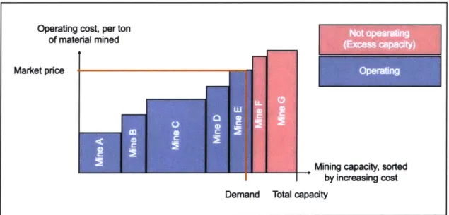
marginal cost of production. Figure 2 shows how this mechanism sets the price in practice. All

available mines are sorted by increasing cost. They each have a given capacity. The market

price is the operating cost of the last mine that has to operate in order to satisfy demand:

Mine E. If it were higher, Mine F could operate, and the market would be overflowed, so the

price would go down. If it were smaller, then Mine E would not operate, so there would be a

supply shortage, so the price would go up.

Operating cost, per ton

of material mined

Market price

___ ___ Mining capacity, sorted

by increasing cost Demand Total capacity

Figure 2: Illustration -Cost curve, for a given commodity

As explained in Section I., we want to predict the operating margins of a first-tier mine (i.e.

typically the mine that produces the

percentile of the supply: Mine B in Figure 2). The

operating margins of this mine are defined as:

Margins

=

Cost Unit cost * volume P25

where P90 denotes the price of the

percentile asset and corresponds to the market price

(in theory, the market price should correspond to the

00th

percentile assets, but in practice,

there is a lot of volatility for players at right the extremity of the cost curve).

Thus, in order to rank commodities by expected RO, we will leverage the drivers identified in

section

1.

to forecast the long-term P90 and P25. We will then be able to infer the next margins.

So far, we described mining cost curves as static. Forecasting the long-term margins entails of the 25th percentile asset requires to adopt a dynamic view of cost curves, wherein we predict the evolution of the operating cash cost curve, by taking into account the changes to the existing supply (supply loss due to depletion and mines closure), and the new supply coming from the incentive curve (i.e. the supply that is available but not operating). We do this with a discrete model that is illustrated in Figure 3.

Operadng cash cost curve

QitO

The operating cost curve shrinks

in capacity and increases in cost

Operating cash cost curve from time t

increase in cost (due to depletion) Capacity loss

depletion a

retirement)

e The mines from the operating and incentive

cost curve form the total available supply

~1

'I

Incenive (cash + discounted CAPEX) cost curve

CAPEX

* Given the new demand, all the economic

mines will operate

- The CAPEX (incentivization cost) is a sunk cost Operating cash cost curve p1Q4

Figure 3 : Illustration -Discrete Model for the operating cost curve updates

Excess ca ty Pio

t +.999

t+1

At time t, part of the supply is operating (top left quadrant), and part of it is excess capacity (top right quadrant).

With time, the operating parts shrinks in capacity due to retirement and depletion, and it increases in price due to depletion (middle left quadrant). Indeed, depletion consists in an ore grade loss, so with the same amount of effort and cost, a given mine will obtain less and less of the mineral as time passes by. Meanwhile, new deposits are prepared and can become operating if they are economical. These deposits add up to the excess capacity of time t, to form the incentive cost curve (middle right quadrant)

By merging the supply from the incentive curve and from the remainder of time t's operating curve, we obtain the total available supply at time t+1 (bottom left quadrant). Lastly, by using the demand in t+1,

Qit

t+1 (bottom right quadrant).

From there, we can easily find out P+ 1 _{and P2+1,}

which in turn will provide us the margins, using Equation (1).

To get there, we start from the information available at time t (top left and right quadrants), and we need to answer the following questions:

- _{What is the supply loss between t and t+1? Or in other words, how do we get} from the top left to the middle-left quadrant?

- _{What are the shape and capacity of the incentive cost curve Or in other words,} what is the middle right quadrant?

- What is

Qt+'?

_QtJ'

_Qt0?

Thus using microeconomics theory and this cost curve model, the next P90 and P25 can be inferred from Table 1: Elementary drivers of ROI and risk by following three steps:

- Computing the supply loss

- _{Computing the incentive curve capacity and cost distribution} - _{Computing the real demand change}

In the following development, we map Table 1's drivers to these three objectives.

Ill.1.a.

Computing the supply loss

Given our development so far, it is fair to assume that supply loss can come from one of two sources: ore grade loss, which decreases the capacity of a mine with time, and retirement (mine closure). We then break these two types of supply loss in elementary drivers from Table 1: Elementary drivers of RO and risk (in blue), and other cost curves metrics (in yellow) (see Figure 4).

Supply loss

Drivers from

18

Figure 4: Computing the supply loss

Loss from Loss from

retirement depletion

Economic Pu-0+I Operating

The loss from depletion is easily computed with the operating capacity and the depletion level. On the other hand, the loss from retirement comes from the next price and the barriers to exit (SOE concentration, vertical integration and cost curve flatness). As explained in section 11.1., it is a fundamental principle of microeconomics theory that a mine which produces at a cost higher than the market price should close. However, to take into account real-world factors, we consider three barriers to exit that might curb this behavior: SOE concentration, Vertical integration and Cost curve flatness (as this consideration was mostly motivated by the business economics approach, we will explain it in further details in section 111.2.b).

l11.1.b.

Computing the incentive curve capacity and costs

This step is one of the most perilous in our approach: there is no obvious way to infer precisely what the incentive curve is composed of.

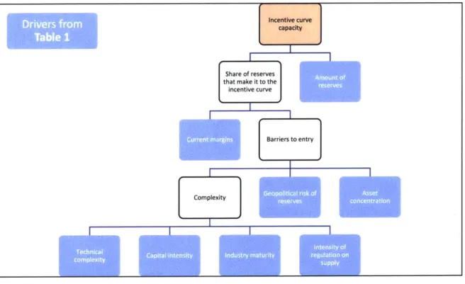
We reverse-engineer where the incentive mines come from. There is a given amount of reserves. Various reasons explain why all the reserves don't make it to the incentive curve. It might be that no company has decided to develop the required mining facilities because the enterprise is too uncertain, too hard, or unlikely to be profitable.

Quantifying the uncertainty related to deposits is outside the scope of this study. Therefore, we use barriers to entry and the current margins as a proxy to explain the share of deposits that become incentive mines between t and t+1 (see Figure 2).

Incentive curve capacity

Share of reserves that make it to the

incentive curve

C m iBarriers to entry

Cornplexity Gooiia iko

reere

Table 1

Figure 5: Computing the incentive cost curve capo

There are three barriers to entry, responsible for some deposits not making it to the incentive

capacity:

-1

sset

-

Complexity is an aggregate measure of Technical complexity, the Likelihood of a new

technology (for which we use Industry Maturity as a proxy), Capital intensity and

Intensity of regulation on supply. It accounts for the time it takes to set up operating

facilities, once the investment decision is made

-

Geopolitical risk of reserves is a weighted average of country risk and reserve shares

by country. It accounts for the inability to mine in certain areas due to corruption,

policies, political instability, and safety.

-

Asset concentration is measured by share of production corresponding to the 10

largest assets. It accounts for the difficulty for small players to penetrate the market.

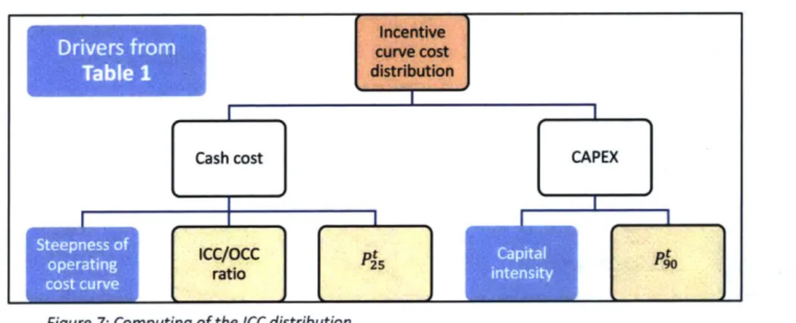
Now that we mapped Section L.'s drivers to the incentive capacity, we still have to infer the

cost distribution of the incentive curve. The discrete model for cost curve update explained at

the begin implies that the incentive cost curve is composed of the incentivization cost (or

CAPEX), which can be inferred from capital intensity and price, and of the cash cost. Inferring

the cash cost distribution is yet another perilous step.

Data analysis for copper indicates that it is fair to assume that the mine distribution of

operating cash cost (OCC) is approximately linear between Q25 and Q90 (see Figure 6).

Moreover, the incentive cash cost curve (ICCC) has approximately the same distribution as the

OCC

between Q25 and Q90. In other words, for any percentile p between 25 and 90,

P

Po'cc. This can be seen on the top graph of Figure 6.

2017 Copper. opetng mi (avg cost: 126.0 $ s. icentive mis favg cost: 123.0 $/0

017s d ostrgbutw n af 0pe5tng m1s1 -2.b..7Of00000 350 300 250

2017 Copper., oporaton minO (oog cost: 123.06/1)

IO

2017 Copper. onperating mine (avg cost: 122.0 $/U

- D.sArd.W-on f cetvin s

350

300

250

2D Vo-e(I$0120 50 70

~ISOr 6:Cmaio IC -,frcpen

Relying on these assumptions, we can assume two things: - In first approximation, cost curves are linear

- Since the ICC and OCC have the same distribution of costs (i.e. same extrema, median, percentiles...) it follows that the slope of the incentive curve is derived from the slope of the incentive curve by:

Slope1cc

Slopeocc

Hence, we have fully described how we can obtain the incentive curve cost distribution from

Section L.'s drivers and some exogenous assumptions. The results are summarized in

Incentive

Drivers from curve cost

Table 1 distribution

Cash cost

ICC/OcC p

Figure 7:- Computing of the ICC distribution

Note: the assumption leading to Equations 2 has been obtained based on copper data alone.

Studying further the relationship between ICC and

OCC

could improve this framework, but it

is out of the scope of this work.

lll.1.c.

Computing the real demand change

The last step to inferring the next P90 from Table 1: Elementary drivers of ROI and risk is to

obtain the new demand

Qt+.

This step is more straightforward, as we use Demand Growth as an input. We simply have to

adjust have to be careful about Stocks. The intuition is that when the price gets high, stocks

decrease because they are sold, so some of the demand is artificially filled by stocks, and

doesn't require new supply. Figure 8 sums up how we can compute the real demand change,

from elementary drivers.

Real demand change

Figure 8: Computing real demand change

CAPEX

111.2. The Business Economics of mining

In the section 111.2, we have introduced Business Economics theory. In this part, we first introduce the mechanisms by which elementary drivers shape the attractiveness of commodities, based on Business Economics theory. Then, we outline the complete framework through which individual drivers impact the attractiveness of commodities, and we argue why this framework is sensible.

111.2.a.

Examples: Drivers interact in complex ways that shape commodity

attractiveness

We first introduce how the elementary drivers defined in section 1. affect industry attractiveness, from a business theory perspective. For that, we try to find out what happened in the past, that made commodities (un)attractive today.

We will detail two interesting case studies here: Aluminium, and Lithium.

ll.2.a.(i). Case study

1:

Aluminium

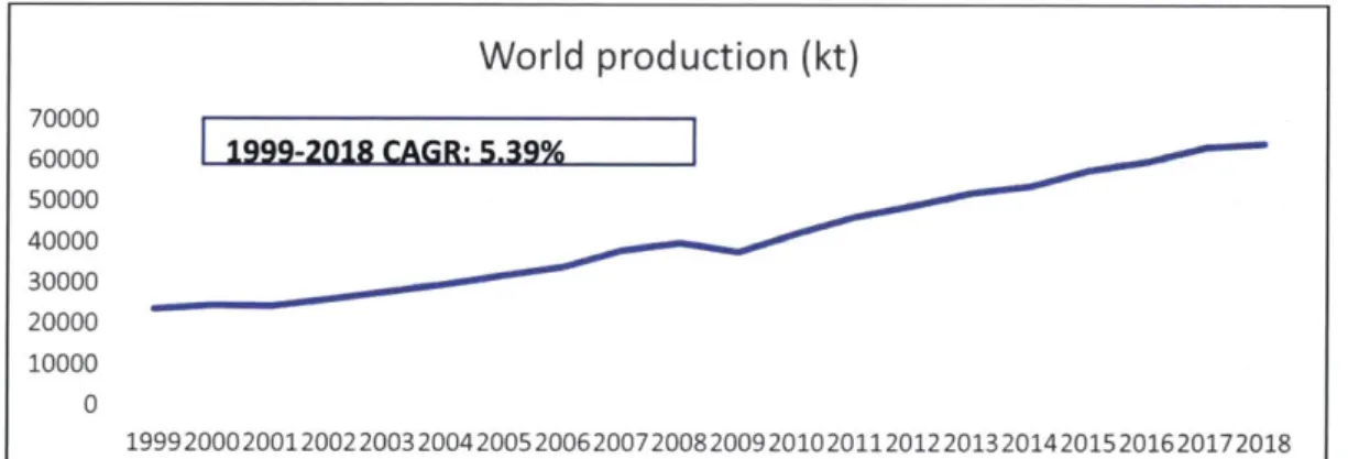
Aluminium demand grew steadily over the last 20 years, as illustrated on Figure 9 below. This growth was mainly driven by transport and construction.

World production (kt)

Figure 9: worldwide production of aluminum: 1999-201812

However, the aluminium industry is not attractive currently, as it is very competitive and has a very flat cost curve (9 = 1.31, see Figure 10 below).

P25 CRU BOC curve by smelter (2017) USDAl

2 500

Rest of world

21000

0 5000 10000 15000 20000 25000 30000 35000 40000 45000 50000 55000 60000 65000

Figure 10 : 2017 Aluminium cost-curve3

22

12 Source : www.world-aluminium.org

13 Source: https:/aluminiuminsider.com

Aluminium's growth has been almost showcased on Figure 11, below:

entirely captured by Chinese new entrants, as

China production vs. Rest of world production (kt)

I

Figure 11 : China and Rest of World Production of Aluminium - 1999-201814

So it is China's ability to build smelters at low cost and fast pace that absorbed all the demand

growth and prevented incumbents from extracting margins. What made it easy for China to

ramp up production in such a dramatic manner?

We can identify a few factors:

-

With over a 100 years of production cover there is no shortage of aluminium.

-

The country concentration of reserves being very low, aluminium is spread across the

world, and easy to access for Chinese smelters (The country with most reserves is Chile,

with 20%. And 1% of reserves represents 1 year of production).

-

As showcased by the very low asset concentration, small operations can be

competitive. In 2017, only 21% of the production was produced by the 10 biggest

assets. (this comes partly from the nature of the aluminium industry, which is not

directly a mining industry)

-

Capital intensity is very low for aluminium smelters, the CAPEX/P90 ratio being at 1.12

in 2017.

What these factors boil down to is that there are virtually no barriers to entry to the aluminium

industry. China's ability to build smelters at low cost and fast pace absorbs all the demand

growth, keeping the cost curve flat. Thus, high demand growth alone doesn't make a

commodity attractive unless barriers to entry are high.

60000 50000 40000 30000 20000 10000 0 14 Source: www.world-aluminium.org/ - -- - , -A

-A

1.2.a.(ii). Case study 2: Lithium

Between 2002 and 2018, the price of Lithium continuously increased, with a CAGR of 13.3%, while the price of cobalt peaked and dropped after the 2008 financial crisis, started recovering slowly in 2017 and dramatically in 2018 (see Figure 12).

Lithium -

Cobalt

-Price per metric tons (Inflation Adjusted) Price per metric tons (Inflation Adjusted)

$20000 $120000 $15 000 $100 000 $80 000 $10000 $60000 $5 000 $40 000 $20000 0 D00000r4r1 _ _ _ - I" _q r0 0~~ 0~~ 0000 r. - -r-1 r r-1r-15

Figure 12: Lithium and Cobalt price, 2002-2018

This results from the electric vehicles (EV) revolution and from the advent of other battery-intensive technologies like battery energy storage. This increase in demand should continue. According to McKinsey & Company's Lithium and Cobalt, a tale of two commodities, the demand will continue to increase at a very high pace for both commodities: +60% for cobalt and +300% for Lithium between 2017 and 2025.

The structure of the mining industries of these two commodities are very different, as Lithium is mainly a primary product, while cobalt is mainly mined as a by-product. Moreover, while both commodities are very geographically concentrated (with over 70% of production in the three top countries) Cobalt production is mainly based in areas of geopolitical instability, such as DRC.

Both commodities possibly face a very attractive future, with a considerable amount of uncertainty.

Uncertainty on the demand side:

- What will be the adoption rate of EVs? - Will new battery technologies emerge? And on the supply side:

- how will the barriers to entry evolve in the Lithium industry? (for now supply is very concentrated, but the resource base is enormous, so this could change in the future ; for now, mining Lithium is relatively complex, but the increased demand might lead to technological improvements...

Thus, the case of Lithium allows us to think of uncertainty. Uncertainty can come from the demand and supply sides, and the way to treat it will essentially depend on the investor's risk aversion (see next paragraph: subsection 111.2.b). It also makes us think of barriers to entry dynamically: Lithium seems to have high barriers to entry in 2017, with a high concentration of production and reserves, and with a high technical complexity. However, the resource base being very large, and the R&D for new mining technologies being thriving, one might expect a decrease of these barriers to entry in the near future.

24

111.2.b.

Framework: a logic tree approach to aggregating root drivers

So far, we have established that:

(I)

from a financial investor's perspective, two KPIs matter for attractiveness: returns on

investment (margins) and risk.

(ii)

These KPIs are driven by the features defined above (see section I.)

(iii)

These features interact in various ways that creates the conditions for attractiveness

or unattractiveness (see previous paragraph:

1ll.2.a.)

In this subsection, we explain at a high level the mechanisms by which these features cause

a positive or negative attractiveness. Later on, we will rigorously quantify these mechanisms

with mathematical functions.

The current margins of a given industry can evolve in two directions: they can shrink or

increase. As established in section I., several factors drive this change. These factors aggregate

in forces that shape the evolution of supply on the one hand and demand on the other hand

(see Figure 13 below).

The forces that shape the change in supply are barriers to entry, market power and spikes likelihood. The force that shape the change in demand is the demand gap.

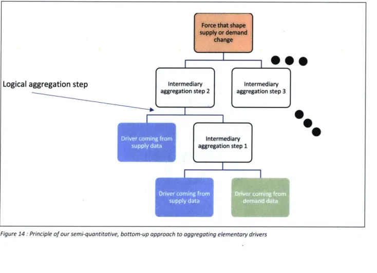
We quantify each force through a semi-quantitative, bottom-up approaches, from elementary drivers (see Figure 14 below). Each force is a function of given elementary drivers. In other words, elementary drivers interact in logical ways (that we formulate mathematically later on), that cause the forces outlined above to be strong or weak.

In the following development, we explain which elementary drivers determines which force, and how. The elementary drivers coming from supply data are colored in blue, those from demand data are colored in green, intermediary aggregation steps are colored in white.

Force that shape supply or demand

change

Logical aggregation step Intermediary Intermediary

aggregation step 2 aggregation step 3

Intermediary

suppl dataaggregation step 1

Figure 14 : Principle of our semi-quantitative, bottom-up approach to aggregating elementary drivers

ll.2.b.(i). Forces that shape the change in supply

Three forces shape the change in supply and the sustainability of margins, from a supply

perspective: barriers to entry, spikes likelihood and market power.

(I) Barriers to entry

Barriers to entry

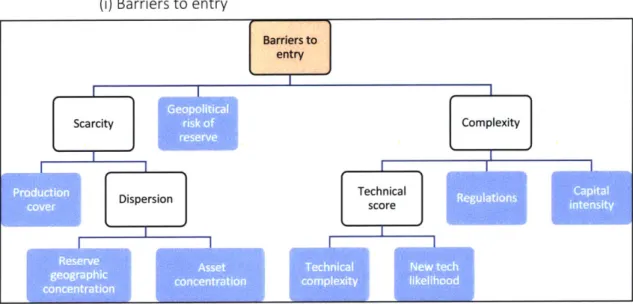
Figure 15: Bottom-up aggregation of drivers'flow-chart - Barriers to entry

There are three types of barriers to entry in the mining industry (see Figure 15 above):

- Scarcity: how hard is it for a firm to find available and economic deposits?

This barrier to entry depends purely on material's availability.

- Geopolitical risk of reserve: how safe are the deposits location? How easily may firms

obtain mining permits?

This barrier complements scarcity, it depends on the geopolitical climate of deposit locations

- Complexity: how hard is the material to mine? Can new entrants with little expertise

and technology enter in the industry?

This barrier complements the two formers, it depends mainly on the geology of deposits and on the ore extraction processes used for a given commodity. It also accounts for international regulations prompted complexity.

Scarcity and complexity barriers are further broken in elementary drivers:

- Scarcity:

Scarcity depends on the amount of material available (that we quantify by the production cover), and the degree of dispersion of this material. Huge deposits that are very concentrated in a given area results in a form of scarcity as fewer players will be able to operate them. On the other hand, even if a commodity is very evenly distributed across the world, if it is present in small quantity it is also scarce. In order to quantify dispersion, we use two measures of concentration: the geographic concentration of reserve, which accounts for the country dispersion of deposits, and asset concentration.

- Complexity: Capital intensity Complexity Technical _Regulations score 47 4 w tech likelihood Scarcity riko Dispersion

Mining complexity essentially comes from the geological aspect of mining. There is a technology barrier and a capital barrier. To measure the capital barrier, we use the Capital

intensity of a commodity. To measure the technical barrier, we take into account the current Technical complexity, and an adjustment variable for technical improvement (New tech likelihood), which helps better describing the long-term technical complexity of fast-growing

commodities, like lithium. On the other hand, for some commodities like uranium, Regulations add another complexity layer which we consider as a barrier.

(ii) Spikes likelihood

Spikes

likelihood

Barrieirs to

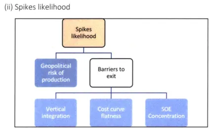
Figure 16: Bottom-up aggregation of driver's flow-chart - Spikes likelihood

Price spikes materialize in higher margins for top-tier players, and they have a particularly strong effect for some commodities, like copper.

They come from two effects (see Figure 16 above):

- Geopolitical risk of production: prices increase due to supply's inability to meet demand, because of sudden geopolitical crisis that entail capacity to close unpredictably.

- _{Barriers to exit: prices decrease due to suppliers not exiting the market despite being} uneconomic, because of barriers to exit.

Barriers to exit are further broken into three elementary drivers:

The three reasons that may incentivize a mine to continue operating despite being unprofitable are:

- Vertical integration: a given mine can be part of a larger business unit, which is

profitable other all. In our model, we focus on the margins extracted by the commodity suppliers. By being integrated downstream, company may capture a larger share of the margins across the value chain, and therefore still operate a mine which wouldn't be profitable if it were a stand-alone business unit.

- SOE concentration is another barrier to exit. State-owned firm might have

uneconomical goals. Actually, SOE concentration can be considered as a particular case of vertical integration: the mine is then seen as a micro element in the country's publicly owned economy. It's stand-alone profitability is not a main concern.

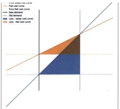
- Cost curve flatness is the last barrier to exit that we consider: the cost and hustle of

shutting down are more likely to outweigh profitability when the cost curve is flatter,

because a flat cost curve entails a smaller loss, and thus a smaller incentive to close.

This point is illustrated on Figure 17 below:

Flat cost curve Price flat cost curve - New demand

. Old demand m LoSs -steep cost curve - Loss -flat cost curve

Figure 17: Illustration -Cost curve flatness is a barrier to exit

(iii) Market power

So far, we discussed barrier to entry and spikes likelihood. The last item that contributes to

the change in supply and to building long-term margins, is the market power firms exert.

Market power

Oligopoly idsr

stability ocnrt

Riskof I Historical stablitystability

Market power is quantified through two factors (see Figure 18 above):

- Industry Concentration: Industry concentration is defined as the share of production detained by the oligopoly players. If there is an oligopoly, it quantifies how dominant its position is currently, and how strong an advantage the oligopoly firms have. A strong industry concentration means that the cost curve will be very convex, entailing high margins

- Oligopoly stability: how long lasting will the margins be? When there is an oligopoly mining a given commodity, the main players extract margins that depend mainly on their ability to maintain just enough room for small players to be profitable. The marginal cost of extraction sets the price, and these small players produce at higher cost, which guarantees high margin for the main players.

Ill.2.b.(ii) Forces that shape the change in demand

Demand gap

Figure 19: Bottom-up aggregation of driver's flow-chart - Demand gap

The demand gap essentially comes from demand growth, adjusted for structural effects from the supply side (see Figure 19 above). These structural effects are Depletion, and the volume of available stocks. For instance, a Depletion of x between years t and t+1 corresponds to a loss in production capacity of x. So it increases the demand gap by x.

The base case for demand risk forecasts (including substitution and disruption risks) is included in the demand growth input.

1ll.2.b.(iii)

Forces that shape the uncertainty of supply

So far, we described the forces that shape the return on investment (ROI). From a financial

investor's perspective, we also want to quantify risk. That is to say, the risk that supply or

demand don't behave in an economical way, or as forecasted. Or in other words, the risk that

the forecast of the ROI is off because players didn't behave as expected. In order to quantify

this risk, we proceed as we did with the attractiveness forces: from elementary drivers, up to

the uncertainty of ROI forecast.

In a first step, we assess how uncertain the ROI forecast is. Then, in a later step we combine

this measure with a score of risk aversion (which is dependent on the investor's profile), in

order to mitigate the next margin forecast.

(i) Uncertainty of ROI forecast

Uncertainty of ROl forecast

Demand risk Supply risk

Substtutin SO Reglatin on Geopoltical

Figure 20: Bottom-up aggregation of driver's flow-chart - Uncertainty of RO forecast

In order to assess the uncertainty of ROI forecast, we look at the demand and supply risks

(see Figure 20 above).

e

Supply side

Supply risk" comes from the non-economic behavior of firms. While it has been noted earlier

(1.b.) that this uncertainty can contribute to margin formation through an increased spikes

likelihood, we now consider this uncertainty from a risk aversion perspective.

Three main factors fuel the non-economic behavior of firms:

-

State-owned firms (SOEs) have non-economic incentives that may lead them to

produce at costs higher than prices

16 Christoph Helbig et al., Supply risks associated with lithium-ion battery materials

17 Erika Machacek, Constructing criticality by classification: Expert assessments of mineral raw materials

- Regulations on some commodities can prevent firms from entering and exiting the market at will, based only on economic profitability.

- Geopolitical risk can materialize in tensions that prevent firm from operating at full capacity

SOE concentration and regulations on supply have already been defined (see 1.b.). Geopolitical risks result from two items: geographic concentration and country risks. Thus, if a commodity is produced mainly in risky locations, it will have a high-risk score.

0 Demand side

Disruption risk and Substitution risk both factor in the demand growth forecast. They can constitute an opportunity or a threat for growth. In any case, they entail uncertainty, as stressed in the Lithium case study.

(ii) Risk aversion

As announced above, we combine this measure of supply uncertainty with the investor risk aversion's score. Depending on how risk averse the investor is, they will trust or distrust the margin score based on the uncertainty of supply score.

Our modeling of the investor's behavior is comparable to how people purchase apartments. When buying an apartment, the buyer has access to incomplete information only. They know whether it's a rather nice apartment or not, and they know the neighborhood in which the apartment is located. The information on the neighborhood can be very reliable, for instance it is clear that upper-east side is a nice neighborhood in Manhattan, or the information on the neighborhood can also be more speculative. For instance it wasn't clear a few years back that Soho or Chelsea would become such lively and nice places to live.

Knowing whether it's a nice apartment boils down to predicting the ROI for our investor. And the level of certainty the buyer has on the neighborhood corresponds to the degree of uncertainty of supply. If the buyer is risk averse, he will rather buy an apartment in a very certain neighborhood than in a speculative one. Even if the apartment of the certain neighborhood is not as nice. Similarly, a risk averse investor will favor less uncertain commodities although they might have a small predicted ROI, because he doesn't trust enough the information used to predict the ROI of uncertain commodities.

The different possible cases are summed up in Figure 21 below. The main takeaway is that a risk averse investor will most likely reject investment opportunities in highly uncertain commodities (bottom left quadrant).

High uncertainty and low aversion

- Supply uncertainty distribution Area of aversion

Area of comfort

Zone of uncertainty acception

-2 Hg n i r

High uncertainty and High aversion

Low uncertainty and low aversion

Zone of uncertainty acception

Low uncertainty and High aversion

-1

Figure 21: Illustration - Uncertainty and risk aversion

Zone of uncertainty acception

-2 -1 0

Zone of uncertainty acception I

I

0