MIT Joint Program on the
Science and Policy of Global Change
Biofuels, Climate Policy and the
European Vehicle Fleet
Xavier Gitiaux, Sergey Paltsev, John Reilly and Sebastian Rausch
Report No. 176 August 2009
The MIT Joint Program on the Science and Policy of Global Change is an organization for research, independent policy analysis, and public education in global environmental change. It seeks to provide leadership in understanding scientific, economic, and ecological aspects of this difficult issue, and combining them into policy assessments that serve the needs of ongoing national and international discussions. To this end, the Program brings together an interdisciplinary group from two established research centers at MIT: the Center for Global Change Science (CGCS) and the Center for Energy and Environmental Policy Research (CEEPR). These two centers bridge many key areas of the needed intellectual work, and additional essential areas are covered by other MIT departments, by collaboration with the Ecosystems Center of the Marine Biology Laboratory (MBL) at Woods Hole, and by short- and long-term visitors to the Program. The Program involves sponsorship and active participation by industry, government, and non-profit organizations.
To inform processes of policy development and implementation, climate change research needs to focus on improving the prediction of those variables that are most relevant to economic, social, and environmental effects. In turn, the greenhouse gas and atmospheric aerosol assumptions underlying climate analysis need to be related to the economic, technological, and political forces that drive emissions, and to the results of international agreements and mitigation. Further, assessments of possible societal and ecosystem impacts, and analysis of mitigation strategies, need to be based on realistic evaluation of the uncertainties of climate science.
This report is one of a series intended to communicate research results and improve public understanding of climate issues, thereby contributing to informed debate about the climate issue, the uncertainties, and the economic and social implications of policy alternatives. Titles in the Report Series to date are listed on the inside back cover.
Henry D. Jacoby and Ronald G. Prinn, Program Co-Directors
For more information, please contact the Joint Program Office
Postal Address: Joint Program on the Science and Policy of Global Change 77 Massachusetts Avenue
MIT E19-411
Cambridge MA 02139-4307 (USA) Location: 400 Main Street, Cambridge
Building E19, Room 411
Massachusetts Institute of Technology Access: Phone: +1(617) 253-7492
Fax: +1(617) 253-9845
E-mail: glo balcha nge@mi t.edu
Web site: htt p://gl obalch ange.m it.edu /
Biofuels, Climate Policy and the European Vehicle Fleet
Xavier Gitiaux†, Sergey Paltsev, John Reilly and Sebastian Rausch
Abstract
We examine the effect of biofuels mandates and climate policy on the European vehicle fleet, considering the prospects for diesel and gasoline vehicles. We use the MIT Emissions Prediction and Policy Analysis (EPPA) model, which is a general equilibrium model of the world economy. We expand this model by explicitly introducing current generation biofuels, by accounting for stock turnover of the vehicle fleets and by disaggregating gasoline and diesel cars. We find that biofuels mandates alone do not substantially change the share of diesel cars in the total fleet given the current structure of fuel taxes and tariffs in Europe that favors diesel vehicles. Jointly implemented changes in fiscal policy, however, can reverse the trend toward more diesel vehicles. We find that harmonizing fuel taxes reduces the welfare cost associated with renewable fuel policy and lowers the share of diesel vehicles in the total fleet to 21% by 2030 compared to 25% in 2010. We also find that eliminating tariffs on biofuel imports, which under the existing regime favor biodiesel and impede sugar ethanol imports, is welfare-enhancing and brings about further substantial reductions in CO2 emissions.
Contents
1. INTRODUCTION ... 1
2. TRENDS AND FORCES SHAPING THE DIESELVEHICLE MARKET ... 2
3. THE EPPA MODEL ... 6
3.1 First generation biofuels ... 6
3.2 The private transportation sector ... 12
3.2.1 Representation of the fleet turnover ... 13
3.2.3 Disagreggation of gasoline fleet and diesel fleet ... 14
3.2.3 Introducing E85 vehicles in EPPA ... 15
3.2 Implementing fuel standards in EPPA ... 16
3.4 Scenarios ... 17
4. RESULTS ... 17
4.1 The vehicle fleet ... 17
4.2 Welfare, emissions and trade impacts of fuel policies ... 20
5. SENSITIVITY ANALYSIS ... 25
6. CONCLUSION ... 27
7. REFERENCES ... 29
1. INTRODUCTION
Diesel vehicles have strongly entered the European car market especially in the last decade. They now account for over 50% of new vehicle registrations (ACEA, 2008). The likely reason for the strong penetration of diesel vehicles is a fuel tax structure that favors diesel. However, Europe is now seeing a number of new policy developments that could change the cost and relative prices of fuels. Of particular interest are new renewable fuels mandates. The recently proposed energy and climate package from the European Commission that would extend the Emission Trading Scheme (ETS) over the next twenty years also calls for an increase in
renewable fuels. According to the European Commission (2008) proposal to introduce biofuels mandates, 5.75% by 2010 and 10% beyond 2020 of renewable fuels (in volume terms) have to be blended into conventional fuels. This new initiative will interact with an existing tariff and tax structure that encourages domestic biofuel production and favors diesel imports. The overall outcome of proposed fuel policies on the diesel market is not immediately clear. At issue with the renewable fuels requirement are the cost and availability of biodiesel as currently produced biodiesel and ethanol use different plant feedstocks that lead to different cost and availability of the fuels. In particular, estimates (IEA, 2004) suggest that biodiesel produced from crops like rapeseed may be relatively expensive and its availability is limited compared with ethanol. However, diesel combustion is more efficient and the fuel is subject to lower excise taxes, possibly offsetting the higher cost of biodiesel. A comprehensive analysis, which takes into account these factors, is clearly necessary to assess whether proposed fuel policies will encourage further penetration of diesel vehicles or possibly reverse this trend.
In this paper we augment an existing global energy economic model to study how these various forces may reshape the structure of the European vehicle fleet over the next twenty years. We use the MIT Emissions Prediction and Policy Analysis (EPPA) model, which is a recursive dynamic computable general equilibrium (CGE) model of the world economy with international trade among regions (Paltsev et al., 2005). Given our interest, we start with the EPPA-ROIL version of the model that includes a disaggregation of oil production and refining sectors
(Choumert et al., 2006). The resolution required for our focus on the diesel vehicle market leads us to incorporate several improvements to the model: first, we add a representation of current technologies for biofuels production as earlier versions of the EPPA model contained explicitly only a second generation cellulosic technology; second, we disaggregate the private
transportation sector to model the competition between gasoline and diesel vehicles; third, we treat stock turnover of vehicles to allow a better representation of the inertia of the vehicle fleet as it affects the penetration of new technologies, and fourth, we represent an advanced vehicle that is capable of using up to 85% ethanol fuel blends.
The paper is organized as follows. Section 2 reviews recent trends and the main forces driving the European diesel market. In Section 3 we describe the EPPA-ROIL model and additions we have made for this study. Section 4 analyzes how interactions between fiscal policy and renewable fuel standards could change the structure of the European vehicle fleet. Section 5 investigates the sensitivity of these interactions to our modeling assumptions. In Section 6 we provide conclusions drawn from these simulations.
2. TRENDS AND FORCES SHAPING THE DIESEL VEHICLE MARKET
In 1997, diesel motorization represented 17.5% of the stock of passenger cars in Europe (EUROSTAT, 2008) and given that diesel vehicles were about 22% of new registrations that share was drifting only gradually upward. However, starting in 1998 the diesel share of new vehicle registrations began growing rapidly and by 2007 more than half of the new registrations in the European Union were diesel fueled vehicles (Figure 1).
The increase in diesel vehicles was likely driven by a combination of improved diesel technology and differences in relative fuel prices (inclusive of fuel taxes). Over the last decade European car manufacturers have been developing efficient and attractive diesel motors. In 1995, the consumption of fuel by a new diesel car averaged 6.6 L/100km1 against 7.9 L/100km for a new gasoline car (Figure 2). Both diesel and gasoline vehicles have improved so that by 2003 diesels consumed on average 5.7L/100 km while gasoline engines consume on average
7.2L/100km. The advantage of diesel vehicles is due in part to the fact that diesel injection engines are more efficient in terms of fuel consumption and that the energy content of diesel (35.6 MJ) is greater than that gasoline (32.2 MJ). In addition, manufacturers have succeeded in designing less noisy motors that emit fewer pollutants, making the newer diesel vehicles more attractive to consumers.
The higher efficiency comes at an additional cost for purchasing a diesel vehicle. Keefe et al. (2007) reports an average extra cost of around $2300. Green and Duleep (2004) report an average of $1750 for a small vehicle (2.0-2.5 L) and up to $2500 for a large vehicle (4.5-5.0 L). With fuel prices at 1997 level ($0.74/L for diesel and $0.96/L for gasoline at the gas station) and with a discount rate of 7%, the discounted fuel savings obtained with a diesel vehicle pay for the additional cost of the engines after 5 years. With higher fuel prices (such as in 2008 with
gasoline price peaking at $2.14/L and diesel price at $1.98/L in Europe) the payback period is much shorter (around 2 years).
Figure 1. Share of diesel sales in the new registrations of passenger cars in European
Union. Source: ACEA (2008).
0 10 20 30 40 50 60 S h a re ( % ) 1994 1996 1998 2000 2002 2004 2006 Year
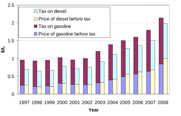
The relative price of gasoline and diesel at the pump is driven in part by the structure of fuel taxes in Europe that has favored diesel. For 1997 taxes on diesel were on average 31% lower than those on gasoline when calculated in terms of value per volume and 38% lower when calculated in terms of value per energy. The absolute difference in the tax rate on diesel and gasoline has remained a relatively stable over the last ten years, albeit with rising fuel prices the percentage difference has narrowed, as shown in Figure 3. The result has been lower prices at the pump for diesel than for gasoline when duties are accounted: in 1997 gasoline cost was $0.96/L whereas diesel cost was $0.74/L, in 2008 gasoline was $2.14/L and diesel was $1.98/L.
In addition to this tax structure, European fuel policy has called for increased use of biofuels in the transport fuel market. In 2005, the European Commission set the non binding target of 5.75% biofuels in transportation liquid fuels. In January 2008, in its proposal for Climate Action, the European Commission (CEC, 2008a) called for a 10% binding target for biofuels by 2020. Bolstered by such regulatory supports, biofuels have increased their share in the transport fuel market in recent years, reaching about 2.25% of the gasoline market and 3.5% of the diesel market (IEA, 2008) in volume terms. Whether these trends will continue depends in part on the cost of creating additional supply. In the longer term, technologies that convert lignocellulosic material to fuel have been a major focus of attention, but estimates suggest that those
technologies would not be developed to a level that would allow them to make much of a
contribution until the 2020 to 2030 period (Hamelinck, 2003). Nearer term prospects for biofuels thus requires more focus on the current technologies for biofuels production including ethanol from corn, wheat, sugarcane and sugar beet and the production of biodiesel from oil crops (soybean, rapeseed and palm fruit).
5 5.5 6 6.5 7 7.5 8 1995 1996 1997 1998 1999 2000 2001 2002 2003 Year L /1 0 0 k m Diesel motorization Gasoline motorization
Figure 2. Consumption of fuel to travel 100 km by motorization (European average).
The promotion of these alternative fuels interacts in Europe with a tariff structure that favors biodiesel imports over ethanol imports and, therefore, protects the domestic production of
ethanol. Jank et al. (2007) reports a high tariff of 0.192 €/L (63% ad-valorem equivalent in 2005) on non-denaturized ethanol imports and a lower tariff on biodiesel (6.5% ad-valorem equivalent). However prospects for biodiesel production in Europe are impeded on the one hand by its large requirement of agricultural feedstock and on the other hand by fuel standards that exclude the cheapest biodiesel for blended diesel/biodiesel products. The European fuel standards in EN 14214 (CEN, 2008) requires further processing of soy methyl ester to reduce its iodine content and of palm oil to increase its winter stability. In addition, fuel injection technologies face greater problems in using biodiesel.
Standards defining automotive gasoline and diesel allow a maximum content of 5% (in volume terms) of biofuels in conventional fuels (CEN, 2008). Standards that would allow for 10% of biofuels are under consideration. Higher blending rates, such as E85 (containing 85% of ethanol) would require flex fuel technology that has been developed only for gasoline vehicle (Intelligent Energy Europe, 2002), since the corrosiveness and the lack of stability of biodiesel prohibit a high blend rate (Bennett, 2007).
Figure 3. Prices before taxes and excise duties in Europe on diesel and gasoline. Prices and
excise duties are nominal prices estimated as an average of prices and duties in France, Germany, Italy and UK, weighted by their fuel consumption. Source: IEA (2008).
0 0.5 1 1.5 2 2.5 1997 1998 1999 2000 2001 2002 2003 2004 2005 2006 2007 2008 Year $ /L Tax on diesel
Price of diesel before tax Tax on gasoline
efficiency and effectiveness of such policies in a context of carbon dioxide mitigation. To
analyze how interactions among these various forces will reshape the European vehicle fleet over the next twenty years we augment the EPPA model to represent the cost of different vehicle and fuel choices.
3. THE EPPA MODEL
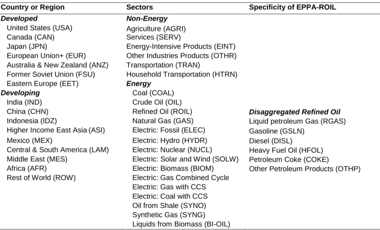
Our point of departure is the MIT Emissions Prediction and Policy Analysis (EPPA) model described in Paltsev et al. (2005). EPPA is a recursive-dynamic multi-regional computable general equilibrium (CGE) model of the world economy. The economic data from the GTAP dataset (Hertel, 1997; Dimaranan and McDougall, 2002) are aggregated into the 16 regions and 21 sectors shown in Table 1. The base year of the model is 1997. The EPPA model simulates the economy outputs recursively at 5-years intervals from 2000 to 2030. The model is written in GAMS software system and solved using MPSGE language (Rutherford, 1995).
Given our focus on transportation and fuel supply, we use a version of the EPPA model that relies on additional data to further disaggregate the GTAP data for transportation to include household transportation (Paltsev et al., 2004) and for the refining sector to include various types of fuels: gasoline, diesel, liquid petroleum products, heavy fuel oil, petroleum coke and other petroleum products (Choumert et al., 2006). The modifications we make to this version of the EPPA model include: representation of first generation biofuels (section 3.1); modeling of the private transportation sector that accounts for fleet turnover (section 3.2.1); disaggregation of the vehicle fleet to include separately gasoline and diesel vehicles (section 3.2.2); introduction a an advanced vehicle capable of using high blend of ethanol (section 3.2.3); and a structure for modeling renewable fuels standards (section 3.3).
3.1 First generation biofuels
The standard EPPA model includes a “second generation” cellulosic biofuels technology that in the long run and under climate policy would crowd out the current generation of biofuels (Reilly and Paltsev, 2007; Gurgel et al., 2008). The representation of current generation biofuels is, however, only implicit in the standard EPPA model to the extent that those fuels are contained in aggregate agricultural intermediate inputs into the fuel sector. As current biofuel technologies are more likely to contribute to meeting near term mandates and will hence play an important role in shaping the transition to second-generation biofuels, it is necessary to explicitly include these technologies in the model formulation.
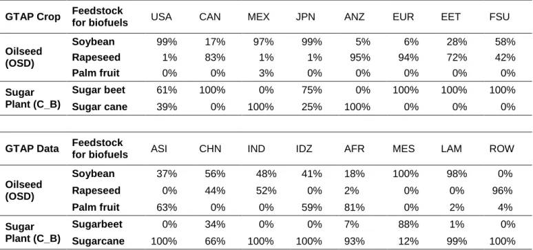
To include these fuels in the EPPA model we add production functions in the agricultural sector that represent production of the crops to be used as a biofuel feedstock. More specifically, we include biofuels based on sugar crops (sugar cane and sugar beet), grains (corn), wheat, and oilseed crops (rapeseed, soybean, palm oil). We utilize data from the GTAP input-output tables for the production of grain (GRO), wheat (WEA), oilseed (OSD) and sugar crops (C_B). We further disaggregate oilseeds into soybean, rapeseed and palm fruit, and sugar crops into sugar beet and sugar cane based on acreage shares of these crops in each EPPA region using FAO data (FAO, 2008) resulting in the shares shown in Table 2.
Table 1. Regions and Sectors in EPPA. Detail on the regional and sectoral composition is
provided in Paltsev et al. (2005), and for disaggregated refined oil sector in Choumert et al. (2006).
Country or Region Sectors Specificity of EPPA-ROIL
Developed Non-Energy
United States (USA) Agriculture (AGRI)
Canada (CAN) Services (SERV)
Japan (JPN) Energy-Intensive Products (EINT)
European Union+ (EUR) Other Industries Products (OTHR) Australia & New Zealand (ANZ) Transportation (TRAN)
Former Soviet Union (FSU) Household Transportation (HTRN)
Eastern Europe (EET) Energy
Developing Coal (COAL)
India (IND) Crude Oil (OIL)
China (CHN) Refined Oil (ROIL) Disaggregated Refined Oil
Indonesia (IDZ) Natural Gas (GAS) Liquid petroleum Gas (RGAS)
Higher Income East Asia(ASI) Electric: Fossil (ELEC) Gasoline (GSLN)
Mexico (MEX) Electric: Hydro (HYDR) Diesel (DISL)
Central & South America (LAM) Electric: Nuclear (NUCL) Heavy Fuel Oil (HFOL)
Middle East (MES) Electric: Solar and Wind (SOLW) Petroleum Coke (COKE)
Africa (AFR) Electric: Biomass (BIOM) Other Petroleum Products (OTHP)
Rest of World (ROW) Electric: Gas Combined Cycle
Electric: Gas with CCS Electric: Coal with CCS
Oil from Shale (SYNO)
Synthetic Gas (SYNG)
Liquids from Biomass (BI-OIL)
Production of biofuel crop j (j= grain, wheat, sugar cane, sugar beet, soybean, rapeseed, and
palm fruit) uses capital, labor, land, intermediate inputs supplied by various sectors of economy
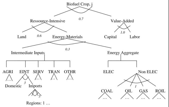
(agriculture, energy intensive industries, services, industrial transportation and other industries) and energy supplied by electricity, gas and refined oil. We derive the share of these inputs from the GTAP data. We represent crop production with nested CES functions shown in Figure 4. Land productivity is assumed to improve over time according to an exogenous trend (1% per year in developed regions and 1.5%-2% in Central and South America (LAM), Indonesia (IDZ), India (IND), China (CHN) and Africa (AFR)). Note, however, that land productivity (i.e. crop yields) varies endogenously over time and across the different scenarios as determined by relative price changes and by the elasticity of substitution between land and the energy-material bundle, and indirectly with the capital-labor bundle.
Table 2. Distribution of acreage between soybean, rapeseed and palm plant production and
between sugar cane and sugar beet in 1997.
GTAP Crop Feedstock
for biofuels USA CAN MEX JPN ANZ EUR EET FSU
Oilseed (OSD) Soybean 99% 17% 97% 99% 5% 6% 28% 58% Rapeseed 1% 83% 1% 1% 95% 94% 72% 42% Palm fruit 0% 0% 3% 0% 0% 0% 0% 0% Sugar Plant (C_B) Sugar beet 61% 100% 0% 75% 0% 100% 100% 100% Sugar cane 39% 0% 100% 25% 100% 0% 0% 0%
GTAP Data Feedstock
for biofuels ASI CHN IND IDZ AFR MES LAM ROW
Oilseed (OSD) Soybean 37% 56% 48% 41% 18% 100% 98% 0% Rapeseed 0% 44% 52% 0% 2% 0% 0% 96% Palm fruit 63% 0% 0% 59% 81% 0% 2% 4% Sugar Plant (C_B) Sugarbeet 0% 34% 0% 0% 7% 88% 1% 0% Sugarcane 100% 66% 100% 100% 93% 12% 99% 100%
Production of biofuel j use as an input biofuel crop j together with energy, intermediate industrial inputs (from OTHR, EINT, TRAN and SERV sectors of the EPPA model), and capital and labor, as shown in Figure 5(b). Because the relatively small amounts of biofuel production that occurred in the base year data are not explicitly represented in the GTAP dataset, we assume for our revised EPPA model that first generation biofuel technologies enter the market after 2000. For calibrating cost functions we base benchmark value shares on engineering analysis of their cost of production.2 For ethanol from grain, we follow the estimates for the cost of
production from Tiffany and Edman (2003) and Shapouri and Gallagher (2003). For ethanol from sugar crops, we use information available from USDA (2005) and IEA (2006). Finally, for biodiesel from oilseed, we use data from Hass et al. (2005) and Fortenbery (2005). From these studies we determine the cost components and the 2000 to 2005 average cost of production for corn ethanol in the United States, sugar cane ethanol in Latin America and biodiesel from soybean in the United States as provided in Figure 5(a). The cost of feedstock is between one quarter and one third of the total production cost of ethanol and 80% of the production cost of biodiesel.
2 The explicit technologies for production thus capture expansion of the industry beyond that amount implicitly
Figure 4. Production structure of biofuel crop sector j (j= grain, wheat, sugar cane, sugar
beet, soybean, rapeseed, and palm fruit). Vertical lines in the input nest signify a Leontief or fixed coefficient production structure where the elasticity of substitution is zero. Figures below the nests relate to the elasticity of substitution.
When adjusted to reflect the lower energy content of biofuels, costs of production range from $0.39/L for ethanol from sugar cane to $0.55/L for ethanol from corn and to $0.57/L for
biodiesel from soybean. We extend our cost estimates to other regions following the approach used in Gurgel et al. (2008). We assume that the conversion technology is the same in all regions but that the feedstock shares vary regionally according to differences in crop prices as reported by FAO (2008). For example, USA is the reference region for corn ethanol production in our approach, which means that we normalize input shares in the US to sum to one, while in other regions they sum to more or less than one depending on the relative price of corn, as provided in
Table 3. In the same fashion, Latin America is the reference region for sugarcane ethanol and
USA for soybean biodiesel. Where there was no crop price information from FAO (e.g. sugar cane in Canada) we assume that little or none of the crop is grown in that region and we then do not allow production of that fuel type in that region on basis that the country would need to import the crop and that transport costs would favor importing the fuel from countries that can produce the crop rather than the crop itself. We then apply a uniform mark-up multiplier across regions (1.3 for sugar cane ethanol, 1.9 for corn ethanol and 2.1 for soybean biodiesel) to the share parameters in the CES production function for all inputs. This ensures that the cost reflects
Biofuel Crop, j Ressource-Intensive Bundle Energy-Materials Bundle Land Intermediate Inputs Bundle
AGRI EINT SERV TRAN OTHR
Domestic Imports Value-Added Capital Labor Regions: 1 … n Energy Aggregate
ELEC Non ELEC
COAL OIL GAS ROIL
… … … … … … … … 0.7 0.6 0.3 1 3 5 1.0
the bottom up estimates of costs reported above for each biofuel relative to the price of gasoline or diesel in the reference region for the average 2000 to 2005 data.3
We extend cost structures from Figure 5(a) for wheat and sugar beet ethanol and rapeseed biodiesel produced in Europe, but we modify the relative weights between the crop and other inputs bundle to reflect the difference in feedstock prices. A comparison of the European, US and Brazilian prices for wheat, corn, sugar beet, sugar cane (FAO, 2008) and of rapeseed and soybean (USDA, 2008) allows us to estimate the 2000-2005 averaged cost of wheat ethanol at $0.65/L, sugar beet ethanol at $0.77/L and rapeseed biodiesel at $0.68/L. This estimate results in a mark-up (cost of production relative to refined oil) of 2.2 for wheat ethanol, 2.3 for rapeseed biodiesel and 2.6 for sugar beet ethanol. Following the approach described above, we extend these costs of production across all the EPPA regions in which these crops are produced. Table 3 provides the regionally specific data for biomass input shares. For example, for ethanol from corn the production shares in the US are 0.35 for capital input, 0.03 for labor input, 0.12 for energy, 0.11 for other industries (OTHR) inputs, and 0.39 for biomass feedstock input. As shown in Table 3, we use the same input shares across regions, except that for example, in Europe (EUR), the crop share is now 0.70 instead of 0.39 to reflect the relatively higher cost of corn. The same is true for other regions and technologies. The mark-up factor is then applied on top of all inputs.
The cost structure of biodiesel from palm oil and its mark-up factor (which is equal to 1.6) are evaluated with the same methodology by using the relative price of palm oil compared to soy oil (USDA, 2008). In addition, as noted previously in Section 2, biodiesel standards in Europe require products from soybean and palm oil to be further transformed before being injected in engines. Following Moser et al. (2007), we estimate the cost of these additional process steps at $0.05 per liter of biodiesel produced and therefore we raise the mark up for imports to Europe: from 1.6 to 1.8 for biodiesel produced from palm fruit and from 2.1 to 2.2 for biodiesel from soybean. Elasticities of substitution in Figure 5(b) are taken from the refined oil sector in Choumert et al., (2006).
3 EPPA follows a standard approach in CGE modeling whereby in the benchmark year all prices are normalized to
1.0 and outputs and inputs are denominated in dollars rather than in gallons, tons, or some other physical unit. We retain this basic normalization procedure for new technologies, appealing to cost data per physical unit of new technology relative to the cost of the technology it would replace to estimate the mark-up. This procedure assures consistency between the economic accounting of the model and supplementary physical accounting for physical units of energy, emissions, or land use.
(a)
(b)
Fuel j
Intermediate Inputs Bundle
EINT SERV TRAN OTHR
Domestic Import Biofuel crop j Capital Labor Regions: 1 … n … … … 0.2 3 5 Value added … 1.0
Figure 5. Structure for the production of biofuels. (a) Cost structure for biofuel production
(these estimations are established for ethanol from corn in USA, from sugarcane in Brazil and for biodiesel from soy oil in USA); (b) Structure of first generation biofuels
0% 20% 40% 60% 80% 100%
Percent of total cost of production
Grain Sugar plant Oilseed Fe ed st oc k Feedstock Chemicals Energy Other Capital
Table 3. Parameters used for the production function of first generation biofuels in EPPA:
mark-up and input shares (*** denotes absence of price information for the feedstock in the FAO dataset).
Input shares
Technology Mark-up Factor Capital Labor Crop Energy bundle OTHR
Ethanol from Corn 1.9 0.35 0.03 0.39 0.12 0.11 Wheat 2.2 0.29 0.02 0.49 0.10 0.10 Sugar Cane 1.3 0.47 0.16 0.26 0.05 0.06 Sugar Beet 2.6 0.27 0.09 0.57 0.02 0.05 Biodiesel from Rapeseed 2.3 0.05 0.03 0.84 0.02 0.06 Soybean 2.1 (2.2 for imports to EU) 0.06 0.03 0.81 0.02 0.08
Palm oil 1.6 (1.8 for
imports to EU) 0.07 0.04 0.77 0.02 0.10
Crop input shares for each technology (regionally specific)
USA CAN ME
X JPN ANZ EUR EET FSU
Ethanol from Corn 0.39 0.64 0.73 3.90 0.74 0.70 0.52 0.42 Wheat 0.38 0.33 0.47 4.41 0.47 0.49 0.42 0.54 Sugar Cane 0.58 *** 0.62 3.30 0.37 *** *** *** Sugar Beet 0.56 0.58 *** 1.84 *** 0.57 0.61 0.42 Biodiesel from Rapeseed 1.06 0.76 0.27 9.49 0.88 0.84 0.85 0.32 Soybean 0.81 0.84 0.91 10.61 0.95 0.83 0.66 0.49 Palm oil *** *** 0.79 *** *** *** *** *** ASI CH
N IND IDZ AFR
ME S LAM RO W Ethanol from Corn 0.66 0.58 0.60 0.69 0.86 1.07 0.52 1.47 Wheat 1.08 0.51 0.49 *** 0.92 1.16 0.56 1.57 Sugar Cane 0.40 *** 1.23 0.40 0.46 *** 0.26 0.73 Sugar Beet *** 0.71 *** *** 0.35 0.80 0.74 2.07 Biodiesel from Rapeseed *** 0.92 1.44 *** 1.45 *** 1.13 3.17 Soybean 1.09 1.13 0.93 1.28 1.60 4.85 0.80 2.26 Palm oil 0.75 0.73 *** 0.77 1.19 *** 1.19 3.34
3.2 The private transportation sector
We amend the existing transportation sector in the EPPA model in three ways: (1) We explicitly treat vehicle fleet turnover, (2) we disaggregate diesel and gasoline vehicles, and (3) we allow introduction of E85 vehicles. We adopt these modifications in the USA and EUR region only.
3.2.1 Representation of the fleet turnover
The previous approach in EPPA has been consistent with the National Income and Product Accounts (NIPA) practices that consider the private purchase of vehicles as a flow of current consumption. That representation underestimates inertia in the own-supplied transportation as vehicle fleets have a typical lifetime of 15 years. Our revised approach treats vehicles as capital goods that depreciate while providing a flow of services over their lifetime. NIPA data determine returns to capital as a residual of the value of the sales less intermediate inputs and labor cost. By assuming a rate of return and a depreciation rate, it is then possible to impute the level of the capital. The private transportation sector provides a flow of services that is not directly marketed and thus, there is no directly comparable data on the gross value of the transportation services from which intermediate inputs can be subtracted.
We use a cost approach that estimates the value of private transportation services as the sum of the costs incurred by the owner, including capital cost and operating costs. We first evaluate the value of the stock of cars from historical sales and then, impute the rental value of the stock of cars assuming an appropriate depreciation rate δ and a rate of return R on capital. The rental value of capital is derived from a Jorgenson-type estimation of R, which is the sum of the depreciation rate and a rate of interest r:
R r .
We use a constant depreciation rate that accounts for the average life of a vehicle. The European Association of Automobile Manufacturers (ACEA, 2006) provides us with the distribution of 2006 car stock by age in the EU15 and with new cars registrations since 1979. The lifetime function deduced from these data characterizes the European stock of cars with a mean lifetime of about 15 years and an average age of about 8 years. An exponential fit of this function produces a depreciation rate of about 8%. In addition, we assume that the real rate of interest is 5% to be consistent with the treatment of other industrial assets in EPPA.
We represent the vehicle fleet as a vintaged capital stock, similar to the representation of industrial sectors in EPPA (see Paltsev et al., 2005). The total stock of vehicles at time T is:
v v T n T T KC KC KC
where the superscript n denotes new vehicles, and v=1,...,4 are the multiple vintages of pre-existing vehicles. For each vintage:
1 1 ) 1 ( Tv v T KC KC
where v = 0 are the new vehicles from the previous period, and because we carry only 4 vintages there is 100% depreciation of the oldest vintage v=4. Each vintage is represented as a fixed coefficient production function. Purchasers of vehicles can choose the fuel efficiency and other characteristics of new vehicle but once they are part of the fleet these characteristics are frozen. For other industrial sectors we include a share, θ, of new capital that is vintaged, to represent the
We follow the approach of Paltsev et al. (2004) where own-supplied transportation (OWNTRN) uses inputs from the other industries (purchase of cars), from the services sector (maintenance, insurance) and from the refinery sector (see Table 4). Because we now consider the vehicle fleet as a capital stock we remove from household current consumption the payment for new cars and for used cars. The former is now added to the total of capital goods. Its value is derived from the value of private consumption of the “manufacture of motor vehicles” sector in the GTAP dataset. The purchase of used cars is removed from the account for the flow of private transportation services because in our approach this transaction does not modify the total amount of capital endowed to the final consumer. Household expenditure surveys on transportation suggest that used vehicle purchases account for about 14% of the total expenditures for the private transportation (BEA, 2008). As noted in Paltsev et al. (2005), services inputs in the own-supplied transportation have a large share because they include not only financial services, maintenance, insurance but also services related to the distribution of fuel.
Table 4. Input shares in the private transportation sector by type of engine for new
registrations in the benchmark year.
FUEL OTHR SERV
Private transport sector
Paltsev et al. (2004)
USA 0.080 0.220 0.700
EUR 0.240 0.260 0.500
FUEL CAPITAL SERV
Private transportation sector net of taxes
Gasoline vehicle
USA 0.127 0.131 0.742
EUR 0.105 0.241 0.655
Diesel vehicle USA 0.083 0.175 0.742
EUR 0.093 0.252 0.655
Private transportation sector with fuel taxes
Gasoline vehicle
USA 0.127 0.131 0.742
EUR 0.425 0.137 0.438
Diesel vehicle USA 0.083 0.175 0.742
EUR 0.270 0.292 0.438
3.2.3 Disagreggation of gasoline fleet and diesel fleet
Information derived from EIA (1994) for USA, from the European Commission (CEC, 2008b), and from Bensaid (2005) provide us with an estimate of the stock and the sales of diesel passenger cars in 1997. Average on-road fuel use per unit of distance (ACEA, 2003) allows us to estimate the physical share of diesel in the total consumption of fuel for private transportation in 1997. We multiply this share by estimates of relative fuel prices (IEA, 1998) and deduce the value of diesel expenditure as a share of total expenditures on refined oil products in the private transportation sector. With these typical fuel economy numbers we also evaluate the total miles driven in 1997 by diesel and gasoline fleet. Since we assume that one mile driven with a diesel car provides the same mobility service as one mile driven with a gasoline car, the share of diesel private transportation in the total flow of private transportation services is equal to the share of miles driven by diesel engines. Based on this hypothesis, we split the value of the private
transportation output (OWNTRN) between diesel (OWNTRNdisl) and gasoline (OWNTRNgsln) technology.
The higher efficiency of diesel combustion implies a higher input share for the services-capital bundle in the diesel own-supplied transportation sector. This is not surprising, as we have noticed in Section 2 that better efficiency comes at an additional cost for purchasing a diesel vehicle. As we assume that the share of services input is the same in both technologies, we can fully determine the structure of the diesel and gasoline private transportation, as provided in Table 4. From shares net of taxes, we can deduce that in Europe, the rental value for a new diesel vehicle is $100/year more expensive than for a new gasoline vehicle, meaning that given an interest rate at 5% and a depreciation rate at 8%, the purchase of diesel engine is $600 more expensive than the purchase of gasoline engine. This number has to be compared with
discounted savings of $500 that are obtained due to the better efficiency of diesel engine with fuels at 0.25/L (exclusive of taxes) in 1997.
GTAP data do not differentiate taxes on diesel and gasoline. We use data from IEA (2008a), illustrated previously in Figure 3, to determine the ad-valorem tax on gasoline in the benchmark year and to establish revenue raised by these excise duties. The excise duty on diesel is then adjusted to keep the revenue from fuel taxes equal to the revenue accounted in GTAP in 1997.
The elasticity of substitution used in these production sectors are derived from the survey of econometrics studies in Paltsev et al. (2004), which suggests estimates for short run elasticities between fuel and other inputs in the range of 0.2-0.5 and for long run elasticities in the range of 0.6-0.8. For the transportation services provided by new vehicles, we use the long run elasticity of substitution that is assumed to capture the ability to respond to higher fuel prices by
purchasing more efficient vehicles. With the vintaging structure the aggregate short run elasticity will reflect a weighted average of old vintages with a zero substitution elasticity and the new vintage with the high elasticity. Persistently high prices will then gradually lead to a vehicle fleet with greater efficiency. Vintaging captures structurally the observed difference between short and long run elasticities.
3.2.3 Introducing E85 vehicles in EPPA
Blending more than 10% of biofuels into conventional fuels may damage vehicles that are not designed to utilize them. Thus, fuel standards limit the blending percentage. In the U.S. the 10% limit is often referred to as the blending wall, because it would limit biofuel use absent vehicles that could use a greater percentage. In Brazil, flex-fuel vehicles that can run on any mix of ethanol and gasoline are popular. They accounted for 84% of new sales at the beginning of 2009 according to ANFAVEA (2009). In the United States E85 vehicles that can run on blends of up to 85% ethanol have been introduced in response to fuel-economy compliance credits offered by the Department of Transportation since 2001 (NHTSA, 2001). In 2007, almost 5% of the 17 million new light-duty vehicles sold in the U.S. were E85 vehicles.
However, modifications (including a stainless fuel tank and a special sensor to adjust engine spark timing) add an estimated $200 to the vehicle cost (Keefe et al., 2007). That extra cost translates to a mark-up of 1.015 on the capital input share in the E85 fleet production function. The main advantage of including E85 vehicles explicitly is that the vintaging of the vehicle fleet limits the use of ethanol based on the 10% blending wall on conventional vehicles and the growth of the stock of E85 vehicles available.
There are also additional costs associated with distribution of E85 fuel. For example, adding an E85 pump at a service station is estimated to cost approximately $200,000 (Keefe et al., 2007). IEA (2006) estimates that the total infrastructure changes needed for the transport, storage and distribution of E85 add about $0.06/gal to the price of ethanol. We add this additional cost for selling E85 in the services input in the production block of E85.
3.2 Implementing fuel standards in EPPA
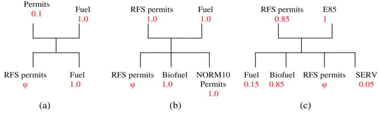
There are at least a couple of ways one could represent fuel standards in the EPPA model. One approach would be to introduce a quantity constraint in the GAMS-MPSGE algorithm used in the EPPA model. A second approach is to create a system of permits. We use the permit approach. We implement the permit approach as follows: Firms that produce one unit of
renewable fuel receive one Renewable Fuel Standards (RFS) permit. Every unit of conventional fuel or of its perfect substitute requires the surrender of a quantity of RFS permits to meet the renewable fuel mandate, specified as a share, φ, of total fuel. The conventional refiners must acquire permits from the renewable fuel producers. This approach captures the redistribution of funds between conventional refiners and biofuels producers, as fuel sellers must pay a premium (the permit price) to renewable fuel producers.
To capture the 10% blending wall and E85 fuel production we introduce another set of permits (which we refer to as NORM10 permits) and two blending processes that complement the conventional refinery sector. The conventional refinery produces conventional fuel. The 10% blending process is a combination of conventional refinery that is mandated to surrender φ RFS permits and of biofuels industry that uses as inputs biofuels and NORM10 permits and produces RFS permits and a perfect substitute for conventional fuel. In this way we allow biofuel
production only up to the amount of NORM10 permits available. The E85 blending process is a fixed coefficient production function blending 85% biofuels and 15% conventional fuel.
Conventional refineries produce 0.1 NORM10 permits for every unit of fuel produced. This ensures that the total number of NORM10 permits is only 10% of total fuel production. Use of E85 is more expensive because of the extra distribution costs and higher vehicle costs. Thus, a fuel mandate of φ < 10% can be met using the 10% blending process up to that level needed to meet the target, and even if biofuels are economic without the mandate, they are limited to not more than 10% unless they overcome extra cost of using E85. A fuel mandate of φ > 10% requires use of the E85 blending process, and at high enough φ E85 will crowd out the 10% blending process. The structure of the permit approach is represented in Figure 6.
3.4 Scenarios
We use the extended version of the EPPA model to implement four alternative scenarios in order to investigate interactions between fuel policy in the European transportation sector and the prospect for diesel vehicles. The first scenario is the no climate policy reference or business-as-usual (BAU), with the current tax and tariffs structure described in Section 2. The second scenario (MAND) simulates the European Commission (2008) proposal to introduce mandates on renewable fuels: 5.75% by 2010 and 10% beyond 2020 (in volume terms) have to be blended into conventional fuels. The last two scenarios include the biofuel requirements of the MAND scenario but vary the tax and tariff policy. The MAND_TARIFF scenario removes tariffs on ethanol and biodiesel imports. The MAND_TAX scenario replaces the differentiated fuel taxes by a uniform ad-valorem rate on all liquid fuels at the gas station which is set at a level to keep revenues constant at the BAU level. In fact, to ensure comparability with the reference case, we endogenize fuel taxes in the MAND and MAND_TARIFF scenarios to keep total tax and tariff revenues constant at the BAU level. The revenue neutrality requirement is important because we want to compare welfare cost implications across scenarios, and without a revenue neutrality assumption the welfare results would depend arbitrarily on where the tax or tariff rate is set. Both tax and tariff policies are implemented in 2010 jointly with renewable initiatives.
4. RESULTS
Our results focus on the relative penetration of diesel and gasoline vehicles, fuel prices, the composition and sources of fuels, welfare effects of the policies, CO2 emissions, and trade in
fuels.
4.1 The vehicle fleet
RFS permits φ Fuel 1.0 Fuel 1.0 RFS permits 1.0 NORM10 Permits 0.1 E85 1 Fuel 1.0 RFS permits φ 1.0 Biofuel NORM10 Permits 1.0 RFS permits φ Biofuel 0.85 Fuel 0.15 RFS permits 0.85 SERV 0.05 (a) (b) (c)
Figure 6. Implementation of renewable fuels standards in EPPA. (a) Production function of
conventional fuel; (b) Production function of blending of biofuels into conventional products up to 10%; (c) Production function of E85. Vertical lines in the input nest signify a Leontief or fixed coefficient production structure where the elasticity of
substitution is zero. Figures below the inputs name are the value of inputs shares. The φ is the renewable fuel standard.
the price of diesel - $5.63/gal by 2030- at the gas station below the price of gasoline - $6.30/gal by 2030 (Table 5) and by the general increase in oil prices that favors the most efficient
motorization. The share of diesel vehicles drifts upward gradually due to sales of new diesel cars that stabilize around 33-35% of the new registrations after 2020. These numbers are lower than the current sales of diesel vehicles in Europe (up to 50%) because the endogenously determined oil price in the model reaches $50/bbl by 2030, below those levels through 2008 that were strongly driving the diesel trend in Europe.
A factor behind the gradual leveling off of the diesel share of new vehicles beyond 2020 is that diesel price is growing somewhat faster than the gasoline price. The diesel price, exclusive of excise duties, reaches $1.92/gal by 2030 compared with the gasoline price of $1.64/gal. Therefore, prices inclusive of taxes gradually converge: the gasoline price at the pump is only 12% higher by 2030 than diesel price, while it is one third more expensive in the benchmark year. The limited ability of the European refineries to respond to the growing demand for diesel increases the pressure on the supply of diesel. The refinery sector is modeled as a multi-output production sector where the ability to shift the product share is limited by an elasticity of transformation of 0.2 between refinery outputs.
The MAND scenario results in somewhat greater penetration of diesel vehicles as they
account for 35% of the passenger cars driven in 2030 (Figure 7). The differentiated tariffs system on biofuels, favoring biodiesel over ethanol, makes biodiesel from Indonesia (Figure 8) a
somewhat less expensive way to meet the mandate than either domestic ethanol or imported sugar cane ethanol. The differential tariff structure maintains the gap between diesel price and gasoline price at the gas station: by 2030 one gallon of diesel costs $5.70 and one gallon of gasoline $6.39 (Table 5).
The marked trend of penetration of diesel vehicles hinges decisively on the current tax and tariff regime in Europe. Changes in tax and/or tariffs can reverse this trend as demonstrated in the MAND_TAX and MAND_TARIFF scenarios. The MAND_TAX scenario leads to a share of diesel vehicles that falls to 21% by 2030. The MAND_TARIFF scenario has less effect in the near term but beyond 2020 the diesel vehicle share falls sharply due to the rising price of
conventional gasoline makes sugar ethanol sufficiently competitive to offset additional costs that are involved in the deployment of E85 fuels and vehicles. The mandatory fuel standards become irrelevant, the E85 fuel blend is produced, and E85 vehicles crowd out diesel vehicles whose sales fall to zero by 2030.
In the MAND_TARIFF scenario, the shift toward gasoline-ethanol blend, which is more heavily taxed, leads to lower tax rates on both fuels to satisfy the revenue neutrality condition. By 2030 excise duties on both gasoline and diesel decrease by 4.7% compared to the MAND scenario and then prices of fuels inclusive of duties drop as shown in Table 5, which reduces even further the appeal for diesel vehicles.
Figure 7. (a) Share of diesel vehicles in the European stock of cars and (b) in the
European new registrations.
(a) 0% 5% 10% 15% 20% 25% 30% 35% 40% 1995 2000 2005 2010 2015 2020 2025 2030 Year S h a re o f d ie s e l (% ). BAU MAND MAND_TAX MAND_TARIFF (b) 0% 5% 10% 15% 20% 25% 30% 35% 40% 1995 2000 2005 2010 2015 2020 2025 2030 Year S h a re o f d ie s e l (% ) BAU MAND MAND_TAX MAND_TARIFF
Table 5. Price of fuel at the gas station by 2030 ($/gal).
BAU MAN
D MAND_TAX MAND_TARIFF
Diesel exclusive of duties ($/gal) 1.92 1.94 1.87 1.96
Gasoline exclusive of duties ($/gal) 1.64 1.67 1.79 1.52
Diesel inclusive of duties ($/gal) 5.63 5.70 6.31 5.74
Gasoline inclusive of duties ($/gal) 6.30 6.39 6.06 5.84
4.2 Welfare, emissions and trade impacts of fuel policies
Renewable fuel policies are often motivated by a desire to reduce CO2 emissions on the
assumption that these fuels are cleaner than conventional gasoline and diesel. One might also hope to achieve these policies at the least cost or for changes in tax policy to improve overall welfare in the economy. Still another motivation is reductions in fuel imports.
We find that the renewable fuels requirement generates a welfare loss of 0.09% by 2030 relative to the reference case (Figure 9). This is hardly surprising since it increases fuel prices at the pump. We find, however, that the MAND_TAX actually improves welfare relative to the reference case. The reason for this is that existing fuel taxes distort fuel choices. The lower tax-inclusive price diesel leads people to choose more expensive diesel vehicles over gasoline vehicles, but because the lower price is due to the tax rate there are not a real cost savings from using the diesel fuel when European consumers are seen as a group. Equating excise taxes on gasoline and diesel eliminates this relative fuel price distortion, and the welfare gains from that change outweigh the higher cost of biofuels and the initial shock that such a policy generates in 2010 on the diesel stock that has been previously formed in a fiscal environment favorable for diesel vehicles. Lowering tariffs on biofuels in the MAND_TARIFF scenario provides access to lower cost ethanol. The absence of trade barriers makes the renewable requirements costless in terms of welfare before 2020. After 2020 it generates substantial welfare gain (0.34% by 2030) by making sugar ethanol, which by this time is less expensive than gasoline, available to the European market.4
4
Results obtained from simulations that do not impose the revenue neutrality constraint are found to be qualitatively identical and show only negligible quantitative differences. For example, welfare losses in the MAND scenario are slightly higher (-0.10%) and welfare gains in the alternative scenarios slightly lower (MAND_TARIFF: 0.29%; MAND_TAX: 0.12%).
]
In a context of carbon dioxide mitigation, these welfare changes can also be evaluated in terms of the resulting reductions in emissions. In our calculations we assume that carbon dioxide released in the atmosphere by the consumption of biofuels has been previously captured during the harvest of feedstock, so the net emissions from biofuels are zero. However, energy is used to grow the crop and produced the biofuels, and there are emissions associated with that use of energy.5 Looking just at the emissions from the European private vehicle fleet, the renewable requirement reduces carbon dioxide emissions by 8.2% (MAND scenario) from the 2030 level without the requirement (Figure 10). The relaxation of tariffs barriers on biodiesel and ethanol has a much stronger mitigation effect reducing emissions from the private transportation sector by 45.3% in 2030. The harmonization of fuel taxes in the MAND_TAX scenario has the opposite effect, dampening slightly the mitigation effect of renewable fuel requirements. By 2030 the European fleet emits only 3.4% less CO2 than in the BAU scenario. This results from
the fact that the harmonized tax rates leads to increased purchases of gasoline vehicles that have a lower efficiency.
Figure 8. (a) Composition of liquid fuels distributed at the gas stations (EUR) in the
Business-as-Usual scenario, (b) in the mandates scenario, (c) in the mandates scenario with harmonized excise duties on fuels and (d) in the mandates scenario without tariffs on biofuels.
(a) 0 50 100 150 200 250 300 1997 2000 2005 2010 2015 2020 2025 2030 Year C o n s u m p ti o n (b il li o n o f li te rs ) Conventional Gasoline Conventional Diesel (b) 0 50 100 150 200 250 300 1997 2000 2005 2010 2015 2020 2025 2030 Year C o n s u m p ti o n (b il li o n o f li te rs ) Conventional Gasoline Conventional Diesel Biodiesel imported from IDZ Ethanol domestically produced (c) 0 50 100 150 200 250 300 1997 2000 2005 2010 2015 2020 2025 2030 Year C o n s u m p ti o n (b il li o n o f li te rs ) Ethanol domestically produced Conventional Diesel Biodiesel imported from IDZ Conventional Gasoline (d) 0 50 100 150 200 250 300 350 1997 2000 2005 2010 2015 2020 2025 2030 Year C o n s u m p ti o n (b il li o n o f li te rs )
Biodiesel imported from IDZ Conventional Diesel Conventional Gasoline
Ethanol imported from LAM and AFR
-0.1 -0.05 0 0.05 0.1 0.15 0.2 0.25 0.3 0.35 W e lf a re g a in ( % ) 2010 2015 2020 2025 2030 Year MAND MAND_TAX MAND_TARIFFS
Emissions from the private vehicle fleet are, however, not the whole story. Figure 11 shows for 2020 and 2030 the change in emissions for just the private transportation sector in Europe (the same information as in Figure 10 but in mega tons of CO2 rather than as a percentage), the
change in private transportation emissions plus emissions from processing biofuels in Europe, the change in emissions from all sectors in Europe, and the change in global emissions. This shows leakage and life cycle effects (non including indirect land use change effects).
In the MAND and MAND_TAX scenarios some of the reductions from private vehicles are offset within Europe by emissions from process emissions from biofuel production. In the MAND_TARIFF case there is no difference because biofuels are imported and so there are no process emissions in Europe. European emissions outside the transportation and biofuels processing sectors are reduced in the MAND case, partially offsetting the process emission effect, and in the MAND_TARIFF case actually leading to greater emissions reductions because there are not biofuel process emissions. The main source of this effect is less European refinery emissions because less conventional fuel is used. For the MAND_TAX scenario the decrease in diesel vehicles lower the pressure on diesel supply and spurs an increase of diesel consumption by other sectors of the economy (agriculture, services and industries) especially as the economy is growing faster than in the BAU scenario. This additional demand for diesel reduces the emissions benefit further, and actually almost offsets the mitigation effort in 2030. The effect of renewable initiatives on global emissions is generally reduced further still. The main effect here
Figure 9. European welfare changes obtained in the fuel policy when compared to the
is that reduced conventional fuel demand in Europe (except in the MAND_TAX case) leads to lower prices for fuel outside of Europe and an increase in fuel use and emissions. Biofuels imports also have associated emissions but the energy used in biofuels from ethanol is a relatively small factor because the sugar ethanol generally uses bagasse for process energy. Energy use is mainly associated with growing and harvesting the crop. In the MAND_TAX scenario, increased demand for gasoline in Europe drives up gasoline prices outside of Europe and favors a reduction of gasoline use and emissions: here accounting for leakage effects make the MAND_TAX scenario almost as effective as the MAND scenario in terms of emissions reduction.
Trade in liquid fuels is often another motivating factor for a fuel policy. Facing a demand for diesel that is growing faster than the demand for gasoline, the European refinery industry has increased its exports of gasoline, mostly to the United States (39% of European gasoline exports in 1997) and must import diesel, mostly from Russia (66% of European diesel imports in 1997). In the BAU scenario the growth of the diesel fleet sustains the trend with increasing exports of gasoline (+35% by 2030 relatively to 1997 exports after peaking at +62% by 2020). Biofuels mandates amplify this trade pattern further, as they promote the dieselization of the European fleet (Figure 12): from 1997 to 2030 imports of Russian diesel rise by 2% and exports of
gasoline by 51% (after peaking at +79% by 2020). Both the alternative tax system and fuel trade policy reduce the size of the diesel fleet by 2030 and, consequently the imports of diesel from
Figure 10. Reduction of CO2 emissions from the private European transportation sector
relative to the Business-As-Usual scenario. These calculations do not account for emissions from biofuels processing.
-50 -45 -40 -35 -30 -25 -20 -15 -10 -5 0 CO 2 e m is s io n s r e d u c ti o n (% ) 2010 2015 2020 2025 2030 Year MAND MAND_TAX MAND_TARIFFS
(b) -90 -80 -70 -60 -50 -40 -30 -20 -10 0 10 20
MAND MAND_TAX MAND_TARIFFS
Scenarios Em is s io n s (MtC )
European private transportation European transportation sector + biofuel processes in Europe Europe: all sectors
World
grows. On the contrary, with free biofuels trade, gasoline exports are growing even faster after 2020. European refineries cannot respond rapidly to the dramatic shift toward ethanol; as they continue to produce diesel especially for sectors beyond the private vehicle fleet (residential, agriculture, commercial transportation and services sectors) they are unable to shift the refinery slate and so have significant production of gasoline that has to be exported.
Figure 11. Reduction of the emissions by the European renewable fuels initiatives in (a)
2020 and (b) 2030. (a) -12 -10 -8 -6 -4 -2 0
MAND MAND_TAX MAND_TARIFFS
Scenarios Em is s io n s (MtC )
European private transportation European transportation sector + biofuel processes in Europe Europe: all sectors
5. SENSITIVITY ANALYSIS
Previous results emphasize the interactions between fuel policies and the prospects for diesel vehicles in Europe. In this section we examine the sensitivity of the results to our modeling assumptions, such as elasticity of substitution and mark-ups.
Figure 12. Index of (a) gasoline exports from EUR and of (b) diesel imports from FSU to
EUR. Index=1 in 1997. (a) 0.8 1 1.2 1.4 1.6 1.8 2 2.2 1997 2002 2007 2012 2017 2022 2027 Year Rati o (= 1 wit hou t man date ) BAU MAND MAND_TAX MAND-TARIFFS (b) 0.8 0.85 0.9 0.95 1 1.05 1.1 1997 2002 2007 2012 2017 2022 2027 Year R a ti o ( = 1 w it h o u t m a n d a te ) BAU MAND MAND_TAX MAND-TARIFFS
variations may affect differentially the diesel and gasoline fleets. To examine how changes in these substitution possibilities would impact the diesel fleet, we separately vary them and show in Table 6 the share of diesel cars by 2030.
The results for diesel market share are not very sensitive to alternative values of key parameters. This holds for all the scenarios described in Section 3. The effects of varying the elasticity of substitution is of a second order compared to the rise in fuel prices that drives the demand for less fuel intensive technology or for cheapest fuel. Increasing substitution
possibilities between refinery outputs relieves the pressure on the supply of diesel and allows a further expansion of the diesel fleet, but this effect remains small. The ability to switch between fuel and other inputs in the own-supplied transportation sector also does not change significantly the prospects for diesel cars. As diesel vehicles are already more efficient than gasoline-based cars, additional improvements in technology and easing substitution between fuel and other inputs favors diesel. But this effect is partly dampened because diesel prices grow faster than gasoline prices, which encourages further substitution away from fuel (i.e. purchase of vehicles with greater diesel engine efficiency). In all scenarios, over the 1997-2030 period, the efficiency of new diesel engines increases more (+ 33% in miles per gallon) than of new gasoline engines (+19% in miles per gallon).
Among other sources of uncertainties in our modeling assumptions are the mark-ups related to costs for dispensing E85 and for purchasing an E85 vehicle. According to IEA (2006),
uncertainties on the former are substantial as they range between $0.03 and $0.2 per gallon of ethanol. Information on the latter are unclear, particularly in the U.S. where automakers are enticed to sell flex fuel engines because it produces a mileage credit under the Corporate
Average Fuel Economy standards. However Table 6 shows that variations in these parameters do not change significantly the interactions between fuel policies and diesel fleet. E85 is never sold even without any additional costs entailed to its distribution infrastructures, unless tariffs on ethanol are suppressed. In this last scenario the contraction of diesel fleet remains a robust pattern even if E85 or flex fuel technology turns out to be more expensive than expected. Under renewable fuels mandates, inexpensive sugar ethanol even blended only up to 10% with
conventional gasoline already reduces the cost of gasoline and makes the gasoline fleet more attractive.
Table 6. Share of diesel vehicle in the European fleet with different elasticities of
substitution for the refinery sector, for the private transportation sector and different costs assumption for E85 vehicle (* denotes the base case parametrization).
Sector Elasticity of substitution
between BAU
MAN
D MAND_TAX
MAND_TARIFF S
Refined oil Refinery outputs 0.0 33% 33% 20% 13% 0.2* 34% 35% 21% 13% 0.4 35% 37% 21% 15% 0.6 36% 38% 22% 16% 0.8 36% 38% 22% 17% Private Transportation
Fuel and other inputs: New cars 0.2 38% 39% 24% 14% 0.4 36% 38% 23% 13% 0.6* 34% 35% 21% 13% 0.8 32% 33% 18% 15% 1.0 30% 31% 16% 15%
Fuel and other inputs: Vintage cars 0.0* 34% 35% 21% 13% 0.1 33% 34% 19% 13% 0.2 33% 35% 20% 13% 0.3 32% 33% 18% 12% 0.4 31% 33% 17% 11%
Sector Mark-up BAU MAN
D MAND_TAX MAND_TARIFF S Private Transport: flex fuel technology Distribution of E85 1.000 34% 35% 21% 8% 1.025 34% 35% 21% 10% 1.050* 34% 35% 21% 13% 1.075 34% 35% 21% 17% 1.100 34% 36% 21% 20% Purchase of flex fuel car
1.000 34% 35% 21% 15% 1.015* 34% 35% 21% 13% 1.030 34% 35% 21% 13% 1.045 34% 35% 21% 13% 1.060 34% 36% 21% 13% 6. CONCLUSION
Favored by the fuel tax structure and by their efficiency, diesel vehicles have substantially entered the European car market in the last decade. We investigate the sustainability of such a penetration as Europe is moving toward mandatory standards on biofuels. To examine the prospect of the diesel fleet under renewable fuels requirement, we augment the EPPA model to
palm oil and soybean) that use crops, energy, capital, labor and other intermediate inputs. We also represent explicitly the production of different crops processed into biofuels. We account explicitly for CO2 emissions from growing crops and from conversion into bioenergy. On the
downstream side of the fuels market, we treat separately diesel and gasoline vehicles and include the asymmetry in the European fuel tax system as well as differences in the fuel efficiency. Based on the consumption of fuel per unit of distance and on the share of diesel vehicles in the stock of cars, we construct two private transportation functions, which use as inputs, fuel (diesel or gasoline), services and rent of vehicles. The rental value of the fleet is imputed from historical sales of cars and appropriate depreciation and interest rates. We also treat stock turnover of vehicles to allow a better representation of the inertia of the vehicle fleet as it affects the penetration of new technologies. Finally, we introduce a backstop technology modeling E85 vehicles which given their availability, may be widely commercialized in the near term.
This modeling framework is used to obtain insights into the future of the diesel fleet in Europe under several fuel policies. By 2030 the share of diesel vehicles increases to 34% in the BAU scenario given the current tax and tariffs structure. This development is driven primarily by fuel prices that double over the next twenty years and that spur the emergence of the most
efficient engines and increases in the consumption of the least expensive fuel. Different scenarios of fuel policy modify the prospect for the diesel fleet. We examine the potential implications of renewable fuels initiatives by implementing mandates on biofuels that require 10% of ethanol and biodiesel beyond 2020. We find that despite the potentially limited production for biodiesel, the diesel fleet is robust to such a policy due to an existing tariffs structure that favors the imports of biodiesel and that protects the domestic production of ethanol. However combining biofuel mandates with a policy that harmonizes excise duties on fuels or that eliminates tariffs on biofuels is shown to reverse the trend toward diesel vehicles. In the case of eliminating tariffs, diesel vehicles are reduced to 13% of the stock of cars and to 3% of new registrations by 2030.
Renewable fuels standards alone costs 0.09% of welfare in 2030. The harmonization of excise duties across fuels offsets these costs by reducing the distortionary effect of unequal taxation of fuels and actually leads to welfare gains of 0.22% by 2030. The elimination of tariffs on biofuels generates a welfare gain of 0.34% in 2030 as it makes accessible inexpensive sugar ethanol.
The direct effect of renewable fuel standards is to reduce CO2 emissions from the European
vehicle fleet by 8.2% (12.0 MtC). Accounting for emissions during the whole life cycle of biofuels produced in Europe dampens the mitigation effect of renewable mandates. However, as demand for biofuels decreases production and emissions from European refineries, emissions from the production of biofuels are partially offset and the renewable mandate brings about a reduction of total CO2 emissions in Europe by 10.8 MtC in 2030. This offsetting effect makes
Europe an even larger emitter of carbon when fuels taxes are equalized (+ 6.0 MtC relative to the business-as-usual). Elimination of tariffs on biofuels imports results in emissions reduction of 80.2 MtC (-45% relative to business-as-usual). Leakages of emissions outside Europe are substantial, particularly if imports of sugar ethanol constitute a large part of the fuel mix in Europe. They halve the mitigation gains obtained from the European renewable initiative, unless