Autonomous flight in unstructured and unknown indoor environments

Autonomous Flight in Unstructured and Unknown Indoor

Environments

by

Abraham Galton Bachrach

Submitted to the Department of Electrical Engineering and Computer

Science

in partial fulfillment of the requirements for the degree of

Master of Science

at the

MASSACHUSETTS INSTITUTE OF TECHNOLOGY

September 2009

c

Massachusetts Institute of Technology 2009. All rights reserved.

Author . . . .

Department of Electrical Engineering and Computer Science

September 4, 2009

Certified by . . . .

Nicholas Roy

Associate Professor of Aeronautics and Astronautics

Thesis Supervisor

Accepted by . . . .

Terry P. Orlando

Professor of Electrical Engineering and Computer Science

Chair, Department Committee on Graduate Students

Autonomous Flight in Unstructured and Unknown Indoor

Environments

by

Abraham Galton Bachrach

Submitted to the Department of Electrical Engineering and Computer Science on September 4, 2009, in partial fulfillment of the

requirements for the degree of Master of Science

Abstract

This thesis presents the design, implementation, and validation of a system that enables a micro air vehicle to autonomously explore and map unstructured and unknown indoor environments. Such a vehicle would be of considerable use in many real-world applications such as search and rescue, civil engineering inspection, and a host of military tasks where it is dangerous or difficult to send people. While mapping and exploration capabilities are common for ground vehicles today, air vehicles seeking to achieve these capabilities face unique challenges. While there has been recent progress toward sensing, control, and navigation suites for GPS-denied flight, there have been few demonstrations of stable, goal-directed flight in real environments.

The main focus of this research is the development of real-time state estimation tech-niques that allow our quadrotor helicopter to fly autonomously in indoor, GPS-denied en-vironments. Accomplishing this feat required the development of a large integrated system that brought together many components into a cohesive package. As such, the primary contribution is the development of the complete working system. I show experimental re-sults that illustrate the MAV’s ability to navigate accurately in unknown environments, and demonstrate that our algorithms enable the MAV to operate autonomously in a variety of indoor environments.

Thesis Supervisor: Nicholas Roy

Acknowledgments

I would like to thank all of the people in my life who have gotten me here. Without your patient support, guidance, friendship and love this thesis, and the work herein would not have been possible. Specifically I would like to thank:

• My advisor, Professor Nicholas Roy for guiding me through this process. The many

discussions we have had over the years have helped clarify the concepts and ideas I needed to learn to make this work feasible.

• Ruijie He and Samuel Prentice my conspirators in everything quadrotor related. It

has been a lot of fun working with you, and together we have accomplished great things.

• Markus Achtelik for his role in developing the vision system for the quadrotor, and

Garrett Hemann for fixing the vehicles when we break them.

• Daniel Gurdan, Jan Stumpf, and the rest of the Ascending Technologies team for

creating such impressive vehicles for us.

• Albert Huang for his assistance with the transition to LCM, as well as the many more

general algorithm and system design discussions.

• Matt Walter, John Roberts, Rick Cory, Olivier Koch, Tom Kollar, Alex Bahr, and the

rest of the people here at CSAIL who have discussed and helped me work through my questions.

• Edwin Olson for providing the reference code for his scan-matching algorithm. • My wonderful friends in Boston, California, and elsewhere who help distract me

from my work when needed to keep me sane. You improve my quality of life. Last, but certainly not least, Rashmi, Devra, Lela, Bimla, Mom, Dad, and the rest of my family for shaping me into the man I am today with your constant love, support, and en-couragement!

Contents

2 Relative Position Estimation 29 2.1 Introduction . . . 29

2.2 Laser Scan-Matching . . . 31

2.2.1 Iterative Closest Point . . . 32

2.2.2 Map Based Probabilistic Scan-Matching . . . 34

2.2.3 Robust High-Speed Probabilistic Scan-Matching . . . 36

2.2.4 Laser Based Height Estimation . . . 46

2.3 Visual Odometry . . . 49

2.3.1 Feature detection . . . 51

2.3.2 Feature Correspondence . . . 52

2.3.3 Frame to frame motion estimation . . . 53

2.3.4 Nonlinear motion optimization . . . 53

3 System Modules 57

3.1 Communication . . . 58

3.2 Data Fusion Filter . . . 59

3.2.1 Extended Kalman Filter Background . . . 59

3.2.2 Process Model . . . 61

3.2.3 Measurement Model . . . 62

3.2.4 Filter Tuning . . . 64

3.3 Position Control . . . 67

3.4 SLAM . . . 71

3.5 Planning and Exploration . . . 74

3.6 Obstacle Avoidance . . . 77 4 Experiments 79 4.1 Hardware . . . 79 4.1.1 Laser Configuration . . . 80 4.1.2 Stereo Configuration . . . 81 4.1.3 Combined Configuration . . . 83 4.2 Flight Tests . . . 83 4.2.1 Laser Only . . . 84 4.2.2 Stereo Only . . . 86

4.2.3 Laser and Stereo . . . 87

5 Dense 3D Environment Modeling 93 5.1 Background . . . 95 5.2 Our Approach . . . 96 5.2.1 Triangular Segmentation . . . 97 5.2.2 Data Association . . . 99 5.2.3 Inference . . . 100 6 Object Tracking 103 6.1 Learning Object Appearance Models . . . 104

6.2 Image Space Object Tracking . . . 107 6.3 Tracking Analysis . . . 110 6.4 Person Following . . . 112 7 Conclusion 115 7.1 Summary . . . 115 7.2 Future Work . . . 116

List of Figures

1-1 A partially collapsed building . . . 15

1-2 Ground robots designed for rough terrain . . . 16

1-3 Examples of robots commonly used for SLAM research . . . 18

1-4 Analysis of the error from integrating acceleration measurements . . . 19

1-5 Hover accuracy plot showing the effect of delay in the system . . . 20

1-6 The USC AVATAR helicopter . . . 22

1-7 A photo of our vehicle flying autonomously . . . 25

1-8 System Diagram . . . 26

2-1 Comparison of our scan-matching algorithm with ICP . . . 33

2-2 Cross section of a pose likelihood map . . . 36

2-3 (a) Contours extracted from a laser scan and (b) the resulting likelihood map 39 2-4 (a) A cluttered lab space and (b) the resulting likelihood map . . . 42

2-5 Comparison of the RMS error in velocity as a function of the map resolu-tion, and whether gradient ascent polishing was used . . . 44

2-6 Examples of the covariance estimate computed by our scan-matcher . . . . 45

2-7 Photo of the right-angle mirror used to redirect beams for height estimation 47 2-8 Comparison of our height estimates with ground truth and raw data . . . 47

2-9 Overview of our stereo visual odometry algorithm . . . 51

2-10 Visualization of the bundle adjustment process . . . 54

2-11 Comparison of the laser and vision based relative position estimates . . . . 56

3-2 Comparison of the velocity estimates before and after optimizing the

vari-ance parameters . . . 67

3-3 Comparison of the measured accelerations with those predicted by our model 69 3-4 Demonstration of the vehicle’s trajectory following performance . . . 70

3-5 Map showing the candidate frontier locations . . . 76

4-1 Photo of our laser-equipped quadrotor . . . 80

4-2 Photo of our stereo camera equipped quadrotor . . . 81

4-3 Photo of the Intel Atom R _{based flight computer . . . 82}

4-4 Photo of our bigger quadrotor equipped with both laser and stereo camera sensors . . . 83

4-5 Map of the first floor of MIT’s Stata Center . . . 84

4-6 (a) Map of a cluttered lab space and (b) map of an office hallway generated while performing autonomous exploration . . . 85

4-7 Comparison of visual odometry with and without bundle adjustment . . . . 86

4-8 Pictures of the stereo equipped quadrotor flying autonomously . . . 87

4-9 (a) A photo of our vehicle entering the arena and (b) a3D rendering of the point cloud used to detect the window . . . 89

4-10 A Photo of the IARC control panel . . . 90

4-11 An overhead view of the IARC competition arena . . . 92

4-12 Map of the AUVSI arena and trajectory followed by the vehicle . . . 92

5-1 A room in a partially collapsed building. Flying in this room would likely be impossible with a2D world model. [Photo credit: Sean Green. Picture taken of collapsing rural dwelling in Ora SC] . . . 94

5-2 A3D point cloud obtained by the vehicle . . . 95

5-3 A segmented image . . . 98

5-4 A segmented image with simplified boundaries . . . 98

5-5 The final triangular segmentation . . . 99

5-6 Laser points projected onto the camera image . . . 100

6-1 (a) An example training image sub-block and (b) the classifier response . . 106 6-2 Examples of objects tracked . . . 111 6-3 A sequence showing the object tracker following a person . . . 114

Chapter 1

Introduction

Consider the partially building collapsed shown in figure 1-1. Sending rescue personnel into the building to search for survivors puts them in grave danger. Without knowing what awaits them inside the building, it is very difficult to make good decisions about where it is safe to venture and where to look for survivors. If instead, the building could be searched by a robot, the risks taken by the rescue workers would be greatly diminished. Indeed, there are many situations where it is dangerous and difficult for humans to acquire sensing information and where robots could be of use.

Figure 1-1: A partially collapsed building after an earthquake. [Photo credit: C.E. Meyer, U.S. Geological Survey]

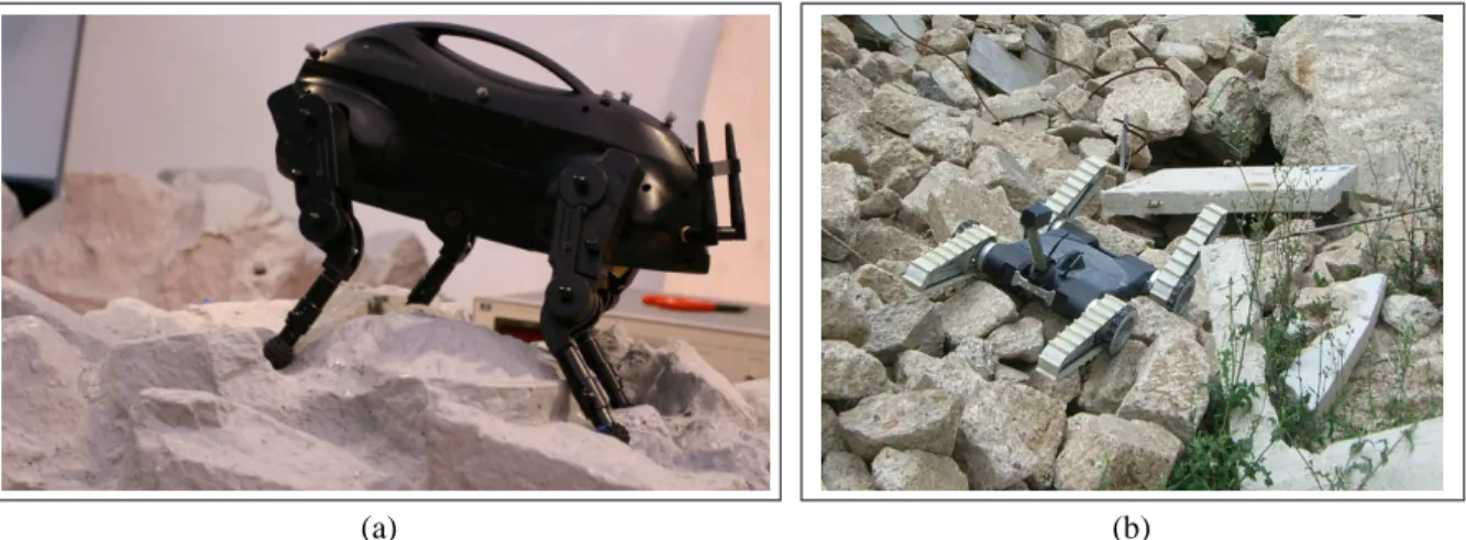
While the utility of robots performing such sensing tasks may be obvious, creating the robots is certainly not. Operating within a partially collapsed building, or other similar environments requires a robot to be able to traverse cluttered, obstacle strewn terrain. Over the years, researchers have tackled these problems and designed a number of ground robot systems, such as the ones shown in figure 1-2 capable of traversing rough terrain. Despite the progress toward this goal, it is still an active area of research and no matter how far the field advances, there will always be some terrain which a ground robot is simply not physically capable of climbing over. Many researchers have therefore proposed the use of Micro Air Vehicles (MAVs) as an alternative robotic platform for rescue tasks and a host of other applications.

(a) (b)

Figure 1-2: Two ground robots designed for traversing rough terrain. [Photo credit: (a)DARPA Learning Locomotion Project at MIT, (b) NIST]

Indeed, MAVs are already being used in several military and civilian domains, includ-ing surveillance operations, weather observation, disaster relief coordination, and civil en-gineering inspections. Enabled by the combination of GPS and MEMs inertial sensors, researchers have been able to develop MAVs that display an impressive array of capabili-ties in outdoor environments without human intervention.

Unfortunately, most indoor environments and many parts of the urban canyon remain without access to external positioning systems such as GPS. Autonomous MAVs today are thus very limited in their ability to operate in these areas. Traditionally, unmanned vehi-cles operating in GPS-denied environments can rely on dead reckoning for localization, but

these measurements drift over time. Alternatively, with onboard environmental sensors, si-multaneous localization and mapping (SLAM) algorithms build a map of the environment around the vehicle from sensor data while simultaneously using the data to estimate the vehicle’s position. Although there have been significant advances in developing accurate, drift-free SLAM algorithms in large-scale environments, these algorithms have focused al-most exclusively on ground or underwater vehicles. In contrast, attempts to achieve the same results with MAVs have not been as successful due to a combination of limited pay-loads for sensing and computation, coupled with the fast and unstable dynamics of air vehicles. While MAV platforms present the promise of allowing researchers to simply fly over rough and challenging terrain, MAVs have their own host of challenges which must be tackled before this promise can be realized.

1.1

Key Challenges

In the ground robotics domain, combining wheel odometry with sensors such as laser range-finders, sonars, or cameras in a probabilistic SLAM framework has proven very suc-cessful [92]. Many algorithms exist that accurately localize ground robots in large-scale environments; however, experiments with these algorithms are usually performed with sta-ble, slow moving robots such as the ones shown in figure 1-3, which cannot handle even moderately rough terrain.

Unfortunately, mounting equivalent sensors onto a MAV and using an existing SLAM algorithms does not result in the same success. MAVs face a number of unique challenges that make developing algorithms for them far more difficult than their indoor ground robot counterparts. The requirements and assumptions that can be made with flying robots are sufficiently different that they must be explicitly reasoned about and managed differently.

Limited Sensing Payload MAVs have a maximum amount of vertical thrust that they can generate to remain airborne, which severely limits the amount of payload available for sensing and computation compared to similar sized ground vehicles. This weight limita-tion eliminates popular sensors such as SICK laser scanners, large-aperture cameras and

Figure 1-3: Examples of robots commonly used for SLAM research. [Photo credit: Cyrill Stachniss]

high-fidelity IMUs. Instead, indoor air robots must rely on lightweight Hokuyo laser scan-ners, micro cameras and lower-quality MEMS-based IMUs, which generally have limited ranges, fields-of-view and are noisier compared to their ground equivalents.

Limited Onboard Computation Despite the advances within the community, SLAM al-gorithms continue to be computationally demanding even for powerful desktop computers and are therefore not usable on today’s small embedded computer systems that might be mounted onboard MAVs. The computation can be offloaded to a powerful ground-station by transmitting the sensor data wirelessly; however, communication bandwidth then be-comes a bottleneck that constrains sensor options. For example, camera data must be com-pressed with lossy algorithms before it can be transmitted over wireless links, which adds noise and delay to the measurements. The delay is in addition to the time taken to transmit the data over the wireless link. The noise from the lossy compression artifacts can be par-ticularly damaging for feature detectors that look for high frequency information such as corners in an image. Additionally, while the delay can often be ignored for slow moving, passively stable ground robots, MAVs have fast and unstable dynamics, making control under large sensor delay conditions impossible.

Figure 1-4: Ground truth velocities (blue) compared with integrated acceleration (green). In just 10 seconds, the velocity estimate diverged by over .25m/s. Position estimates

would diverge commensurately faster.

Indirect Relative Position Estimates Air vehicles do not maintain physical contact with their surroundings and are therefore unable to measure odometry directly, which most SLAM algorithms require to initialize the estimates of the vehicle’s motion between time steps. Although one can compute the relative motion by double-integrating accelerations, lightweight MEMs IMUs are often subject to unsteady biases that result in large drift rates, as shown in figure 1-4. We must therefore recover the vehicle’s relative motion indirectly using exteroceptive sensors, and computing the vehicle’s motion relative to reference points in the environment.

Fast Dynamics MAVs have fast dynamics, which results in a host of sensing, estima-tion, control and planning implications for the vehicle. When confronted with noisy sensor measurements, filtering techniques such as Kalman Filters are often used to obtain better estimates of the true vehicle state. However, the averaging process implicit in the these filters mean that multiple measurements must be observed before the estimate of the un-derlying state will change. Smoothing the data generates a cleaner signal, but adds delay to the state estimates. While delays may have insignificant effects on vehicles with slow

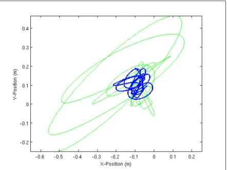
dy-namics, the effects are amplified by the MAV’s fast dynamics. This problem is illustrated in figure 1-5, where we compare the normal hover accuracy to when state estimates are delayed by150ms. While our vehicle is normally able to hover with an RMS error of 6cm,

with the delay, the error increases to18cm.

Figure 1-5: Comparison of the hover accuracy using the state estimates from our system without additional delay (blue), and the accuracy with150ms of delay artificially imposed

(green).

Need to Estimate Velocity In addition, as will be discussed further in Section 3.3, MAVs such as the quadrotor that we use are well-modeled as a simple2nd_{-order dynamic system}

with no damping. The underdamped nature of the dynamics model implies that simple pro-portional control techniques are insufficient to stabilize the vehicle, since any delay in the system will result in unstable oscillations, an effect that we have observed experimentally. We must therefore add damping to the system through the feedback controller, which em-phasizes the importance of obtaining accurate and timely state estimates for both position and velocity. Traditionally, most SLAM algorithms for ground robots completely ignore the velocity states.

Constant Motion Unlike ground vehicles, a MAV cannot simply stop and perform more sensing when when its state estimates have large uncertainties. Instead, the vehicle is likely

to be unable to estimate its velocity accurately, and as a result, it may pick up speed or oscillate, degrading the sensor measurements further. Therefore, planning algorithms for air vehicles must not only be biased towards paths with smooth motions, but must also explicitly reason about uncertainty in path planning, as demonstrated in [41]; motivating our exploration strategy in section 3.5.

3D Motion Finally, MAVs operate in a truly 3D environment since they can hover at

different heights. While it is reasonable for a ground robot to focus on estimating a2D map

of the environment, for air vehicles, the2D cross section of a 3D environment can change

drastically with height and attitude, as obstacles suddenly appear or disappear. However, if we explicitly reason about the effects of changes due to the3D structure of the environment,

we have found that a2D representation of the environment is surprisingly useful for MAV

flight.

1.2

Problem Statement

In the research presented in this thesis, we sought to tackle the the problems described above and develop a system that integrates sensing, planning, and control to enable a MAV to autonomously explore indoor environments. We seek to do this using only onboard sensing and without prior knowledge of the environment.

1.3

Related Work

In recent years, the development of autonomous flying robots has been an area of increasing research interest. This research has produced a number of systems with a wide range of capabilities when operating in outdoor environments. For example vehicles have been developed that can perform high-speed flight through cluttered environments [84], or even acrobatics [20]. Other researchers have developed systems capable of autonomous landing, terrain mapping [90], and a host of high level capabilities such as coordinated tracking and planning of ground vehicles [12], and multi-vehicle coordination [32, 93, 17]. While these

are all challenging research areas in their own right, and pieces of the work (such as the modeling and control techniques) carry over to the development of vehicles operating in indoors, these systems rely on external systems such as GPS, or external cameras [63] for localization. In our work, we focus on flying robots that are able to operate autonomously while carrying all sensors used for localization, control and navigation onboard. This is in contrast to approaches taken by other researchers [45, 43] who have flown indoors using position information from motion capture systems, or external cameras [8, 9].

Outdoor Visual Control While outdoor vehicles can usually rely on GPS, there are many situation where it would be unsafe for a vehicle to rely on it, since signal can be lost due to multipath fading, satellites being occluded by buildings and foliage, or even intentional jamming. In response to these concerns, a number of researchers have developed systems that rely on vision for control of the vehicle. The capabilities of these systems include visual servoing relative to a designated target [64], landing on a moving target [80], and even navigation through urban canyons [47]. While the systems developed by these researchers share many of the challenges faced by indoor MAVs, they operate on vehicles that are orders of magnitude larger, such as the one shown in figure 1-6, with much greater sensing and computation payloads.

Figure 1-6: The USC AVATAR helicopter, built around a Bergen Industrial Twin RC helicopter, which is a common helicopter platform for outdoor experiments. [Photo credit: Dr. Stefan Hrabar and the USC Robotic Embedded Systems Laboratory (http://robotics.usc.edu/resl)]

Indoor Obstacle Avoidance Using platforms that are of a similar scale to the ones tar-geted in this thesis, several researchers [75, 14, 62] use a small number of ultrasound or infrared sensors to perform altitude control and basic obstacle avoidance in indoor environ-ments. While their MAVs are able to hover autonomously, they do not achieve any sort of goal directed flight that would enable the systems to be controlled at a high level such that they could be used for higher level applications.

Known Structure Instead of using low resolution sonar and infrared sensors, several au-thors have attempted to fly MAVs autonomously indoors using monocular camera sensors. To enable the vision processing to be tractable, they make very strong (and brittle) assump-tions about the environment. For example, Tournier et al. [95] performed visual servoing over known Moire patterns to extract the full 6 dof state of the vehicle for control; and Kemp [54] fit lines in the camera images to the edges of a3D model of an office

environ-ment with known structure. Reducing the prior knowledge slightly, Johnson [49] detects lines in a hallway, and used the assumption of a straight hallway to back out the vehicle pose. Similarly, Celik et al presented their MVCSLAM system in [19], which tracks cor-ner features along the floor of a hallway. While impressive, it is unclear how their work could be extended to other environments. Their applicability is therefore constrained to environments with specific features, and thus may not work as well for general navigation in GPS-denied environments.

Using a2D laser scanner instead of a camera, prior work done in our group [41]

pre-sented a planning algorithm for a quadrotor helicopter that is able to navigate autonomously within an indoor environment for which there is a known map. Recently, [10, 35] designed quadrotor configurations that were similar to the one presented in [41]. Grzonka et al. and Angeletti et al. [10] scan-matched successive laser scans to hover their quadrotor heli-copter, while [35, 36] used particle filter methods to globally localize their MAV. However, none of these papers presented experimental results demonstrating the ability to stabilize all 6 degrees of freedom of the MAV using the onboard sensors, and all made use of prior maps, an assumption that is relaxed in this thesis.

Indoor SLAM Finally, perhaps the closest work to ours was that of Ahrens [7], where monocular vision SLAM was used to stabilize a quadrotor. Extracted corner features were fed into an extended Kalman filter based vision-SLAM framework, building a low-resolution3D map sufficient for localization and planning. Unfortunately, an external

mo-tion capture system was used to simulate inertial sensor readings, instead of using an on-board IMU. As such, their system was constrained to the motion capture volume where they had access to the high quality simulated IMU. It remains to be seen whether the work can be extended to use lower quality acceleration estimates from a more realistic MAV-scale IMU.

Adopting a slightly different approach, Steder et al [86] mounted a downward-pointing camera on a blimp to create visual maps of the environment floor. While interesting al-gorithmically, this work does not tackle any of the challenges due to the fast dynamics described in section 1.1.

Where many of the above approaches for indoor flight fall short is that they did not consider the requirements for stabilizing the MAV both locally and in larger scale envi-ronments in a coherent system. The previous work either focused on local hovering and obstacle avoidance in known, constrained environments, or attempted to tackle the full SLAM problem directly, without stabilizing the vehicle using local state estimation meth-ods. SLAM processes are generally too slow to close the loop and control an unsteady MAV, resulting in systems that work well in simulation, however are unworkable when applied on real hardware. In our work, we developed a multi-layer sensing and control hierarchy which tackles both of these challenges in a coherent system.

1.4

Contributions

In this thesis, I present the design, implementation, and validation of a system for localizing and controlling the quadrotor helicopter shown flying in figure 1-7, such that it is capable of autonomous goal directed flight in unstructured indoor environments. As such, the primary contribution is the development of the working system. While the system builds upon existing work from the robotics community, many of the individual components required

Figure 1-7: A photo of our vehicle flying autonomously in an unstructured indoor environ-ment

adaptation to be used on MAVs. More specifically, the contributions of this thesis are:

1. Development of a fully autonomous quadrotor that relies only on onboard sensors for stable control, without requiring prior information (maps) about the environment.

2. A high-speed laser scan-matching algorithm that allows successive laser scans to be compared in real-time to provide accurate velocity and relative position information.

3. An Extended Kalman Filter data fusion module, and algorithm for tuning it that provides accurate real-time estimates of the MAV position and velocity

4. A modified SLAM algorithm that handles the3D environment structure in a 2D map

5. A framework for performing dense reconstruction and mapping of the full3D

envi-ronment around the vehicle

6. A visual object tracking system that allows the vehicle to follow a target designated in a camera image.

Figure 1-8: Schematic of our hierarchical sensing, control and planning system. At the base level, the onboard IMU and controller (green) creates a tight feedback loop to stabilize the MAV’s pitch and roll. The yellow modules make up the real-time sensing and control loop that stabilizes the MAV’s pose at the local level and avoids obstacles. Finally, the red modules provide the high-level mapping and planning functionalities.

1.5

System Overview

To compute the high-precision, low delay state estimates required for indoor flight, we designed the 3-level sensing and control hierarchy, shown in figure 1-8, distinguishing processes based on the real-time requirements of their respective outputs. The first two layers run in real-time, and are responsible for stabilizing the vehicle and performing low level obstacle avoidance. The third layer is responsible for creating a consistent global map of the world, as well as planning and executing high level actions.

At the base level, the onboard IMU and processor creates a very tight feedback loop to stabilize the MAV’s pitch and roll, operating at1000Hz. At the next level, fast,

high-resolution relative position estimation algorithms, described in chapter 2, estimate the ve-hicle’s motion, while an Extended Kalman Filter (EKF) fuses the estimates with the IMU outputs to provide accurate, high frequency state estimates. These estimates enable the LQR-based feedback controller to hover the MAV stably in small, local environments. In

addition, a simple obstacle avoidance module ensures that the MAV maintains a minimum distance from observed obstacles.

At the top layer, a SLAM algorithm uses the EKF state estimates and incoming laser scans to create a global map, ensuring globally consistent state estimates by performing loop closures. Since the SLAM algorithm takes 1-2 seconds to incorporate incoming scans, it is not part of the real-time feedback control loops at the lower levels. Instead, it provides delayed correction signals to the EKF, ensuring that our real-time state estimates remain globally consistent. Finally, a planning and exploration module enables the vehicle to plan paths within the map generated by the SLAM module, and guide the vehicle towards unexplored regions.

1.6

Outline

In the chapters 2 and 3, I describe the components of the system that enable flight in un-constrained indoor environments. Chapter 2 covers the algorithms for obtaining relative position estimates using either high-speed laser scan-matching or stereo visual odometry. Chapter 3 describes how these estimates are used in the complete system, along with the details of the system components.

After describing the complete system, I describe the hardware we use, and present experimental results validating our design and demonstrating the capabilities of our system in chapter 4.

In chapter 5 I present a framework for performing dense mapping of the 3D

environ-ment around the vehicle, which would enable generating motion plans in3D. Finally, in

chapter 6 I present a vision based object tracking system that allows the vehicle to perform high level tasks such as following a person before presenting future work and concluding remarks in chapter 7.

Chapter 2

Relative Position Estimation

In this chapter I describe the algorithms used for estimating the MAV’s relative position in real-time. Both laser and stereo-vision based solutions are presented and compared. The high quality relative position estimates provided by these algorithms are the key enabling technology for indoor flight.

The stereo-vision based visual odometry solution was developed in collaboration with Markus Achtelik [6].

2.1

Introduction

MAVs have no direct way to measure their motion, and must therefore rely on sophisticated algorithms to extract synthetic proxies for the wheel encoder based odometry available on ground robots from other sensors. While one may be tempted to double-integrate accel-eration measurements from inertial sensors to obtain relative position estimates, the drift rates of small lightweight MEMs IMUs are prohibitively high. Instead one must rely on exteroceptive sensors, matching incoming measurements with one another to back out the vehicle’s relative motion. This process can be performed on both laser scans and camera images, each having distinct advantages and disadvantages in terms of their computational requirements, accuracy, and failure modes.

While air vehicles do not have the luxury of using wheel odometry to measure relative position, many ground robots have faced similar challenges, since in many situations the

estimates from wheel odometry can be quite poor, such as when a robot is traversing rough terrain. As a result, there has been considerable work on developing relative position esti-mation algorithms for ground robots. Researchers have often found that the performance of both scan-matching and visual odometry greatly outperforms wheel odometry [70, 46]. Al-though the algorithms have largely been developed for ground robots, they can be adapted for use on MAVs, but with the additional challenging requirements of both high resolution matching and fast real-time performance. The high resolution matching is particularly im-portant due to the need to estimate the velocity of the MAV for control purposes. To obtain these velocity estimates, we must differentiate the computed relative position estimates. So while a positional error of a few centimeters may be insignificant for a ground robot, when divided by the time between scans, a few centimeter error in position will result in a large error in velocity. In addition, since MAVs operate in the full 3D environment, we must ensure that the algorithms are robust to motion in all 6 degrees of freedom.

The relative position estimation algorithms can generally be broken down into two sub-routines:

1. Correspondence: Find matches between “features” in the measurements

2. Motion Extraction: Given sets of corresponding features, determine the optimal rigid body transform between them.

As we shall see, the existing algorithms take different approaches to each of these subrou-tines, with different robustness, accuracy, and computational complexity properties.

In addition, different types of sensors have unique characteristics that lead to varying levels of effectiveness in different environments. Laser range-finders operate by emitting a beam of laser light, and measuring the time until the beam is reflected back onto a photo sensor. This process provides a measurement of the distance to the nearest obstacle in the direction of the laser beam. By sweeping the laser beam in a circle, and taking suc-cessive point measurements at fixed intervals, the sensor is able to generate a “scan” of the environment that contains the range to the nearest obstacle at a fixed set of bearings. When converted from this polar-coordinate form to Cartesian coordinates we obtain a set of points such as the ones shown in Figure 2-1(a). Since laser range finders provide a set

of distances, laser scans can only be matched when the environment has unique physical structure or shape. As a result, the matching process can fail around homogeneous building structures such as long corridors. In addition, since the sensors only generate2D slices of

the environments, they cannot make use of structure outside the sensing plane.

In contrast, camera sensors, which measure the intensity of light falling onto a 2D

sensor plane, can make use of information from the full3D environment around the vehicle.

However, camera sensors only measure the intensity of the light, and therefore do not provide direct information about the underlying3D structure that generated the image. To

be able to extract that information from image data the environment must contain unique visual features, and requires sophisticated image processing. In general, camera sensors have more limited angular field-of-views and are computationally intensive to work with.

Different exteroceptive sensors are therefore better suited for autonomous MAV op-eration under different environmental conditions. However, since the laser scanner and cameras rely on different environmental features, they should have complementary fail-ure modes. As a result, integrating both sensors onto a single MAV platform will enable autonomous navigation in a wide range of generic, unstructured indoor environments.

2.2

Laser Scan-Matching

Laser scan-matching algorithms must solve the following problem: given two overlapping laser range scans St ∈ ℜ2×n and St−1 ∈ ℜ2×n, find the optimal rigid body transform

∆ ∈ SO(3) = [R, t] that aligns the current laser scan with the previous scan such that

applying the transform∆ to St−1, denoted∆ ⊗ St−1, results in a scan that is close toSt.

To find the best alignment, one needs a method for scoring candidate transforms based on how well they align to past scans. The first challenge in doing this is that laser scanners provide individual point measurements of locations in the environment. Successive scans will generally not measure the same points in the environment due to the motion of the vehicle. Each scan-matching algorithm must therefore find a way to overcome this issue to find correspondences. This is usually done in one of3 ways:

1. Point-to-Point: The individual points from the current scan are matched directly to one (or multiple) points in the previous scan, such as in the Iterative Closest Point (ICP) [101] algorithm described below.

2. Feature-to-Feature: Points are grouped into higher level features such as corners and lines that are then matched, such as in the HAYAI algorithm [58]. Since the features can often be accurately corresponded directly, the resulting motion estimate can be computed in closed form, without needing the iterative refinement of the cor-respondences used in ICP.

3. No-Correspondences: The points from previous scans are used to create a likelihood map, and the current scan is matched to this map by searching for the pose which gives the scan a maximum likelihood with respect to the map. This is the approach taken by, Vasco [39, 2], Olson [70], and our scan-matcher. One of the benefits of this approach is that it does not require explicit correspondences to be computed.

When considering the algorithm to use on a MAV, robustness to outliers is particularly important. The laser scanner measures ranges in a 2D plane, while the vehicle moves in the full 3D environment. Motion out of the plane of the laser can result in portions of the laser scan changing dramatically. As a result, while the scan-matching algorithms for ground robots must only worry about errors due to sensor noise, which is generally fairly low, our algorithm must be very robust to regions of the scan changing due to 3D effects. This requirement essentially precludes the use of the feature based approaches since they are very susceptible to incorrect correspondences between features.

2.2.1

Iterative Closest Point

The iterative closest point algorithm [101] is one of the simplest and most commonly used algorithms for laser scan-matching. It is an iterative algorithm which alternates between finding correspondences between individual points and their nearest neighbor, and finding the optimal rigid body transform that minimizes the Euclidean distance between the points, as shown in algorithm 1. The optimal rigid body transform (in a least-squares sense) be-tween two sets of corresponded points can be computed in closed form [97], which is

(a) (b) (c)

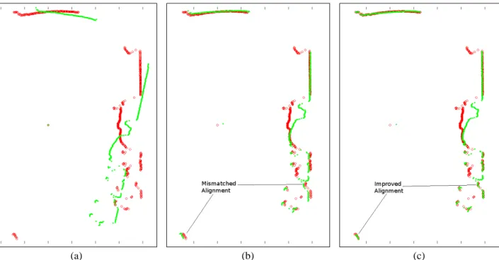
Figure 2-1: (a) The original set of points for 2 laser scans, showing a region with significant differences due to 3D effects. (b)The alignment computed by ICP. Notice the misalignment due to poor correspondences in the non-matching region. (c) The alignment computed by our algorithm, which robustly matches the two scans.

attractive due to its computational efficiency. While the rigid body transform for a given set of corresponding points is computed in closed form, the algorithm as a whole does not necessarily find the global optimum, since it may be susceptible to local minima when computing the point correspondences.

While this basic form of the ICP algorithm is extremely simple and fairly efficient, it suffers from robustness issues in the presence of regions of the scans that do not match, such as the scans in figure 2-1(a). The region in the bottom right of the figure has considerable differences between the two scans due to out of plane motion. Since the ICP algorithm finds correspondences for these points despite the fact that they have no match, it skews the computed transform, resulting in the slight rotation between the scans in figure 2-1(b). Many researchers have proposed variants of this basic ICP algorithm, which use a different distance function, or add an outlier rejection step which improves the matching robustness and/or efficiency [78, 77, 66]. However these variants add significant complexity without solving the fundamental problem: corresponding points which are not measurements of the

Algorithm 1 The Iterative Closest Point algorithm Require: S1 andS2 (the scans to be matched)

Require: ∆ (initial guess of the transformation)

while∆ not converged do ˆ

S2 = ∆ ⊗ S2 (projectS2 using current transform)

for x1_i ∈ S1 do y_i = argmin x2 i∈ ˆS2 ||x1 i − x2i||2 end for ∆ = [R, t] = argmin [R,t] N X i=1 ||Ryi+ t − x1i||2 end while

same point in the environment.

2.2.2

Map Based Probabilistic Scan-Matching

As an alternative to computing the correspondences explicitly, a challenging and error prone process, one can create an occupancy grid map M from previous scans [91], and

then match the new scan against that map. Each cell in the map stores the likelihood of the

ith laser return being measured at the point xias

P (xi|M) (2.1)

This map then allows us to compute the likelihood for an entire scan by computing the likelihood that all laser readings fall where they do. Assuming that each of the point measurements in a laser scan are independent, the likelihood for an entire scan can be computed as P (S|M) = N Y i=1 P (xi|M) (2.2)

By searching over candidate rigid body transforms∆ ∈ SO(3) to find the one that

maxi-mizes the likelihood of the laser reading, we can then find the optimal∆∗ _{which provides}

the best alignment of the incoming laser scan:

∆∗ = argmax

∆

where∆ ⊗ S is the set of laser points S transformed by the rigid body transform ∆

This is the approach used by the Vasco scan-matcher in the Carmen robotics toolkit [39, 2], and the scan-matcher developed by Olson [70, 69], upon which our work is based. While similar in concept, the algorithms differ in their methods for constructing and search-ing the likelihood map.

In Vasco the map is constructed by storing the number of times each cell is hit by a laser measurement and then integrating over small errors with Gaussian smoothing. This smoothing captures the uncertainty present in the laser measurements. There is noise in both the range and bearing of each laser measurement, which means that points near a cell that is hit should also have an increased likelihood of generating a laser return. The optimal scan alignment with respect to the map is then computed by performing a greedy hill-climbing process. Starting from an initial guess of the correct transform, Vasco successively tests new transforms around the current best, and keeps modifications that increase the likelihood of the resulting transformed scan as shown in algorithm 2.

Algorithm 2 Vasco Hill Climbing Algorithm Require: S (scan to be matched)

Require: M (the likelihood map)

Require: ∆ (initial guess of the transformation)

L ← P (∆ ⊗ S|M) (evaluate likelihood of initial guess)

while∆ not converged do

for ˆ∆ = ∆ + δ ∈ {F orward, Back, Lef t, Right, T urnLef t, T urnRight} do

if P ( ˆ∆ ⊗ S|M) > L then L ← P ( ˆ∆ ⊗ S|M) ∆ ← ˆ∆ end if end for end while

While this scan-matching method has proven quite successful, and is an improvement over ICP, it still has two flaws which are corrected in Olson’s approach. First, since laser scanners have a limited angular resolution, readings far from the sensor will be spaced far apart. As a result, if a subsequent measurement at timet + 1 falls in between two readings

taken at time t, the later measurement will appear to be low likelihood despite the fact

Figure 2-2: A cross section of the pose likelihood map showing the likelihood of a scan at different translations, with a fixed rotation. Notice the multiple local maxima.

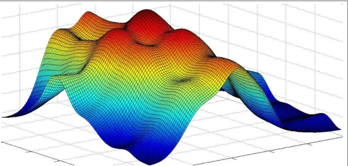
MAVs is the use of the hill-climbing strategy. As can be seen in figure 2-2, which shows a 2D cross section of the 3D pose likelihood map, there are several local maxima. Unless we were lucky enough to start near the global optima, hill climbing is unlikely to find it. Vasco mitigates this problem by using the estimate from wheel odometry to initialize the hill-climbing process, however MAVs do not have that luxury.

2.2.3

Robust High-Speed Probabilistic Scan-Matching

After surveying the algorithms available for performing laser scan-matching we decided to base our algorithm on the one developed by Olson, which focused on robustness, while still managing to be computationally efficient through careful implementation. Like Vasco, Olson’s method performs probabilistic scan matching using a map, however it differs in two significant ways:

1. The points in a laser scan are connected into a set of piece-wise linear contours, creating continuous surfaces in the map instead of individual points.

align-ments instead of using hill climbing.

Our algorithm uses this same approach, however we made several changes to adapt it such that it could handle the 3D environment and run in real-time with the high resolution

re-quired by the MAV. In addition, we added a “polishing” step after the exhastive search where we use the gradient ascent method shown in algorithm 2 to refine the pose estimate. Since we start the gradient ascent from the optimum found by exhaustive search, the opti-mization is very fast, and we are more likely to find the global optima than if we did not perform the exhaustive search first.

Local Map Generation

To find the best alignment for an incoming laser scan, one needs a method for scoring candidate poses based on how well they align to past scans. As mentioned above, laser scanners provide individual point measurements. Successive scans will generally not mea-sure the same points in the environment since when the laser scanner moves the meamea-sured points are shifted accordingly. Since the points do not necessarily measure the same points, attempting to correspond points explicitly can produce poor results due to incorrect match-ing. However, many indoor environments are made up of planar surfaces with a2D cross

section that is a set of piecewise linear line segments. While individual laser measurements do not usually measure the same point in the environment, they will usually measure points on the same surface. We therefore model the the environment as a set of polyline contours. Contours are extracted from the laser readings by an algorithm that iteratively connects the endpoints of candidate contours until no more endpoints satisfy the joining constraints as shown in algorithm 3.

The algorithm prioritizes joining nearby contours, which allows it to handle partially transparent surfaces such as the railings in the environment depicted by Figure 2-3(a). If we instead tried to simply connect adjacent range readings in the laser scan, there would be many additional line segments connecting points on either side of the corner. Candidate contour merges are scored and stored in a Min-heap data-structure, which allows the best candidate to be extracted efficiently. As a result, the overall contour extraction algorithm takes around0.5ms to process a 350 point scan on modern hardware.

Algorithm 3 Extract Contours Require: S (set of points)

Require: priority queue for candidate joins {parent,child,score} sorted by score priority queue ← ∅

for x∈ S do

addjoin of x with nearest free point to priority queue

end for

whilepriority queue 6= ∅ do

remove bestjoin from priority queue

ifjoin.parent already has a child then

discardjoin

else if connectingjoin.child to join.parent incurs too much cost then

discardjoin

else ifjoin.child already has a parent then

addjoin of x with nearest free point to priority queue

else

merge the contours ofjoin.child and join.parent

end if end while

return Final set of contours

Once we have the set of contours extracted from the previous scan, we can evaluate the likelihood of an alignment of the current scan. We assume that all point measurements in a scan are independent, and we compute the likelihood of alignment of a scan as the product of likelihoods for each individual point in the scan. As mentioned above, laser range-finders provide noisy measurements of the range and bearing of obstacles in the environment. While each of these degrees of freedom has an independent noise term, we assume a radially symmetric sensor model for simplicity. Our noise model approximates the probability of a single lidar point(x, y) as proportional to the distance d to the nearest

contourC, such that

P (x, y|C) ∝ e(−d/σ)_{, (2.4)}

where σ is a variance parameter that accounts for the sensors noise characteristics. As

was done for Vasco, we compute a grid-map representation where each cell represents the approximate log-likelihood of a laser reading being returned from a given location.

For most ground robotics applications, a map resolution of10cm or more is often

(a) (b)

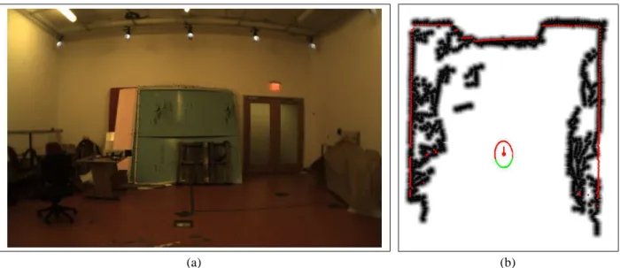
Figure 2-3: (a) Contours (blue lines) extracted from the raw laser measurements alongside the raw laser readings (red dots). Notice how the contour extraction algorithm handles the partially transparent railing on the left. (b) The resulting likelihood map generated from the contours. Brighter colors (red) indicates higher likelihood.

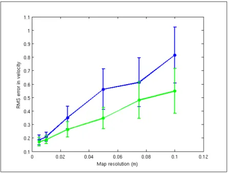
errors in the position are magnified significantly, we require a high resolution map with a cell size less than1cm. For example, if we use a map resolution of 10cm and the laser scans

arrive at40Hz, an alignment that is rounded off by half a cell would result in an error on

the order of2m/s. Since the vehicle is usually moving at less than 1m/s this error would

be very significant. This effect is seen in the experimental results shown in Figure 2-5. While generating these high resolution maps is computationally intensive, one can leverage their sparsity to make generating them tractable. If one examines a likelihood map such as the one shown in figure 2-3(b), one quickly realizes that with any reasonable value ofσ, the vast majority of cells will be zero. So, while conventional methods compute

a value for every cell in the map, and therefore require at leastO(n2_{) operations, where n}

is the number of cells along an edge, we developed a likelihood map generation algorithm that exploits the sparsity in the grid map, resulting in a computational complexity ofO(m)

wherem ≪ n2 _{is the number of occupied cells.}

In Olson’s work, he computed the likelihood map by restricting the likelihood calcula-tion to a local window around each line segment in the contour, and computing the distance

from each pixel in the window to the line segment. While an improvement over computing the distance to the nearest line segment for the entire map, this method still does not run in real-time at the required resolution. Computing the distance to the line segment for each pixel is computationally intensive, and to make matters worse, the windows around each line segment have significant overlap, which means that each pixel ends up being modified many times.

In order to create the high resolution likelihood maps in real-time, we developed a drawing primitive that explicitly “draws” the non-zero likelihoods around each line seg-ment. This primitive does not require us to compute the distance to the line segment for each pixel and has much less overlap in the pixels around the line segment endpoints that are touched such that in general each pixel is only written once. We accomplish this by sliding a Gaussian shaped kernel along the pixels of the line segment (as output by the Bre-senham line drawing algorithm [16]), applying a max operator between the current map

value and the kernel’s value. Naively using a square kernel, with values set based on equa-tion 2.4 would result in cells being written many times as the kernel slides along the line; however, one can avoid this problem by using a 1 pixel wide horizontal or vertical cross section of the kernel depending on the slope of the line. For lines that are not perfectly horizontal or vertical, this kernel must be stretched by1/cos(s), where s is the slope of the

line. As a final optimization, the kernelmax operation can be performed using optimized

matrix libraries. With the new drawing primitive, creating the likelihood map simply re-duces to drawing all the line segments in the extracted contours, which takes around20ms

even for extremely large7.5mm resolution likelihood maps.

We create the map from a set of k previous scans so that the relative position and

ve-locity estimates are consistent within the local map. Comparing a new scan to an aggregate of previous scans gives much more accurate position estimates than comparing each scan only to the scan from the previous time step, as it reduces the integration of small errors over time. For example if the vehicle is stationary, the very first scan received should be the only scan in the map so that the position estimate will remain drift free. On the other hand, if we only compare each pair of incoming scans, any small errors on previous position esti-mates will be retained and integrated into the current position estimate, resulting in drift. In

addition, since the likelihood map must be recreated every time a scan is added or removed from the map, comparing each pair of incoming scans is computationally inefficient.

In both Vasco, and Olson’s work a new scan is added to the map only after the vehi-cle has moved some minimum distance. This heuristic is meant to ensure that scans are added to the map with enough overlap to match them effectively, while not adding scans unnecessarily frequently. The heuristic works well for ground vehicles where in general the scans only change due to motion of the vehicle. However, on a MAV the heuristic is problematic due to the drastic changes to the scan that can occur as the vehicle changes height. When the vehicle changes height, the environment may change, such that large portions of the map are quite different, despite the fact that the vehicle has not moved very far in any dimension. In this situation, we want to add the new scan to the map so that we can match against this region as well. However, if the environment has vertical walls such that the cross-section does not change as the vehicle changes height, then we do not want to add the new scan. As a result, we use a new policy whereby scans are added when they have insufficient overlap with the current map. To do this, we compute the fraction of points in an incoming scan that are above a given likelihood in the current map. When this fraction drops below a threshold, the new scan is added to the map. The threshold is set high enough that incoming scans are still able to be matched accurately, but low enough that scans are not added too often. The new heuristic reduced the amount of drift incurred by in the scan-matching process compared to the distance based one.

In addition to mitigating drift, constructing the map from multiple recent scans handles 3D effects nicely. As can be seen in figure 2-4(b), areas that vary considerably with height, such as the sides of the room, get filled in such that the entire area has high likelihood. The likelihood of a laser point being measured in those areas become almost uniform, while the likelihoods in areas that remain constant, such as the corners of the room in figure 2-4(b), are strongly peaked. Since the entire area has high likelihood its influence on the matching process will be reduced.

(a) (b)

Figure 2-4: (a) A cluttered lab space (b) The resulting likelihood map generated by the scan-matcher after changing heights, with the current scan overlaid. The sides of the room are very cluttered, resulting in an almost uniform distribution in some areas, while the corner remains sharply peaked and provides good alignment.

Scan-to-Map Alignment

Once we have computed the likelihood map, the second task is to find the best rigid body transform ∆∗ _{for each incoming scan with respect to the current likelihood map. Many}

scan-matching algorithms such as Vasco use gradient descent techniques to optimize the values of the transform. However, as we mentioned in section 2.2.2, the three dimensional pose likelihood space is often very complicated, even for fairly simple environments. As a result, we chose to follow Olson, and use a very robust, if potentially computationally inef-ficient, exhaustive search over a three-dimensional volume of possible poses. The number of candidate poses in the search volume is determined by the size of the search volume (how far we search) and the translational and angular step size (how finely we search). Un-fortunately, the chosen step sizes limit the resolution with which we can match the scans, so we modify Olson’s approach to perform gradient ascent from the global optima chosen by the exhaustive search.

While this exhaustive search might initially seem hopelessly inefficient, if implemented carefully, it can be done very quickly. A naive implementation of this search might perform the search using three nested for-loops to iterate through all poses in the search volume. A

fourth for-loop would then iterate over all points in the scan, projecting them, and looking up their likelihood in the map. Much of the computational cost in this search is taken up by performing the projection of the laser scan in the innermost loop. However, for a given candidate angle θ, the projected points in a laser scan are related by a simple translation.

As a result, if we iterate overθ in the outermost loop, and perform the rotation component

of the projection of each point there, the inner loops only have to perform a simple addition to complete the projection. Furthermore, if we set the resolution of the likelihood map to be equal to the translational step size, then the set of likelihoods for all translations of a test point are contained in the cells that surround the test point in the map. Iterating over the translational search window is therefore much faster since the innermost loop which iterates over the points only performs a table lookup and does not have to project the test points. As a final optimization, the entire translational search window can be accumulated into the3D pose likelihood map in one step using the optimized image addition functions

available in the Intel Performance Primitives [23], which provide a factor of2 speed up.

The optimized exhaustive search implementation is considerably faster than a naive implementation, however, we still must ensure that the area over which we search is not too large. Since we do not have wheel odometry with which to initialize the scan-matching, we assume that the vehicle moves at a constant velocity between scans. With this starting point, the range of poses that must be searched over can then be selected based on the maximum expected acceleration of the vehicle, which means that at high scan rates, the search volume is manageable.

In Olson’s method, the resolution with which we build the map limits the accuracy with which we can estimate the pose of the vehicle since we match the translational step size to the map resolution. However, step sizes smaller than the map resolution can change the scan likelihood due to points near the boundary between map cells being moved across the boundary. To improve the accuracy of our relative position estimates beyond the resolution used to create the map, we added a polishing step to the scan-to-map alignment where we apply the gradient ascent method described in algorithm 2 to optimize the final pose estimate. Using gradient ascent on top of the exhaustive search retains the robustness of Olson’s method, while improving the accuracy considerably as shown in Figure 2-5. Since

Figure 2-5: Comparison of the RMS error in velocity as a function of the map resolution, and whether gradient ascent polishing was used. The blue line shows the error for each map resolution without performing the gradient ascent polishing step, while the green line shows the same experiment with gradient ascent turned on.

we initialize the gradient ascent from the global optima found by the exhaustive search, the algorithm converges very quickly (usually∼ 1ms), and is likely to find the true global

optima.

In our implementation, we use step sizes (and grid spacing) of 7.5mm in x, y, and .15◦ _{inθ. At this resolution, it takes approximately 5ms to search over the approximately}

15, 000 candidate poses in the search grid to find the best pose for an incoming scan. This

means that we are able to process them at the full40Hz data rate. When a scan needs to be

added to the likelihood map, this is done as a background computational process, allowing pose estimation to continue without impeding the real-time processing path.

Covariance Estimation

In addition to being very robust, computing the best alignment by exhaustive search has the advantage of making it easy to obtain a good estimate of the covariance in the relative-position estimates by examining the shape of the pose likelihood map around the global optimum. This estimate of the covariance is important when we integrate the relative

posi-tion estimates with other sensors in the data fusion module described in secposi-tion 3.2. While the entire pose likelihood map has many local maxima as shown in Figure 2-2, in the im-mediate vicinity of the global optima the pose likelihood is usually a fairly smooth bell shape. If the environment surrounding the vehicle has obstacles in all directions, such as in a corner, the alignment of scans will be highly constrained, resulting in a very peaked pose likelihood map. On the other hand, if the environment does not constrain the alignment, the pose likelihood map will be nearly flat at the top. An example of two such environments is shown in Figure 2.2.3.

(a) (b)

Figure 2-6: Examples of the covariance estimate output by the scan-matcher in different environments. (a) shows an environment with obstacles facing all directions which con-strains the alignment of subsequent scans. (b) shows a hallway environment with very little information along the hallway.

While one could compute the covariance of the goal distribution across all degrees of freedom, for implementation simplicity we compute the covariance in rotation separately from translation, making the assumption that rotation is independent of translation. For translation we look at the2D slice of the pose likelihood map at the optimal rotation. We

then threshold this2D map at the 95th_{percentile, and fit an ellipse to the resulting binary}

image. The area and orientation of this ellipse is used as our estimate of the measurement covariance. For rotation, we find the score of the best translation for each rotation, and look at the width of the resulting bell shaped 1D curve. In the future, we intend to fit a

multi-variate Gaussian directly to the pose likelihood map, following the example of [69].

Contributions

While the scan-matching algorithm described above is based on the original implementa-tion by Olson, it required several modificaimplementa-tions to enable it to be used on the MAV. Specif-ically, these contributions are:

1. The drawing primitive described in section 2.2.3 allows us to generate the high reso-lution likelihood map in real-time.

2. Our notion of a “local map” differs from [70]: scans are added based on insufficient overlap rather than distance traveled.

3. Our use of image addition primitives to accumulate the pose likelihood map.

4. Adapting the search window based on the maximum expected acceleration of the vehicle.

5. Using gradient ascent to refine the relative motion estimate is new. 6. The method for obtaining a covariance estimate is new.

2.2.4

Laser Based Height Estimation

The laser scan-matching algorithms described above only estimate the relative motion of the vehicle inx, y, and θ. In order to control the MAV we must also be able to accurately

estimate the relative position inz. While the laser range-finder normally only emits beams

in a2D plane around the vehicle, we are able to redirect a portion of the beams downward

using a right-angle mirror as shown in Figure 2-7.

Since there are so few range measurements redirected toward the floor, it is impossible to recognize distinctive features that would allow us to match measurements together to disambiguate the motion of the vehicle from changes in the height of the floor. We there-fore cannot use techniques similar to the the scan-matching algorithms described above to simultaneously estimate the height of the vehicle and the floor. If we assume that the

Figure 2-7: Image of the right-angle mirror used to deflect a portion of the laser beams downward to estimate height. The yellow line shows an example beam for visualization.

vehicle is flying over a flat floor, we can use the range measured by the laser scanner,rt,

directly as the estimate of the height of the vehicle at timet. However, if the vehicle flies

over an object such as a table, these height estimates will be incorrect. To make matters worse, flying over the table will appear as a large step discontinuity in the height estimate, as shown in the red line in Figure 2-8(a), which can result in aggressive corrections from the position controller. However, if we look at the vehicle velocity that these height

esti-(a) (b)

Figure 2-8: Plots showing a comparison of the height (a) and velocity (b) estimates from our algorithm (green) alongside the raw measurements (red), and the ground truth (blue). The large discontinuities in the red lines are places where the vehicle flew over the edge of an object. The object was roughly15cm tall.

flies over an object. As a result, we can use the maximum expected acceleration of the vehicle to discard changes in height that are too large, assuming that the height of the floor changed instead of the vehicle. Unfortunately, in reality, both the vehicle and the floor height change simultaneously, so simply discarding the relative height estimate will result in drift over time.

To mitigate this drift, one would ideally adopt a SLAM framework that is able to rec-ognize when the vehicle returns to the same place and closes the loop. However, while this could be done using a camera, or another3D sensor, with only the 2D laser scanner there

is not enough information about the shape of the floor to identify loop closures. We there-fore cannot rely on being able to accurately estimate the height of the floor which would then allow us to estimate our height relative to this floor estimate. Instead, we leverage the assumption that the vehicle would predominantly be flying over open floor, but sometimes fly over furniture or other objects. In this situation, over long time periods the raw height measurements from the downward pointed laser beams are usually correct, but over short time periods they may be perturbed by flying over obstacles. We therefore chose to mitigate the drift in our height estimate by slowly pushing them back towards the raw measurements

rt. While we are still above an object, we do not want to push the height estimate towardrt

since this measurement will not correspond to the actual height of the vehicle. Instead we would like to wait until the vehicle has moved away from the object and is above the floor. Unfortunately, we don’t have a way to identify whether the vehicle is above the floor or a new obstacle. As a result, we make this decision based on thex-y distance the vehicle has

moved since it noticed that the height of the surface underneath it changed. We choose this distance threshold by estimating the average size of objects that the vehicle will encounter. Rather than make a hard decision, we make a soft decision about when corrections should be applied and scale the magnitude of the correction by a logistic function that is centered over the average obstacle size.

More formally, our approach estimates the height of the vehicle, by integrating the difference between successive height range measurementsrtandrt−1filtered such that they

obey the maximum acceleration constraint. This estimate of the height will incur errors when the vehicle goes over obstacles. As a result, we apply a correction term which pushes

the estimate ˆht back towards the raw height,rt, measured by the laser. The magnitude of

this correction is a logistic function of the planar distance d to the last discarded height

measurement.

ˆht= h′+ sgn(rt− h′)

α

(1 + e(σdd−d)¯ ) (2.5)

whereh′ _{is the height estimate after adding the filtered estimate,α is a small scaling}

con-stant on the correction term,σdis a parameter that controls the width of the logistic

func-tion, and ¯d is the center of the logistic function. We chose ¯d to be large enough that we

expect the vehicle to no longer be above an object when the larger corrections are being applied. The current height estimate can be arbitrarily far away from the current measured height, which is why we use only the direction of the error in the correction, and ignore the magnitude. The correction is scaled such that the maximum correction is small enough to induce smooth motions of the vehicle. The complete height estimation process is shown in algorithm 4.

Algorithm 4 Laser Height Estimation

Require: ˆht−1 (previous height estimate)

Require: rt, rt−1 (current and previous height measurements)

Require: vt−1 (previous velocity estimate)

Require: d (distance to previous discarded measurement)

if|(rt− rt−1)/dt − vt−1| > MAX ACCELERAT ION then

h′ = ˆht−1 d = 0 else h′ _{= ˆh} t−1+ (rt− rt−1) end if ˆht= h′+ sgn(rt− h′)α/(1 + exp(σdd − d))¯ return ˆht, d

2.3

Visual Odometry

While the laser-based relative position estimation solution is efficient and works surpris-ingly well in3D environments despite the 2D nature of the sensor, using a camera sensor